Downloaded 609 times


![2 1 Introduction
This constitutes a major obstacle for progress of applications using
computer vision techniques.
1.1 Signal processing for computer vision
One-dimensional linear signal processing and system theory is a stan-
dard topic in electrical engineering and is covered by many standard
textbooks, for example, [1, 2]. There is a clear trend that the classical
signal processing community is moving into multidimensional signals,
as indicated, for example, by the new annual international IEEE confer-
ence on image processing (ICIP). This can also be seen from some re-
cently published handbooks on this subject. The digital signal process-
ing handbook by Madisetti and Williams [3] includes several chapters
that deal with image processing. Likewise the transforms and applica-
tions handbook by Poularikas [4] is not restricted to one-dimensional
transforms.
There are, however, only a few monographs that treat signal pro-
cessing specifically for computer vision and image processing. The
monograph of Lim [5] deals with 2-D signal and image processing and
tries to transfer the classical techniques for the analysis of time series
to 2-D spatial data. Granlund and Knutsson [6] were the first to publish
a monograph on signal processing for computer vision and elaborate on
a number of novel ideas such as tensorial image processing and nor-
malized convolution that did not have their origin in classical signal
processing.
Time series are 1-D, signals in computer vision are of higher di-
mension. They are not restricted to digital images, that is, 2-D spatial
signals (Chapter 2). Volumetric sampling, image sequences and hyper-
spectral imaging all result in 3-D signals, a combination of any of these
techniques in even higher-dimensional signals.
How much more complex does signal processing become with in-
creasing dimension? First, there is the explosion in the number of data
points. Already a medium resolution volumetric image with 5123 vox-
els requires 128 MB if one voxel carries just one byte. Storage of even
higher-dimensional data at comparable resolution is thus beyond the
capabilities of today’s computers. Moreover, many applications require
the handling of a huge number of images. This is also why appropriate
databases including images are of importance. An example is discussed
in Chapter 29.
Higher dimensional signals pose another problem. While we do not
have difficulty in grasping 2-D data, it is already significantly more de-
manding to visualize 3-D data because the human visual system is built
only to see surfaces in 3-D but not volumetric 3-D data. The more di-
mensions are processed, the more important it is that computer graph-](https://image.slidesharecdn.com/computervision-handbookofcomputervisionandapplicationsvolume2-signalprocessingandpatternrecognition-120205081400-phpapp02/85/Computer-vision-handbook-of-computer-vision-and-applications-volume-2-signal-processing-and-pattern-recognition-27-320.jpg)
![1.2 Pattern recognition for computer vision 3
ics and computer vision come closer together. This is why this volume
includes a contribution on visualization of volume data (Chapter 28).
The elementary framework for lowlevel signal processing for com-
puter vision is worked out in part II of this volume. Of central impor-
tance are neighborhood operations (Chapter 5). Chapter 6 focuses on
the design of filters optimized for a certain purpose. Other subjects of
elementary spatial processing include fast algorithms for local averag-
ing (Chapter 7), accurate and fast interpolation (Chapter 8), and image
warping (Chapter 9) for subpixel-accurate signal processing.
The basic goal of signal processing in computer vision is the extrac-
tion of “suitable features” for subsequent processing to recognize and
classify objects. But what is a suitable feature? This is still less well de-
fined than in other applications of signal processing. Certainly a math-
ematically well-defined description of local structure as discussed in
Chapter 10 is an important basis. The selection of the proper scale for
image processing has recently come into the focus of attention (Chap-
ter 11). As signals processed in computer vision come from dynam-
ical 3-D scenes, important features also include motion (Chapters 13
and 14) and various techniques to infer the depth in scenes includ-
ing stereo (Chapters 17 and 18), shape from shading and photometric
stereo (Chapter 19), and depth from focus (Chapter 20).
There is little doubt that nonlinear techniques are crucial for fea-
ture extraction in computer vision. However, compared to linear filter
techniques, these techniques are still in their infancy. There is also no
single nonlinear technique but there are a host of such techniques often
specifically adapted to a certain purpose [7]. In this volume, a rather
general class of nonlinear filters by combination of linear convolution
and nonlinear point operations (Chapter 10), and nonlinear diffusion
filtering (Chapter 15) are discussed.
1.2 Pattern recognition for computer vision
In principle, pattern classification is nothing complex. Take some ap-
propriate features and partition the feature space into classes. Why is
it then so difficult for a computer vision system to recognize objects?
The basic trouble is related to the fact that the dimensionality of the in-
put space is so large. In principle, it would be possible to use the image
itself as the input for a classification task, but no real-world classifi-
cation technique—be it statistical, neuronal, or fuzzy—would be able
to handle such high-dimensional feature spaces. Therefore, the need
arises to extract features and to use them for classification.
Unfortunately, techniques for feature selection have widely been ne-
glected in computer vision. They have not been developed to the same
degree of sophistication as classification where it is meanwhile well un-](https://image.slidesharecdn.com/computervision-handbookofcomputervisionandapplicationsvolume2-signalprocessingandpatternrecognition-120205081400-phpapp02/85/Computer-vision-handbook-of-computer-vision-and-applications-volume-2-signal-processing-and-pattern-recognition-28-320.jpg)
![4 1 Introduction
derstood that the different techniques, especially statistical and neural
techniques, can been considered under a unified view [8].
Thus part IV of this volume focuses in part on some more advanced
feature-extraction techniques. An important role in this aspect is played
by morphological operators (Chapter 21) because they manipulate the
shape of objects in images. Fuzzy image processing (Chapter 22) con-
tributes a tool to handle vague data and information.
The remainder of part IV focuses on another major area in com-
puter vision. Object recognition can be performed only if it is possible
to represent the knowledge in an appropriate way. In simple cases the
knowledge can just be rested in simple models. Probabilistic model-
ing in computer vision is discussed in Chapter 26. In more complex
cases this is not sufficient. The graph theoretical concepts presented
in Chapter 24 are one of the bases for knowledge-based interpretation
of images as presented in Chapter 27.
1.3 Computational complexity and fast algorithms
The processing of huge amounts of data in computer vision becomes a
serious challenge if the number of computations increases more than
linear with the number of data points, M = N D (D is the dimension
of the signal). Already an algorithm that is of order O(M 2 ) may be
prohibitively slow. Thus it is an important goal to achieve O(M) or at
least O(M ld M) performance of all pixel-based algorithms in computer
vision. Much effort has been devoted to the design of fast algorithms,
that is, performance of a given task with a given computer system in a
minimum amount of time. This does not mean merely minimizing the
number of computations. Often it is equally or even more important
to minimize the number of memory accesses.
Point operations are of linear order and take cM operations. Thus
they do not pose a problem. Neighborhood operations are still of lin-
ear order in the number of pixels but the constant c may become quite
large, especially for signals with high dimensions. This is why there is
already a need to develop fast neighborhood operations. Brute force
implementations of global transforms such as the Fourier transform re-
quire cM 2 operations and can thus only be used at all if fast algorithms
are available. Such algorithms are discussed in Section 3.4. Many other
algorithms in computer vision, such as correlation, correspondence
analysis, and graph search algorithms are also of polynomial order,
some of them even of exponential order.
A general breakthrough in the performance of more complex al-
gorithms in computer vision was the introduction of multiresolutional
data structures that are discussed in Chapters 4 and 14. All chapters](https://image.slidesharecdn.com/computervision-handbookofcomputervisionandapplicationsvolume2-signalprocessingandpatternrecognition-120205081400-phpapp02/85/Computer-vision-handbook-of-computer-vision-and-applications-volume-2-signal-processing-and-pattern-recognition-29-320.jpg)
![1.4 Performance evaluation of algorithms 5
about elementary techniques for processing of spatial data (Chapters 5–
10) also deal with efficient algorithms.
1.4 Performance evaluation of algorithms
A systematic evaluation of the algorithms for computer vision has been
widely neglected. For a newcomer to computer vision with an engi-
neering background or a general education in natural sciences this is a
strange experience. It appears to him as if one would present results
of measurements without giving error bars or even thinking about pos-
sible statistical and systematic errors.
What is the cause of this situation? On the one side, it is certainly
true that some problems in computer vision are very hard and that it
is even harder to perform a sophisticated error analysis. On the other
hand, the computer vision community has ignored the fact to a large
extent that any algorithm is only as good as its objective and solid
evaluation and verification.
Fortunately, this misconception has been recognized in the mean-
time and there are serious efforts underway to establish generally ac-
cepted rules for the performance analysis of computer vision algorithms.
We give here just a brief summary and refer for details to Haralick et al.
[9] and for a practical example to Volume 3, Chapter 7. The three major
criteria for the performance of computer vision algorithms are:
Successful solution of task. Any practitioner gives this a top priority.
But also the designer of an algorithm should define precisely for
which task it is suitable and what the limits are.
Accuracy. This includes an analysis of the statistical and systematic
errors under carefully defined conditions (such as given signal-to-
noise ratio (SNR), etc.).
Speed. Again this is an important criterion for the applicability of an
algorithm.
There are different ways to evaluate algorithms according to the fore-
mentioned criteria. Ideally this should include three classes of studies:
Analytical studies. This is the mathematically most rigorous way to
verify algorithms, check error propagation, and predict catastrophic
failures.
Performance tests with computer generated images. These tests are
useful as they can be carried out under carefully controlled condi-
tions.
Performance tests with real-world images. This is the final test for
practical applications.](https://image.slidesharecdn.com/computervision-handbookofcomputervisionandapplicationsvolume2-signalprocessingandpatternrecognition-120205081400-phpapp02/85/Computer-vision-handbook-of-computer-vision-and-applications-volume-2-signal-processing-and-pattern-recognition-30-320.jpg)
![6 1 Introduction
Much of the material presented in this volume is written in the spirit
of a careful and mathematically well-founded analysis of the methods
that are described although the performance evaluation techniques are
certainly more advanced in some areas than in others.
1.5 References
[1] Oppenheim, A. V. and Schafer, R. W., (1989). Discrete-time Signal Process-
ing. Prentice-Hall Signal Processing Series. Englewood Cliffs, NJ: Prentice-
Hall.
[2] Proakis, J. G. and Manolakis, D. G., (1992). Digital Signal Processing. Prin-
ciples, Algorithms, and Applications. New York: McMillan.
[3] Madisetti, V. K. and Williams, D. B. (eds.), (1997). The Digital Signal Pro-
cessing Handbook. Boca Raton, FL: CRC Press.
[4] Poularikas, A. D. (ed.), (1996). The Transforms and Applications Handbook.
Boca Raton, FL: CRC Press.
[5] Lim, J. S., (1990). Two-dimensional Signal and Image Processing. Englewood
Cliffs, NJ: Prentice-Hall.
[6] Granlund, G. H. and Knutsson, H., (1995). Signal Processing for Computer
Vision. Norwell, MA: Kluwer Academic Publishers.
[7] Pitas, I. and Venetsanopoulos, A. N., (1990). Nonlinear Digital Filters. Prin-
ciples and Applications. Norwell, MA: Kluwer Academic Publishers.
[8] Schürmann, J., (1996). Pattern Classification, a Unified View of Statistical
and Neural Approaches. New York: John Wiley & Sons.
[9] Haralick, R. M., Klette, R., Stiehl, H.-S., and Viergever, M. (eds.), (1999). Eval-
uation and Validation of Computer Vision Algorithms. Boston: Kluwer.](https://image.slidesharecdn.com/computervision-handbookofcomputervisionandapplicationsvolume2-signalprocessingandpatternrecognition-120205081400-phpapp02/85/Computer-vision-handbook-of-computer-vision-and-applications-volume-2-signal-processing-and-pattern-recognition-31-320.jpg)

![2.2 Continuous signals 11
Table 2.1: Some types of signals g depending on D parameters
D Type of signal Function
0 Measurement at a single point in space and time g
1 Time series g(t)
1 Profile g(x)
1 Spectrum g(λ)
2 Image g(x, y)
2 Time series of profiles g(x, t)
2 Time series of spectra g(λ, t)
3 Volumetric image g(x, y, z)
3 Image sequence g(x, y, t)
3 Hyperspectral image g(x, y, λ)
4 Volumetric image sequence g(x, y, z, t)
4 Hyperspectral image sequence g(x, y, λ, t)
5 Hyperspectral volumetric image sequence g(x, y, z, λ, t)
With this general approach to multidimensional signal processing,
it is obvious that an image is only one of the many possibilities of a
2-D signal. Other 2-D signals are, for example, time series of profiles or
spectra. With increasing dimension, more types of signals are possible
as summarized in Table 2.1. A 5-D signal is constituted by a hyperspec-
tral volumetric image sequence.
2.2.2 Unified description
Mathematically all these different types of multidimensional signals can
be described in a unified way as continuous scalar functions of multiple
parameters or generalized coordinates qd as
g(q) = g(q1 , q2 , . . . , qD ) with q = [q1 , q2 , . . . , qD ]T (2.1)
that can be summarized in a D-dimensional parameter vector or gen-
eralized coordinate vector q. An element of the vector can be a spatial
direction, the time, or any other parameter.
As the signal g represents physical quantities, we can generally as-
sume some properties that make the mathematical handling of the sig-
nals much easier.
Continuity. Real signals do not show any abrupt changes or discon-
tinuities. Mathematically this means that signals can generally be re-
garded as arbitrarily often differentiable.](https://image.slidesharecdn.com/computervision-handbookofcomputervisionandapplicationsvolume2-signalprocessingandpatternrecognition-120205081400-phpapp02/85/Computer-vision-handbook-of-computer-vision-and-applications-volume-2-signal-processing-and-pattern-recognition-36-320.jpg)
![12 2 Continuous and Digital Signals
Finite range. The physical nature of both the signal and the imaging
sensor ensures that a signal is limited to a finite range. Some signals
are restricted to positive values.
Finite energy. Normally a signal corresponds to the amplitude or the
energy of a physical process (see also Volume 1, Chapter 2). As the
energy of any physical system is limited, any signal must be square
integrable:
∞
2
g(q) dDq < ∞ (2.2)
−∞
With these general properties of physical signals, it is obvious that
the continuous representation provides a powerful mathematical ap-
proach. The properties imply, for example, that the Fourier transform
(Section 3.2) of the signals exist.
Depending on the underlying physical process the observed signal
can be regarded as a stochastic signal. More often, however, a signal
is a mixture of a deterministic and a stochastic signal. In the simplest
case, the measured signal of a deterministic process gd is corrupted by
additive zero-mean homogeneous noise. This leads to the simple signal
model
g(q) = gd (q) + n (2.3)
where n has the variance σn = n2 . In most practical situations, the
2
noise is not homogeneous but rather depends on the level of the signal.
Thus in a more general way
g(q) = gd (q) + n(g) with n(g) = 0, n2 (g) = σn (g)
2
(2.4)
A detailed treatment of noise in various types of imaging sensors can
be found in Volume 1, Sections 7.5, 9.3.1, and 10.2.3.
2.2.3 Multichannel signals
So far, only scalar signals have been considered. If more than one signal
is taken simultaneously, a multichannel signal is obtained. In some
cases, for example, taking time series at different spatial positions, the
multichannel signal can be considered as just a sampled version of a
higher-dimensional signal. In other cases, the individual signals cannot
be regarded as samples. This is the case when they are parameters with
different units and/or meaning.
A multichannel signal provides a vector at each point and is there-
fore sometimes denoted as a vectorial signal and written as
T
g(q) = [q1 (q), q2 (q), . . . , qD (q)] (2.5)](https://image.slidesharecdn.com/computervision-handbookofcomputervisionandapplicationsvolume2-signalprocessingandpatternrecognition-120205081400-phpapp02/85/Computer-vision-handbook-of-computer-vision-and-applications-volume-2-signal-processing-and-pattern-recognition-37-320.jpg)
![2.3 Discrete signals 17
represents the mean gray value of a cuboid. The position of a voxel is
given by three indices. The first, l, denotes the depth, m the row, and
n the column (Fig. 2.4b). In higher dimensions, the elementary cell is
denoted as a hyperpixel.
2.3.3 Irregular lattices
Irregular lattices are attractive because they can be adapted to the con-
tents of images. Small cells are only required where the image contains
fine details and can be much larger in other regions. In this way, a
compact representation of an image seems to be feasable. It is also
not difficult to generate an irregular lattice. The general principle for
the construction of a mesh from an array of points (Section 2.3.1) can
easily be extended to irregularly spaced points. It is known as Delau-
nay triangulation and results in the dual Voronoi and Delaunay graphs
(Chapters 24 and 25).
Processing of image data, however, becomes much more difficult on
irregular grids. Some types of operations, such as all classical filter op-
erations, do not even make much sense on irregular grids. In contrast,
it poses no difficulty to apply morphological operations to irregular
lattices (Chapter 21).
Because of the difficulty in processing digital images on irregular
lattices, these data structure are hardly ever used to represent raw im-
ages. In order to adapt low-level image processing operations to dif-
ferent scales and to provide an efficient storage scheme for raw data
multigrid data structures, for example, pyramids have proved to be
much more effective (Chapter 4). In contrast, irregular lattices play
an important role in generating and representing segmented images
(Chapter 25).
2.3.4 Metric in digital images
Based on the discussion in the previous two sections, we will focus in
the following on hypercubic or orthogonal lattices and discuss in this
section the metric of discrete images. This constitutes the base for all
length, size, volume, and distance measurements in digital images. It
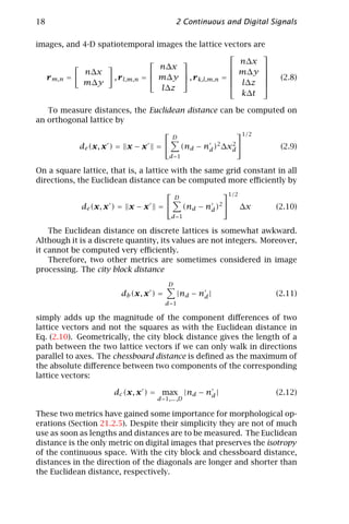
is useful to generalize the lattice vector introduced in Eq. (2.6) that rep-
resents all points of a D-dimensional digital image and can be written
as
r n = [n1 ∆x1 , n2 ∆x2 , . . . , nD ∆xD ]T (2.7)
In the preceding equation, the lattice constants ∆xd need not be equal
in all directions. For the special cases of 2-D images, 3-D volumetric](https://image.slidesharecdn.com/computervision-handbookofcomputervisionandapplicationsvolume2-signalprocessingandpatternrecognition-120205081400-phpapp02/85/Computer-vision-handbook-of-computer-vision-and-applications-volume-2-signal-processing-and-pattern-recognition-42-320.jpg)
![20 2 Continuous and Digital Signals
a b c
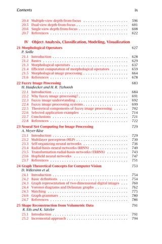
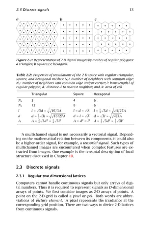
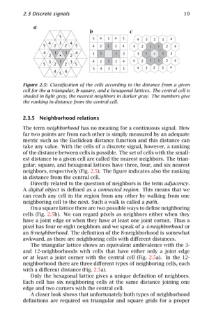
Figure 2.6: Digital objects on a triangular, b square, and c hexagonal lattice.
a and b show either two objects or one object (connected regions) depending on
the neighborhood definition.
definition of connected regions. A region or an object is called con-
nected when we can reach any pixel in the region by walking from one
neighboring pixel to the next. The black object shown in Fig. 2.6b is
one object in the 8-neighborhood, but constitutes two objects in the 4-
neighborhood. The white background, however, shows the same prop-
erty. Thus we have either two connected regions in the 8-neighborhood
crossing each other or four separated regions in the 4-neighborhood.
This inconsistency between objects and background can be overcome
if we declare the objects as 4-neighboring and the background as 8-
neighboring, or vice versa.
These complications occur also on a triangular lattice (Fig. 2.6b) but
not on a hexagonal lattice (Fig. 2.6c). The photosensors on the retina
in the human eye, however, have a more hexagonal shape, see Wandell
[1, Fig. 3.4, p. 49].
2.3.6 Errors in object position and geometry
The tessellation of space in discrete images limits the accuracy of the
estimation of the position of an object and thus all other geometri-
cal quantities such as distance, area, circumference, and orientation of
lines. It is obvious that the accuracy of the position of a single point
is only in the order of the lattice constant. The interesting question
is, however, how this error propagates into position errors for larger
objects and other relations. This question is of significant importance
because of the relatively low spatial resolution of images as compared
to other measuring instruments. Without much effort many physical
quantities such as frequency, voltage, and distance can be measured
with an accuracy better than 1 ppm, that is, 1 in 1,000,000, while im-
ages have a spatial resolution in the order of 1 in 1000 due to the limited
number of pixels. Thus only highly accurate position estimates in the](https://image.slidesharecdn.com/computervision-handbookofcomputervisionandapplicationsvolume2-signalprocessingandpatternrecognition-120205081400-phpapp02/85/Computer-vision-handbook-of-computer-vision-and-applications-volume-2-signal-processing-and-pattern-recognition-45-320.jpg)
![2.3 Discrete signals 21
order of 1/100 of the pixel size result in an accuracy of about 1 in
100,000.
The discussion of position errors in this section will be limited to or-
thogonal lattices. These lattices have the significant advantage that the
errors in the different directions can be discussed independently. Thus
the following discussion is not only valid for 2-D images but any type of
multidimensional signals and we must consider only one component.
In order to estimate the accuracy of the position estimate of a sin-
gle point it is assumed that all positions are equally probable. This
means a constant probability density function in the interval ∆x. Then
2
the variance σx introduced by the position discretization is given by
Papoulis [2, p. 106]
xn +∆x/2
2 1 (∆x)2
σx = (x − xn )2 dx = (2.13)
∆x 12
xn −∆x/2
√
Thus the standard deviation σx is about 1/ 12 ≈ 0.3 times the lattice
constant ∆x. The maximum error is, of course, 0.5∆x.
All other errors for geometrical measurements of segmented objects
can be related to this basic position error by statistical error propa-
gation. We will illustrate this with a simple example computing the
area and center of gravity of an object. For the sake of simplicity, we
start with the unrealistic assumption that any cell that contains even
the smallest fraction of the object is regarded as a cell of the object.
We further assume that this segmentation is exact, that is, the signal
itself does not contain noise and separates without errors from the
background. In this way we separate all other errors from the errors
introduced by the discrete lattice.
The area of the object is simply given as the product of the number
N of cells and the area Ac of a cell. This simple estimate is, however,
biased towards a larger area because the cells at the border of the object
are only partly covered by the object. In the mean, half of the border
cells are covered. Hence an unbiased estimate of the area is given by
A = Ac (N − 0.5Nb ) (2.14)
where Nb is the number of border cells. With this equation, the variance
of the estimate can be determined. Only the statistical error in the area
of the border cells must be considered. According to the laws of error
propagation with independent random variables, the variance of the
2
area estimate σA is given by
2
σA = 0.25A2 Nb σx
c
2
(2.15)
If we assume a compact object, for example, a square, with a length
of D pixels, it has D 2 pixels and 4D border pixels. Using σx ≈ 0.3](https://image.slidesharecdn.com/computervision-handbookofcomputervisionandapplicationsvolume2-signalprocessingandpatternrecognition-120205081400-phpapp02/85/Computer-vision-handbook-of-computer-vision-and-applications-volume-2-signal-processing-and-pattern-recognition-46-320.jpg)
![24 2 Continuous and Digital Signals
diffraction) or imperfections of the optical systems (various aberra-
tions, Volume 1, Section 4.5). This blurring of the signal is known as
the point spread function (PSF ) of the optical system and described in
the Fourier domain by the optical transfer function. The nonzero area
of the individual sensor elements of the sensor array (or the scanning
mechanism) results in a further spatial and temporal blurring of the
irradiance at the image plane.
The conversion to electrical signal U adds noise and possibly fur-
ther nonlinearities to the signal g(x, t) that is finally measured. In a
last step, the analog electrical signal is converted by an analog-to-digital
converter (ADC) into digital numbers. The basic relation between con-
tinuous and digital signals is established by the sampling theorem. It
describes the effects of spatial and temporal sampling on continuous
signals and thus also tells us how to reconstruct a continuous signal
from its samples. The discretization of the amplitudes of the signal
(quantization) is discussed in Section 2.5.
The image formation process itself thus includes two essential steps.
First, the whole image formation process blurs the signal. Second, the
continuous signal at the image plane is sampled. Although both pro-
cesses often happen together, they can be separated for an easier math-
ematical treatment.
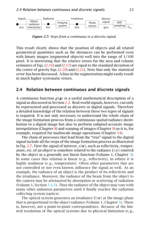
2.4.1 Image formation
If we denote the undistorted original signal projected onto the image
plane by g (x, t) then the signal g(x, t) modified by the image forma-
tion process is given by
∞
g(x, t) = g (x , t )h(x, x , t, t ) d2 x dt (2.22)
−∞
The function h is the PSF. The signal g (x, t) can be considered as the
image that would be obtained by a perfect system, that is, an optical
system whose PSF is a δ-distribution. Equation (2.22) says that the sig-
nal at the point [x, t]T in space and time is composed of the radiance of
a whole range of points [x , t ]T nearby which linearly add up weighted
with the signal h at [x , t ]T . The integral can significantly be simpli-
fied if the point spread function is the same at all points (homogeneous
system or shift-invariant system). Then the point spread function h de-
pends only on the distance of [x , t ]T to [x, t]T and the integral in
Eq. (2.22) reduces to the convolution integral
∞
g(x, t) = g (x , t )h(x − x , t − t ) d2 x dt = (g ∗ h)(x, t) (2.23)
−∞](https://image.slidesharecdn.com/computervision-handbookofcomputervisionandapplicationsvolume2-signalprocessingandpatternrecognition-120205081400-phpapp02/85/Computer-vision-handbook-of-computer-vision-and-applications-volume-2-signal-processing-and-pattern-recognition-49-320.jpg)
![2.4 Relation between continuous and discrete signals 25
For most optical systems the PSF is not strictly shift-invariant because
the degree of blurring is increasing with the distance from the optical
axis (Volume 1, Chapter 4). However, as long as the variation is con-
tinuous and does not change significantly over the width of the PSF,
the convolution integral in Eq. (2.23) still describes the image forma-
tion correctly. The PSF and the system transfer function just become
weakly dependent on x.
2.4.2 Sampling theorem
Sampling means that all information is lost except at the grid points.
Mathematically, this constitutes a multiplication of the continuous func-
tion with a function that is zero everywhere except for the grid points.
This operation can be performed by multiplying the image function
g(x) with the sum of δ distributions located at all lattice vectors r m,n
Eq. (2.7). This function is called the two-dimensional δ comb, or “nail-
board function.” Then sampling can be expressed as
m=∞ n=∞
gs (x) = g(x) δ(x − r m,n ) (2.24)
m=−∞ n=−∞
This equation is only valid as long as the elementary cell of the lattice
contains only one point. This is the case for the square and hexagonal
grids (Fig. 2.2b and c). The elementary cell of the triangular grid, how-
ever, includes two points (Fig. 2.2a). Thus for general regular lattices,
p points per elementary cell must be considered. In this case, a sum
of P δ combs must be considered, each shifted by the offsets s p of the
points of the elementary cells:
P ∞ ∞
gs (x) = g(x) δ(x − r m,n − s p ) (2.25)
p =1 m=−∞ n=−∞
It is easy to extent this equation for sampling into higher-dimensional
spaces and into the time domain:
gs (x) = g(x) δ(x − r n − s p ) (2.26)
p n
In this equation, the summation ranges have been omitted. One of the
coordinates of the D-dimensional space and thus the vector x and the
lattice vector r n
T
r n = [n1 b1 , n2 b2 , . . . , nD bD ] with nd ∈ Z (2.27)
is the time coordinate. The set of fundamental translation vectors
{b1 , b2 , . . . , bD } form a not necessarily orthogonal base spanning the
D-dimensional space.](https://image.slidesharecdn.com/computervision-handbookofcomputervisionandapplicationsvolume2-signalprocessingandpatternrecognition-120205081400-phpapp02/85/Computer-vision-handbook-of-computer-vision-and-applications-volume-2-signal-processing-and-pattern-recognition-50-320.jpg)
![26 2 Continuous and Digital Signals
The sampling theorem directly results from the Fourier transform
of Eq. (2.26). In this equation the continuous signal g(x) is multiplied
by the sum of delta distributions. According to the convolution theo-
rem of the Fourier transform (Section 3.2), this results in a convolution
of the Fourier transforms of the signal and the sum of delta combs in
Fourier space. The Fourier transform of a delta comb is again a delta
comb (see Table 3.3). As the convolution of a signal with a delta dis-
tribution simply replicates the function value at the zero point of the
delta functions, the Fourier transform of the sampled signal is simply
a sum of shifted copies of the Fourier transform of the signal:
T
ˆ
gs (k, ν) = ˆ ˆ
g(k − r v ) exp −2π ik s p (2.28)
p v
T
The phase factor exp(−2π ik s p ) results from the shift of the points in
the elementary cell by s p according to the shift theorem of the Fourier
ˆ
transform (see Table 3.2). The vectors r v
ˆ ˆ ˆ ˆ
r v = v1 b 1 + v2 b 2 + . . . + v D b D with vd ∈ Z (2.29)
are the points of the so-called reciprocal lattice. The fundamental trans-
lation vectors in the space and Fourier domain are related to each other
by
ˆ
b d b d = δ d −d (2.30)
This basically means that the fundamental translation vector in the
Fourier domain is perpendicular to all translation vectors in the spatial
domain except for the corresponding one. Furthermore the distances
are reciprocally related to each other. In 3-D space, the fundamental
translations of the reciprocial lattice can therefore be computed by
ˆ b × b d +2
b d = d +1 (2.31)
b1 (b2 × b3 )
The indices in the preceding equation are computed modulo 3, b1 (b2 ×
b3 ) is the volume of the primitive elementary cell in the spatial domain.
All these equations are familiar to solid state physicists or cristallog-
raphers [3]. Mathematicians know the lattice in the Fourier domain as
the dual base or reciprocal base of a vector space spanned by a non-
orthogonal base. For an orthogonal base, all vectors of the dual base
show into the same direction as the corresponding vectors and the mag-
ˆ
nitude is given by bd = 1/ |bd |. Then often the length of the base
vectors is denoted by ∆xd , and the length of the reciprocal vectors by
∆kd = 1/∆xd . Thus an orthonormal base is dual to itself.
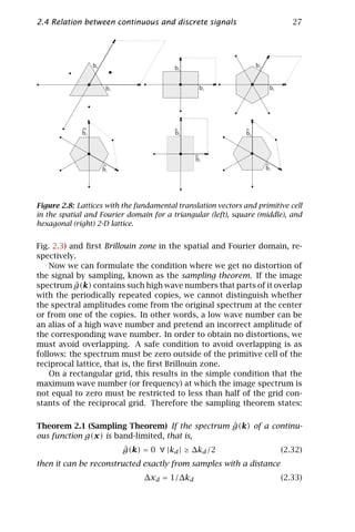
For further illustration, Fig. 2.8 shows the lattices in both domains
for a triangular, square, and hexagonal grid. The figure also includes
the primitive cell known as the Wigner-Seitz cell (Section 2.3.1 and](https://image.slidesharecdn.com/computervision-handbookofcomputervisionandapplicationsvolume2-signalprocessingandpatternrecognition-120205081400-phpapp02/85/Computer-vision-handbook-of-computer-vision-and-applications-volume-2-signal-processing-and-pattern-recognition-51-320.jpg)
![28 2 Continuous and Digital Signals
In other words, we will obtain a periodic structure correctly only if
we take at least two samples per wavelength (or period). The maximum
wave number that can be sampled without errors is called the Nyquist
or limiting wave number (or frequency). In the following, we will often
use dimensionless wave numbers (frequencies), which are scaled to the
limiting wave number (frequency). We denote this scaling with a tilde:
˜ kd ν
kd = = 2kd ∆xd and ˜
ν= = 2ν∆T (2.34)
∆kd /2 ∆ν/2
˜
In this scaling all the components of the wave number kd fall into the
interval ]−1, 1[.
2.4.3 Aliasing
If the conditions of the sampling theorem are not met, it is not only
impossible to reconstruct the original signal exactly but also distortions
are introduced into the signal. This effect is known in signal theory as
aliasing or in imaging as the Moiré effect .
The basic problem with aliasing is that the band limitation intro-
duced by the blurring of the image formation and the nonzero area of
the sensor is generally not sufficient to avoid aliasing. This is illustrated
in the following example with an “ideal” sensor.
Example 2.1: Standard sampling
An “ideal” imaging sensor will have a nonblurring optics (the PSF is the
delta distribution) and a sensor array that has a 100 % fill factor, that
is, the sensor elements show a constant sensitivity over the whole area
without gaps in-between. The PSF of such an imaging sensor is a box
function with the width ∆x of the sensor elements and the transfer
function (TF) is a sinc function (see Table 3.4):
1 1
PSF Π(x1 /∆x1 ) Π(x2 /∆x2 )
∆x1 ∆x2
(2.35)
sin(π k1 ∆x1 ) sin(π k2 ∆x2 )
TF
π k1 ∆x1 π k2 ∆x2
The sinc function has its first zero crossings when the argument is
±π . This is when kd = ±∆xd or at twice the Nyquist wave number,
see Eq. (2.34). At the Nyquist wave number the value of the transfer
√
function is still 1/ 2. Thus standard sampling is not sufficient to
avoid aliasing. The only safe way to avoid aliasing is to ensure that the
imaged objects do not contain wave numbers and frequencies beyond
the Nyquist limit.
2.4.4 Reconstruction from samples
The sampling theorem ensures the conditions under which we can re-
construct a continuous function from sampled points, but we still do](https://image.slidesharecdn.com/computervision-handbookofcomputervisionandapplicationsvolume2-signalprocessingandpatternrecognition-120205081400-phpapp02/85/Computer-vision-handbook-of-computer-vision-and-applications-volume-2-signal-processing-and-pattern-recognition-53-320.jpg)
![34 2 Continuous and Digital Signals
2.6 References
[1] Wandell, B. A., (1995). Foundations of Vision. Sunderland, MA: Sinauer
Associates.
[2] Papoulis, A., (1991). Probability, Random Variables, and Stochastic Pro-
cesses. New York: McGraw-Hill.
[3] Kittel, C., (1971). Introduction to Solid State Physics. New York: Wiley.](https://image.slidesharecdn.com/computervision-handbookofcomputervisionandapplicationsvolume2-signalprocessingandpatternrecognition-120205081400-phpapp02/85/Computer-vision-handbook-of-computer-vision-and-applications-volume-2-signal-processing-and-pattern-recognition-59-320.jpg)
![36 3 Spatial and Fourier Domain
pixels. Thus, we can compose each image of basis images m,n P where
just one pixel has a value of one while all other pixels are zero:
m,n 1 if m=m ∧n=n
Pm ,n = δm−m δn−n = (3.1)
0 otherwise
Any arbitrary image can then be composed of all basis images in Eq. (3.1)
by
M −1 N −1
G= Gm,n m,n P (3.2)
m = 0 n =0
where Gm,n denotes the gray value at the position [m, n]. The inner
product (also known as scalar product ) of two “vectors” in this space
can be defined similarly to the scalar product for vectors and is given
by
M −1 N −1
(G, H) = Gm,n Hm,n (3.3)
m =0 n=0
where the parenthesis notation (·, ·) is used for the inner product in
order to distinguish it from matrix multiplication. The basis images
m,n P form an orthonormal base for an N × M-dimensional vector space.
From Eq. (3.3), we can immediately derive the orthonormality relation
for the basis images m,n P:
M −1 N −1
m ,n
Pm,n m ,n
Pm,n = δm −m δn −n (3.4)
m =0 n=0
This says that the inner product between two base images is zero if
two different basis images are taken. The scalar product of a basis
image with itself is one. The MN basis images thus span an M × N-
dimensional vector space RN ×M over the set of real numbers.
An M × N image represents a point in the M × N vector space. If
we change the coordinate system, the image remains the same but its
coordinates change. This means that we just observe the same piece of
information from a different point of view. All these representations
are equivalent to each other and each gives a complete representation
of the image. A coordinate transformation leads us from one represen-
tation to the other and back again. An important property of such a
transform is that the length or (magnitude) of a vector
1/2
G 2 = (G, G) (3.5)
is not changed and that orthogonal vectors remain orthogonal. Both
requirements are met if the coordinate transform preserves the inner](https://image.slidesharecdn.com/computervision-handbookofcomputervisionandapplicationsvolume2-signalprocessingandpatternrecognition-120205081400-phpapp02/85/Computer-vision-handbook-of-computer-vision-and-applications-volume-2-signal-processing-and-pattern-recognition-61-320.jpg)
![3.1 Vector spaces and unitary transforms 37
product. A transform with this property is known as a unitary trans-
form.
Physicists will be reminded of the theoretical foundations of quan-
tum mechanics, which are formulated in an inner product vector space
of infinite dimension, the Hilbert space.
3.1.2 Basic properties of unitary transforms
The two most important properties of a unitary transform are [1]:
Theorem 3.1 (Unitary transform) Let V be a finite-dimensional inner
product vector space. Let U be a one-one linear transformation of V
onto itself. Then
1. U preserves the inner product, that is, (G, H) = (UG, UH), ∀G, H ∈
V.
T T
2. The inverse of U, U −1 , is the adjoin U ∗ of U : UU ∗ = I.
Rotation in R2 or R3 is an example of a transform where the preser-
vation of the length of vectors is obvious.
The product of two unitary transforms U 1 U 2 is unitary. Because
the identity operator I is unitary, as is the inverse of a unitary operator,
the set of all unitary transforms on an inner product space is a group
under the operation of composition. In practice, this means that we
can compose/decompose complex unitary transforms of/into simpler
or elementary transforms.
3.1.3 Significance of the Fourier transform (FT)
A number of unitary transforms have gained importance for digital
signal processing including the cosine, sine, Hartley, slant, Haar, and
Walsh transforms [2, 3, 4]. But none of these transforms matches in
importance with the Fourier transform.
The uniqueness of the Fourier transform is related to a property
expressed by the shift theorem. If a signal is shifted in space, its Fourier
transform does not change in amplitude but only in phase, that is, it
is multiplied with a complex phase factor. Mathematically this means
that all base functions of the Fourier transform are eigenvectors of the
shift operator S(s):
S(s) exp(−2π ikx) = exp(−2π iks) exp(−2π ikx) (3.6)
The phase factor exp(−2π iks) is the eigenvalue and the complex ex-
ponentials exp(−2π ikx) are the base functions of the Fourier trans-
form spanning the infinite-dimensional vector space of the square in-
tegrable complex-valued functions over R. For all other transforms,
various base functions are mixed with each other if one base function](https://image.slidesharecdn.com/computervision-handbookofcomputervisionandapplicationsvolume2-signalprocessingandpatternrecognition-120205081400-phpapp02/85/Computer-vision-handbook-of-computer-vision-and-applications-volume-2-signal-processing-and-pattern-recognition-62-320.jpg)
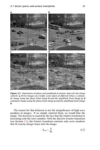
![40 3 Spatial and Fourier Domain
a
k2 b
k2
kd ϕ
kdlnk
k1
k1
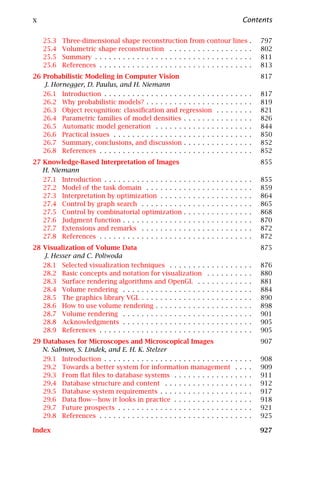
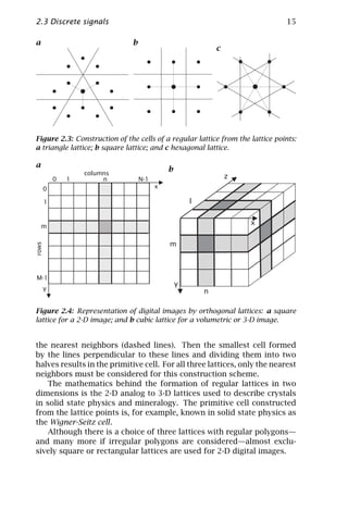
Figure 3.2: Tessellation of the 2-D Fourier domain into: a Cartesian; and b
logarithmic-polar lattices.
T
where d = [d1 , . . . , dD ] is the size of the D-dimensional signal. There-
fore the absolute wave number resolution ∆k = 1/∆x is constant,
equivalent to a Cartesian tessellation of the Fourier space (Fig. 3.2a).
Thus the smallest wave number (v = 1) has a wavelength of the size of
the image, the next coarse wave number a wavelength of half the size
of the image. This is a very low resolution for large wavelengths. The
smaller the wavelength, the better the resolution.
This ever increasing relative resolution is not natural. We can, for
example, easily see the difference of 10 cm in 1 m, but not in 1 km. It
is more natural to think of relative resolutions, because we are better
able to distinguish relative distance differences than absolute ones. If
we apply this concept to the Fourier domain, it seems to be more natural
to tessellate the Fourier domain in intervals increasing with the wave
number, a log-polar coordinate system, as illustrated in Fig. 3.2b. Such a
lattice partitions the space into angular and lnk intervals. Thus, the cell
area is proportional to k2 . In order to preserve the norm, or—physically
spoken—the energy, of the signal in this representation, the increase
in the area of the cells proportional to k2 must be considered:
∞ ∞
2
ˆ
|g(k)| dk1 dk2 = k2 |g(k)|2 d ln k dϕ
ˆ (3.8)
−∞ −∞
Thus, the power spectrum |g(k)|2 in the log-polar representation is
ˆ
multiplied by k2 and falls off much less steep than in the Cartesian
representation. The representation in a log-polar coordinate system al-
lows a much better evaluation of the directions of the spatial structures](https://image.slidesharecdn.com/computervision-handbookofcomputervisionandapplicationsvolume2-signalprocessingandpatternrecognition-120205081400-phpapp02/85/Computer-vision-handbook-of-computer-vision-and-applications-volume-2-signal-processing-and-pattern-recognition-65-320.jpg)
![3.2 Continuous Fourier transform (FT) 41
and of the smaller scales. Moreover a change in scale or orientation just
causes a shift of the signal in the log-polar representation. Therefore
it has gained importance in representation object for shape analysis
(Volume 3, Chapter 8).
3.2 Continuous Fourier transform (FT)
In this section, we give a brief survey of the continuous Fourier trans-
form and we point out the properties that are most important for signal
processing. Extensive and excellent reviews of the Fourier transform
are given by Bracewell [5], Poularikas [4, Chapter 2] or Madisetti and
Williams [6, Chapter 1]
3.2.1 One-dimensional FT
Definition 3.1 (1-D FT) If g(x) : R C is a square integrable function,
that is,
∞
g(x) dx < ∞ (3.9)
−∞
ˆ
then the Fourier transform of g(x), g(k) is given by
∞
ˆ
g(k) = g(x) exp (−2π ikx) dx (3.10)
−∞
The Fourier transform maps the vector space of absolutely integrable
ˆ
functions onto itself. The inverse Fourier transform of g(k) results in
the original function g(x):
∞
g(x) = ˆ
g(k) exp (2π ikx) dk (3.11)
−∞
It is convenient to use an operator notation for the Fourier trans-
form. With this notation, the Fourier transform and its inverse are
simply written as
ˆ
g(k) = F g(x) and g(x) = F −1 g(k)
ˆ (3.12)
A function and its transform, a Fourier transform pair is simply de-
⇒ ˆ
noted by g(x) ⇐ g(k).
In Eqs. (3.10) and (3.11) a definition of the wave number without the
factor 2π is used, k = 1/λ, in contrast to the notation often used in](https://image.slidesharecdn.com/computervision-handbookofcomputervisionandapplicationsvolume2-signalprocessingandpatternrecognition-120205081400-phpapp02/85/Computer-vision-handbook-of-computer-vision-and-applications-volume-2-signal-processing-and-pattern-recognition-66-320.jpg)
![42 3 Spatial and Fourier Domain
Table 3.1: Comparison of the continuous Fourier transform (FT), the Fourier
series (FS), the infinite discrete Fourier transform (IDFT), and the discrete Fourier
transform (DFT) in one dimension
Type Forward transform Backward transform
∞ ∞
FT: R ⇐ R
⇒ g(x) exp (−2π ikx) dx ˆ
g(k) exp (2π ikx) dk
−∞ −∞
∆x ∞
FS: 1 vx vx
g(x) exp −2π i dx ˆ
gv exp 2π i
[0, ∆x] ⇐ Z
⇒ ∆x ∆x v =−∞
∆x
0
1/∆x
∞
IDFT:
gn exp (−2π in∆xk) ∆x ˆ
g(k) exp (2π in∆xk) dk
Z ⇐ [0, 1/∆x]
⇒ n=−∞
0
N −1 N −1
DFT: 1 vn vn
gn exp −2π i ˆ
gv exp 2π i
N N ⇐ NN
⇒ N n=0 N N
v =0
physics with k = 2π /λ. For signal processing, the first notion is more
useful, because k directly gives the number of periods per unit length.
With the notation that includes the factor 2π in the wave number,
two forms of the Fourier transform are common, the asymmetric form
∞
ˆ
g(k ) = g(x) exp(−ik x) dx
−∞
∞ (3.13)
1
g(x) = ˆ
g(k) exp(ik x) dk
2π
−∞
and the symmetric form
∞
1
g(k ) = √
ˆ g(x) exp(−ik x) dx
2π
−∞
∞ (3.14)
1
g(x) = √ ˆ
g(k ) exp(ik x) dk
2π
−∞
As the definition of the Fourier transform takes the simplest form
in Eqs. (3.10) and (3.11), most other relations and equations also be-
come simpler than with the definitions in Eqs. (3.13) and (3.14). In
addition, the relation of the continuous Fourier transform with the dis-
crete Fourier transform (Section 3.3) and the Fourier series (Table 3.1)
becomes more straightforward.
Because all three versions of the Fourier transform are in common
use, it is likely to get wrong factors in Fourier transform pairs. The rules](https://image.slidesharecdn.com/computervision-handbookofcomputervisionandapplicationsvolume2-signalprocessingandpatternrecognition-120205081400-phpapp02/85/Computer-vision-handbook-of-computer-vision-and-applications-volume-2-signal-processing-and-pattern-recognition-67-320.jpg)
![3.2 Continuous Fourier transform (FT) 43
for conversion of Fourier transform pairs between the three versions
can directly be inferred from the definitions and are summarized here:
k without 2π , Eq. (3.10) g(x) ⇐⇒ ˆ
g(k)
k with 2π , Eq. (3.13) g(x) ⇐⇒ ˆ
g(k /2π ) (3.15)
k with 2π , Eq. (3.14) g(x/ (2π )) ⇐⇒ ˆ
g(k / (2π ))
3.2.2 Multidimensional FT
The Fourier transform can easily be extended to multidimensional sig-
nals.
Definition 3.2 (Multidimensional FT) If g(x) : RD C is a square in-
tegrable function, that is,
∞
g(x) dDx < ∞ (3.16)
−∞
ˆ
then the Fourier transform of g(x), g(k) is given by
∞
T
ˆ
g(k) = g(x) exp −2π ik x dDx (3.17)
−∞
and the inverse Fourier transform by
∞
T
g(x) = g(k) exp 2π ik x dDk
ˆ (3.18)
−∞
The scalar product in the exponent of the kernel x T k makes the
kernel of the Fourier transform separable, that is, it can be written as
D
T
exp −2π ik x = exp(−ikd xd ) (3.19)
d =1
3.2.3 Basic properties
For reference, the basic properties of the Fourier transform are summa-
rized in Table 3.2. An excellent review of the Fourier transform and its
applications are given by [5]. Here we will point out some of the prop-
erties of the FT that are most significant for multidimensional signal
processing.](https://image.slidesharecdn.com/computervision-handbookofcomputervisionandapplicationsvolume2-signalprocessingandpatternrecognition-120205081400-phpapp02/85/Computer-vision-handbook-of-computer-vision-and-applications-volume-2-signal-processing-and-pattern-recognition-68-320.jpg)
![46 3 Spatial and Fourier Domain
In signal processing, the function h(x) is normally zero except for a
small area around zero and is often denoted as the convolution mask.
Thus, the convolution with h(x) results in a new function g (x) whose
values are a kind of weighted average of g(x) in a small neighborhood
around x. It changes the signal in a defined way, that is, makes it
smoother etc. Therefore it is also called a filter operation. The convo-
lution theorem states:
ˆ
Theorem 3.2 (Convolution) If g(x) has the Fourier transform g(k) and
ˆ
h(x) has the Fourier transform h(k) and if the convolution integral
ˆ ˆ
(Eq. (3.25)) exists, then it has the Fourier transform h(k)g(k).
Thus, convolution of two functions means multiplication of their
transforms. Likewise convolution of two functions in the Fourier do-
main means multiplication in the space domain. The simplicity of con-
volution in the Fourier space stems from the fact that the base func-
T
tions of the Fourier domain, the complex exponentials exp 2π ik x ,
are joint eigenfunctions of all convolution operators. This means that
these functions are not changed by a convolution operator except for
the multiplication by a factor.
From the convolution theorem, the following properties are imme-
diately evident. Convolution is
commutative h ∗ g = g ∗ h,
associative h1 ∗ (h2 ∗ g) = (h1 ∗ h2 ) ∗ g, (3.26)
distributive over addition (h1 + h2 ) ∗ g = h1 ∗ g + h2 ∗ g
In order to grasp the importance of these properties of convolu-
tion, we note that two operations that do not look so at first glance,
are also convolution operations: the shift operation and all derivative
operators. This can immediately be seen from the shift and derivative
theorems (Table 3.2 and [5, Chapters 5 and 6]).
In both cases the Fourier transform is just multiplied by a complex
factor. The convolution mask for a shift operation S is a shifted δ
distribution:
S(s)g(x) = δ(x − s) ∗ g(x) (3.27)
The transform of the first derivative operator in x1 direction is
2π ik1 . The corresponding inverse Fourier transform of 2π ik1 , that
is, the convolution mask, is no longer an ordinary function (2π ik1 is
not absolutely integrable) but the derivative of the δ distribution:
dδ(x) d exp(−π x 2 /a2 )
2π ik1 ⇐⇒ δ (x) = = lim (3.28)
dx a→0 dx a](https://image.slidesharecdn.com/computervision-handbookofcomputervisionandapplicationsvolume2-signalprocessingandpatternrecognition-120205081400-phpapp02/85/Computer-vision-handbook-of-computer-vision-and-applications-volume-2-signal-processing-and-pattern-recognition-71-320.jpg)
![3.2 Continuous Fourier transform (FT) 47
Of course, the derivation of the δ distribution exists—as all properties
of distributions—only in the sense as a limit of a sequence of functions
as shown in the preceding equation.
With the knowledge of derivative and shift operators being convo-
lution operators, we can use the properties summarized in Eq. (3.26) to
draw some important conclusions. As any convolution operator com-
mutes with the shift operator, convolution is a shiftinvariant operation.
Furthermore, we can first differentiate a signal and then perform a con-
volution operation or vice versa and obtain the same result.
The properties in Eq. (3.26) are essential for an effective computa-
tion of convolution operations as discussed in Section 5.6. As we al-
ready discussed qualitatively in Section 3.1.3, the convolution operation
is a linear shiftinvariant operator. As the base functions of the Fourier
domain are the common eigenvectors of all linear and shiftinvariant op-
erators, the convolution simplifies to a complex multiplication of the
transforms.
Central-limit theorem. The central-limit theorem is mostly known for
its importance in the theory of probability [7]. It also plays, however, an
important role for signal processing as it is a rigorous statement of the
tendency that cascaded convolution tends to approach Gaussian form
(∝ exp(−ax 2 )). Because the Fourier transform of the Gaussian is also
a Gaussian (Table 3.3), this means that both the Fourier transform (the
transfer function) and the mask of a convolution approach Gaussian
shape. Thus the central-limit theorem is central to the unique role of
the Gaussian function for signal processing. The sufficient conditions
under which the central limit theorem is valid can be formulated in
different ways. We use here the conditions from [7] and express the
theorem with respect to convolution.
Theorem 3.3 (Central-limit theorem) Given N functions hn (x) with
∞ ∞
zero mean −∞ hn (x) dx and the variance σn = −∞ x 2 hn (x) dx with
2
N
z = x/σ , σ 2 = n=1 σn then
2
h = lim h1 ∗ h2 ∗ . . . ∗ hN ∝ exp(−z2 /2) (3.29)
N →∞
provided that
N
2
lim σn → ∞ (3.30)
N →∞
n=1
and there exists a number α > 2 and a finite constant c such that
∞
x α hn (x) dx < c < ∞ ∀n (3.31)
−∞](https://image.slidesharecdn.com/computervision-handbookofcomputervisionandapplicationsvolume2-signalprocessingandpatternrecognition-120205081400-phpapp02/85/Computer-vision-handbook-of-computer-vision-and-applications-volume-2-signal-processing-and-pattern-recognition-72-320.jpg)
![50 3 Spatial and Fourier Domain
Table 3.4: Important transform pairs for the continuous Fourier transform; 2-
D and 3-D functions are marked by † and ‡, respectively; for pictorial of Fourier
transform pairs, see [4, 5]
Space domain Fourier domain
δ(x) 1
Derivative of delta, δ (x) 2π ik
1
cos(2π k0 x) II(k/k0 ) = (δ(k − k0 ) + δ(k + k0 ))
2
i
sin(2π k0 x) II(k/k0 ) = (δ(k − k0 ) − δ(k + k0 ))
2
1 |x | < 1/2 sin(π k)
Box Π(x) = sinc(k) =
0 |x | ≥ 1/2 πk
1 − |x | |x | < 1 sin2 (π k)
Triangle, Λ(x) = sinc2 (k) =
0 |x | ≥ 1 π 2 k2
|x | J1 (2π k )
Disk† , Π Bessel,
2 k
|x | sin(2π k) − 2π k cos(2π k)
Ball‡ , Π
2 2π 2 k3
1/2 k J1 (2π x)
Half circle, 1 − k2 Π 2 Bessel,
2x
2
exp(−|x |) Lorentzian,
1 + (2π k)2
1 x≥0 −i
sgn(x) =
−1 x < 0 πk
1 x ≥ 0 1 i
Unit step, U(x) = δ(k) −
0 x < 0 2 2π k
1
Relaxation, exp(−|x |)U (x)
1 + 2π ik
exp(π x) − exp(−π x) −2i
tanh(π x) = cosech,
exp(π x) + exp(−π x) exp(2π k) − exp(−2π k)
Table 3.4 summarizes the most important other Fourier transform
pairs. It includes a number of special functions that are often used in
signal processing. The table contains various impulse forms, among
others the Gaussian (in Table 3.3), the box function Π, the triangle func-
tion Λ, and the Lorentzian function. In the table important transition
functions such as the Heaviside unit step function, U , the sign function,
sgn, and the hyperbolic tangent , tanh, function are also defined.](https://image.slidesharecdn.com/computervision-handbookofcomputervisionandapplicationsvolume2-signalprocessingandpatternrecognition-120205081400-phpapp02/85/Computer-vision-handbook-of-computer-vision-and-applications-volume-2-signal-processing-and-pattern-recognition-75-320.jpg)
![3.3 The discrete Fourier transform (DFT) 51
3.3 The discrete Fourier transform (DFT)
3.3.1 One-dimensional DFT
Definition 3.3 (1-D DFT) If g is an N-dimensional complex-valued vec-
tor,
g = [g0 , g1 , . . . , gN −1 ]T (3.35)
ˆ
then the discrete Fourier transform of g, g is defined as
N −1
1 2π inv
gv = √
ˆ gn exp − , 0≤v <N (3.36)
N n= 0 N
The DFT maps the vector space of N-dimensional complex-valued
vectors onto itself. The index v denotes how often the wavelength
of the corresponding discrete exponential exp(−2π inv/N) with the
ˆ
amplitude gv fits into the interval [0, N].
The back transformation is given by
N −1
1 2π inv
gn = √ ˆ
gv exp , 0≤n<N (3.37)
N v =0 N
We can consider the DFT as the inner product of the vector g with a set
of M orthonormal basis vectors, the kernel of the DFT:
1 v 2v (N −1)v T 2π i
bv = √ 1, WN , WN , . . . , WN with WN = exp (3.38)
N N
Using the base vectors bv , the DFT reduces to
∗T
b0
∗T
b1
F =
∗T
ˆ
gv = b g ˆ
or g = Fg with (3.39)
...
∗T
b N −1
ˆ
This means that the coefficient gv in the Fourier space is obtained by
projecting the vector g onto the basis vector bv . The N basis vectors
bv form an orthonormal base of the vector space:
∗T 1 if v =v
b v b v = δ v −v = (3.40)
0 otherwise
The real and imaginary parts of the basis vectors are sampled sine
and cosine functions of different wavelengths (Fig. 3.3) with a charac-
teristic periodicity:
2π in + pN 2π in
exp = exp , ∀p ∈ Z (3.41)
N N](https://image.slidesharecdn.com/computervision-handbookofcomputervisionandapplicationsvolume2-signalprocessingandpatternrecognition-120205081400-phpapp02/85/Computer-vision-handbook-of-computer-vision-and-applications-volume-2-signal-processing-and-pattern-recognition-76-320.jpg)
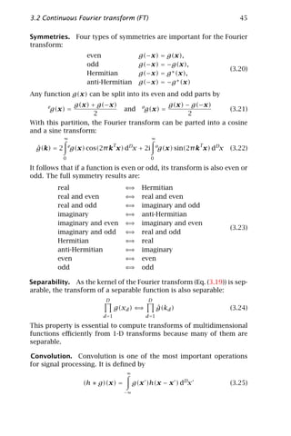
![52 3 Spatial and Fourier Domain
2
0
1
3 4 5
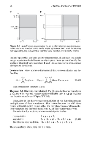
Figure 3.3: The first six basis functions (cosine part) of the DFT for N = 32 in a
cyclic representation on the unit circle.
The basis vector b0 is a constant real vector.
With this relation and Eqs. (3.36) and (3.37) the DFT and the in-
ˆ
verse DFT extend the vectors g and g, respectively, periodically over
the whole space:
Fourier domain ˆ ˆ
gv +pN = gv , ∀p ∈ Z
(3.42)
space domain gn+pN = gn ∀p ∈ Z
This periodicity of the DFT gives rise to an interesting geometric inter-
pretation. According to Eq. (3.42) the border points gM −1 and gM = g0
are neighboring points. Thus it is natural to draw the points of the
vector not on a finite line but on a unit circle, or Fourier ring (Fig. 3.3).
With the double periodicity of the DFT, it does not matter which
range of N indices we chose. The most natural choice of wave numbers
is v ∈ [−N/2, N/2 − 1], N even. With this index range the 1-D DFT and
its inverse are defined as
N −1 N/2−1
1 1
gv = √
ˆ gn WN nv ⇐ gn = √
−
⇒ ˆ nv
gv WN (3.43)
N n=0 N v =−N/2
Then the wave numbers are restricted to values that meet the sam-
pling theorem (Section 2.4.2), that is, are sampled at least two times](https://image.slidesharecdn.com/computervision-handbookofcomputervisionandapplicationsvolume2-signalprocessingandpatternrecognition-120205081400-phpapp02/85/Computer-vision-handbook-of-computer-vision-and-applications-volume-2-signal-processing-and-pattern-recognition-77-320.jpg)
![54 3 Spatial and Fourier Domain
3.3.3 Basic properties
The theorems of the 2-D DFT are summarized in Table 3.5. They are
very similar to the corresponding theorems of the continuous Fourier
transform, which are listed in Table 3.2 for a D-dimensional FT. As in
Section 3.2.3, we discuss some properties that are of importance for
signal processing in more detail.
Symmetry. The DFT shows the same symmetries as the FT (Eq. (3.20)).
In the definition for even and odd functions g(−x) = ±g(x) only the
continuous functions must be replaced by the corresponding vectors
g−n = ±gn or matrices G−m,−n = ±Gm,n . Note that because of the
periodicity of the DFT, these symmetry relations can also be written as
G−m,−n = ±Gm,n ≡ GM −m,N −n = ±Gm,n (3.48)
for even (+ sign) and odd (− sign) functions. This is equivalent to shift-
ing the symmetry center from the origin to the point [M/2, N/2]T .
The study of symmetries is important for practical purposes. Care-
ful consideration of symmetry allows storage space to be saved and
algorithms to speed up. Such a case is real-valued images. Real-valued
images can be stored in half of the space as complex-valued images.
From the symmetry relations Eq. (3.23) we can conclude that real-valued
functions exhibit a Hermitian DFT:
∗
Gmn = Gmn ⇐⇒ ˆ ˆ∗
GM −u,N −v = Guv (3.49)
The complex-valued DFT of real-valued matrices is, therefore, com-
pletely determined by the values in one half-space. The other half-space
is obtained by mirroring at the symmetry center (M/2, N/2). Conse-
quently, we need the same amount of storage space for the DFT of a
real image as for the image itself, as only half of the complex spectrum
needs to be stored.
In two and higher dimensions, matters are slightly more complex.
The spectrum of a real-valued image is determined completely by the
values in one half-space, but there are many ways to select the half-
space. This means that all except for one component of the wave num-
ber can be negative, but that we cannot distinguish between k and −k,
that is, between wave numbers that differ only in sign. Therefore we
can again represent the Fourier transform of real-valued images in a
half-space where only one component of the wave number includes
negative values. For proper representation of the spectra with zero
values of this component in the middle of the image, it is necessary to
interchange the upper (positive) and lower (negative) parts of the image
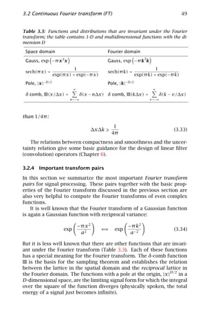
as illustrated in Fig. 3.4.
For real-valued image sequences, again we need only a half-space to
represent the spectrum. Physically, it makes the most sense to choose](https://image.slidesharecdn.com/computervision-handbookofcomputervisionandapplicationsvolume2-signalprocessingandpatternrecognition-120205081400-phpapp02/85/Computer-vision-handbook-of-computer-vision-and-applications-volume-2-signal-processing-and-pattern-recognition-79-320.jpg)
![3.3 The discrete Fourier transform (DFT) 55
Table 3.5: Summary of the properties of the 2-D DFT; G and H are complex-
ˆ ˆ
valued M × N matrices, G and H their Fourier transforms, and a and b complex-
valued constants; for proofs see Poularikas [4], Cooley and Tukey [8]
Property Space domain Wave number domain
M −1 N −1
1 √
Mean Gmn ˆ
G0,0 / MN
MN m=0 n=0
Linearity aG + bH ˆ ˆ
aG + b H
Shifting Gm−m ,n−n − ˆ
WMm u WN n v Guv
−
Modulation WM m WN n Gm,n
u v ˆ
Gu−u ,v −v
(Gm+1,n − Gm−1,n )/2 ˆ
i sin(2π u/M)Guv
Finite differences
(Gm,n+1 − Gm,n−1 )/2 ˆ
i sin(2π v/N)Guv
Spatial GP m,Qn ˆ
Guv /( P Q)
stretching
Frequency Gm,n /( P Q) ˆ
GP u,Qv
stretching
P −1Q−1
1 ˆ
Spatial sampling Gm/P ,n/Q Gu+pM/P ,v +qN/Q
P Q p=0 q=0
P −1Q−1
1 ˆ
Frequency Gm+pM/P ,n+qN/Q Gpu,qv
P Q p=0 q=0
sampling
M −1 N −1
√
Convolution Hm n Gm−m ,n−n ˆ ˆ
MN Huv Guv
m =0n =0
M −1 N −1
√
Multiplication MNGmn Hmn Hu v Gu−u ,v −v
u =0v =0
M −1 N −1
√
Spatial Hm n Gm+m ,n+n ˆ ˆ∗
N Huv Guv
correlation m =0n =0
M −1 N −1 M −1N −1
Inner product Gmn Hmn
∗ ˆ ˆ∗
Guv Huv
m=0 n=0 u=0 v =0
M −1 N −1 M −1N −1
Norm |Gmn |2 ˆ
|Guv |2
m=0 n=0 u=0 v =0](https://image.slidesharecdn.com/computervision-handbookofcomputervisionandapplicationsvolume2-signalprocessingandpatternrecognition-120205081400-phpapp02/85/Computer-vision-handbook-of-computer-vision-and-applications-volume-2-signal-processing-and-pattern-recognition-80-320.jpg)
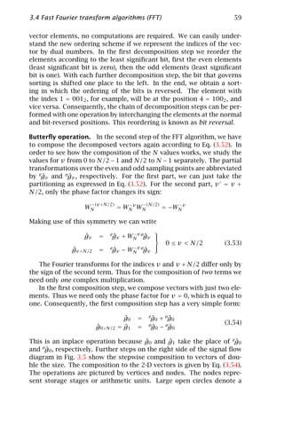
![3.4 Fast Fourier transform algorithms (FFT) 57
3.4 Fast Fourier transform algorithms (FFT)
Without an effective algorithm to calculate the discrete Fourier trans-
form, it would not be possible to apply the FT to images and other
higher-dimensional signals. Computed directly after Eq. (3.45), the FT
is prohibitively expensive. Not counting the calculations of the cosine
and sine functions in the kernel, which can be precalculated and stored
in a lookup table, the FT of an N × N image needs in total N 4 complex
multiplications and N 2 (N 2 − 1) complex additions. Thus it is an op-
eration of O(N 4 ) and the urgent need arises to minimize the number
of computations by finding a suitable fast algorithm. Indeed, the fast
Fourier transform (FFT) algorithm first published by Cooley and Tukey
[8] is the classical example of a fast algorithm. The strategies discussed
in the following for various types of FFTs are also helpful for other fast
algorithms.
3.4.1 One-dimensional FFT algorithms
Divide-and-conquer strategy. First we consider fast algorithms for
the 1-D DFT, commonly abbreviated as FFT algorithms for fast Fourier
transform. We assume that the dimension of the vector is a power
of two, N = 2l . Because the direct solution according to Eq. (3.36) is
O(N 2 ), it seems useful to use the divide-and-conquer strategy. If we
can split the transformation into two parts with vectors the size of N/2,
we reduce the number of operations from N 2 to 2(N/2)2 = N 2 /2. This
procedure can be applied recursively ld N times, until we obtain a vector
of size 1, whose DFT is trivial because nothing at all has to be done. Of
course, this procedure works only if the partitioning is possible and the
number of additional operations to put the split transforms together
is not of a higher order than O(N).
The result of the recursive partitioning is puzzling. We do not have
to perform a DFT at all. The whole algorithm to compute the DFT has
been shifted over to the recursive composition stages. If these com-
positions are of the order O(N), the computation of the DFT totals to
O(N ld N) because ld N compositions have to be performed. In com-
parison to the direct solution of the order O(N 2 ), this is a tremendous
saving in the number of operations. For N = 210 (1024), the number is
reduced by a factor of about 100. In the following we detail the radix-2
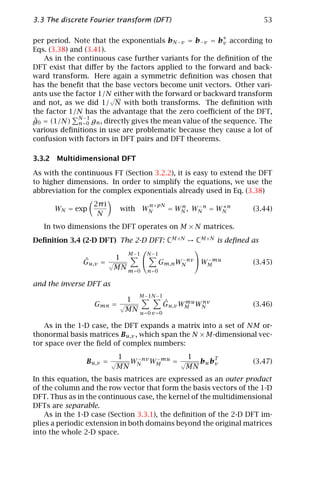
decimation in time FFT algorithm. The name of this algorithm comes
from the partition into two parts in the spatial (time) domain. We will
first show that the decomposition is possible, that it implies a reorder-
ing of the elements of the vector (bitreversal), and then discuss the
central operation of the composition stage, the butterfly operation.](https://image.slidesharecdn.com/computervision-handbookofcomputervisionandapplicationsvolume2-signalprocessingandpatternrecognition-120205081400-phpapp02/85/Computer-vision-handbook-of-computer-vision-and-applications-volume-2-signal-processing-and-pattern-recognition-82-320.jpg)
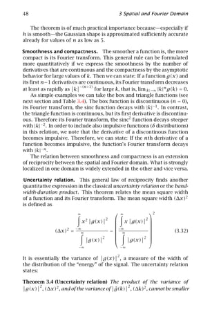
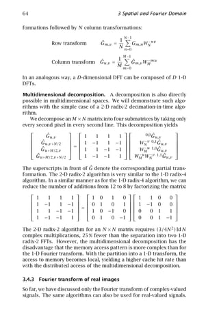
![60 3 Spatial and Fourier Domain
g0 g0 g0 ^
g0
000 000 000 000
g1 g2 g4
1
001 010 100
g2 g4 g2
1
010 100 010
g3 g6 g6
1
011 110 110
g4 g1 g1 ^
g4
1
100 001 001 100
g5 g3 g5
1
101 011 101
g6 g5 g3 1
110 101 011
g7 g7 g7
1
111 111 111
1 2 3
Decomposition = bit reversal Composition stages
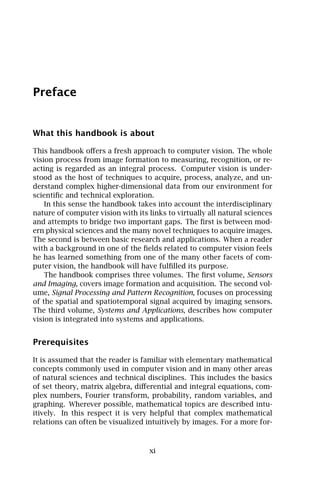
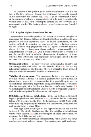
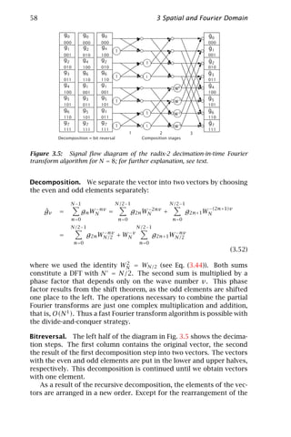
Figure 3.6: ˆ ˆ
Signal flow path for the calculation of g0 and g4 with the
decimation-in-time FFT algorithm for an 8-dimensional vector.
multiplication by the factor written into the circle. Small open circles
are adder stages. The figures from all incoming vertices are added up;
those with an open arrowhead are subtracted.
The elementary operation of the FFT algorithm involves only two
nodes. The lower node is multiplied with a phase factor. The sum and
difference of the two values are then transferred to the upper and lower
node, respectively. Because of the crossover of the signal paths, this
operation is denoted as a butterfly operation.
We gain further insight into the FFT algorithm if we trace back the
calculation of a single element. Figure 3.6 shows the signal paths for
ˆ ˆ
g0 and g4 . For each level we go back the number of knots contributing
to the calculation doubles. In the last stage all elements are involved.
ˆ ˆ
The signal path for g0 and g4 are identical but for the last stage, thus
nicely demonstrating the efficiency of the FFT algorithm.
ˆ
All phase factors in the signal path for g0 are one. As expected from
ˆ
Eq. (3.36), g0 contains the sum of all the elements of the vector g,
ˆ
g0 = [(g0 + g4 ) + (g2 + g6 )] + [(g1 + g5 ) + (g3 + g7 )]
ˆ
while for g4 the addition is replaced by a subtraction:
ˆ
g4 = [(g0 + g4 ) + (g2 + g6 )] − [(g1 + g5 ) + (g3 + g7 )]
Computational costs. After this detailed discussion of the algorithm,
we can now estimate the necessary number of operations. At each stage
of the composition, N/2 complex multiplications and N complex addi-
tions are carried out. In total we need N/2 ldN complex multiplications
and N ldN complex additions. A more extensive analysis shows that we](https://image.slidesharecdn.com/computervision-handbookofcomputervisionandapplicationsvolume2-signalprocessingandpatternrecognition-120205081400-phpapp02/85/Computer-vision-handbook-of-computer-vision-and-applications-volume-2-signal-processing-and-pattern-recognition-85-320.jpg)
![3.4 Fast Fourier transform algorithms (FFT) 61
can save even more multiplications. In the first two composition steps
only trivial multiplications by 1 or i occur (compare Fig. 3.6). For fur-
ther steps the number of trivial multiplications decreases by a factor
of two. If our algorithm could avoid all the trivial multiplications, the
number of multiplications would be reduced to (N/2)(ld N − 3).
Using the FFT algorithm, the discrete Fourier transform can no longer
be regarded as a computationally expensive operation, as only a few op-
erations are necessary per element of the vector. For a vector with 512
elements, only 3 complex multiplications and 8 complex additions, cor-
responding to 12 real multiplications and 24 real additions, need to be
computed per pixel.
Radix-4 FFT. The radix-2 algorithm discussed in the preceding is only
one of the many divide-and-conquer strategies to speed up Fourier
transform. It belongs to the class of Cooley-Tukey algorithms [9]. In-
stead of parting the vector into two pieces, we could have chosen any
other partition, say P Q-dimensional vectors, if N = P Q.
An often-used partition is the radix-4 FFT algorithm decomposing
the vector into four components:
N/4−1 N/4−1
ˆ
gv = g4n WN 4nv + WN v
− −
g4n+1 WN 4nv
−
n=0 n=0
N/4−1 N/4−1
+ WN 2v
−
g4n+2 WN 4nv + WN 3v
− −
g4n+3 WN 4nv
−
n=0 n =0
For simpler equations, we will use similar abbreviations as for the radix-
2 algorithm and denote the partial transformations by 0g, · · · ,3 g. Mak-
ˆ ˆ
v
ing use of the symmetry of WN , the transformations into quarters of
each of the vectors is given by
ˆ
gv = 0g
ˆv + WN v 1gv + WN 2v 2gv + WN 3v 3gv
−
ˆ −
ˆ −
ˆ
ˆ
gv +N/4 = 0g
ˆv − iWN v 1gv − WN 2v 2gu + iWN 3v 3gv
−
ˆ −
ˆ −
ˆ
ˆ
gv +N/2 = 0g
ˆv − WN v 1gv + WN 2v 2gv − WN 3v 3gv
−
ˆ −
ˆ −
ˆ
ˆ
gv +3N/4 = 0g
ˆv + iWN v 1gv − WN 2v 2gv − iWN 3v 3gv
−
ˆ −
ˆ −
ˆ
or, in matrix notation,
ˆ
gv 1 1 1 1 0gˆv
−v 1
gv +N/4
ˆ = 1 −i −1 i WN gv ˆ
g −2v 2
ˆv +N/2 1 −1 1 −1 WN ˆ
gv
ˆ
gv +3N/4 1 i −1 −i WN 3v 3gv
−
ˆ
To compose 4-tuple elements of the vector, 12 complex additions and
3 complex multiplications are needed. We can reduce the number of](https://image.slidesharecdn.com/computervision-handbookofcomputervisionandapplicationsvolume2-signalprocessingandpatternrecognition-120205081400-phpapp02/85/Computer-vision-handbook-of-computer-vision-and-applications-volume-2-signal-processing-and-pattern-recognition-86-320.jpg)

![3.4 Fast Fourier transform algorithms (FFT) 65
Then they are less efficient, however, as the Fourier transform of a
real-valued signal is Hermitian (Section 3.2.3) and thus only half of the
Fourier coefficients are independent. This corresponds to the fact that
also half of the signal, namely the imaginary part, is zero.
It is obvious that another factor two in computational speed can be
gained for the DFT of real data. Three common strategies [2] that are
used to map real vectors onto complex vectors are discussed in what
follows.
Mapping of two real vectors onto one complex vector. The easiest
way to do so is to compute two real 1-D sequences at once. This concept
can easily be applied to the DFT of images, as many 1-D DFTs must be
computed. Thus, we can put the first row x into the real part and the
second row y into the imaginary part and yield the complex vector
z = x + iy. From the symmetry properties discussed in Section 3.2.3,
we infer that the transforms of the real and imaginary parts map in
Fourier space to the Hermitian and anti-Hermitian parts, respectively.
Thus the Fourier transforms of the two real M-dimensional vectors are
given by
ˆ
xv = ˆ
1/2(ˆv + zN −v )
z
(3.59)
ˆ
yv = ˆ
1/2(ˆv − zN −v )
z
Mapping of a 2N real vector onto an N complex vector. With this
mapping strategy we just map a real vector x of the length 2N onto a
complex vector z of length N in such a way that the even elements come
into the real part and the odd values into the imaginary part. Thus we
have the following DFT:
N −1
ˆ
Gv = nv
(x2n + ix2n+1 )WN (3.60)
n=0
The vector with the even and odd elements results in a Hermitian and
anti-Hermitian Fourier transform, respectively. Thus the first N coeffi-
cients of the partial DFTs are given according to Eq. (3.59) as
ex
ˆv = ˆ ˆ
1/2(gv + gN −v )
ox (3.61)
ˆv = ˆ ˆ
1/2(gv − gN −v )
From the radix-2 decimation in time FFT algorithm Eq. (3.52), we know
how two such partial DFTs can be combined:
xv = exv + WN v oxv
ˆ ˆ −
ˆ (3.62)
FFT via fast Hardley transform. It has often been argued [5] that
a real-valued variant of the Fourier transform, the Hardley transform,](https://image.slidesharecdn.com/computervision-handbookofcomputervisionandapplicationsvolume2-signalprocessingandpatternrecognition-120205081400-phpapp02/85/Computer-vision-handbook-of-computer-vision-and-applications-volume-2-signal-processing-and-pattern-recognition-90-320.jpg)
![66 3 Spatial and Fourier Domain
that uses the sum of a cosine and sine function as a kernel can compute
the Fourier transform of a real vector faster than the Fourier transform
itself. This is correct if the real vector is just put into the real part of
a complex-valued vector and an FFT algorithm is used. A fast Hardley
transform has, however, no performance advantage when one of the
preceding strategies is applied that doubles the speed of computing
the Fourier transform of a real-valued vector.
3.5 References
[1] Hoffman, K. and Kunze, R., (1971). Linear Algebra, 2nd edition. Englewood
Cliffs, NJ: Prentice-Hall.
[2] Besslich, P. W. and Lu, T., (1990). Diskrete Orthogonaltransformation. Al-
gorithmen und Flußgraphen für die Signalverarbeitung. Berlin: Springer.
[3] Jaroslavskij, J. P., (1985). Einführung in die digitale Bildverarbeitung. Berlin:
VEB Deutscher Verlag der Wissenschaften.
[4] Poularikas, A. D. (ed.), (1995). The Transforms and Applications Handbook.
Boca Raton, FL: CRC Press.
[5] Bracewell, R., (1986). The Fourier Transform and its Applications, 2nd edi-
tion, revised. New York: McGraw-Hill.
[6] Madisetti, V. K. and Williams, D. B. (eds.), (1997). The Digital Signal Pro-
cessing Handbook. Boca Raton, FL: CRC Press.
[7] Papoulis, A., (1991). Probability, Random Variables, and Stochastic Pro-
cesses. New York: McGraw-Hill.
[8] Cooley, J. W. and Tukey, J. W., (1965). An algorithm for the machine calcu-
lation of complex Fourier series. Math. Comp., 19:297–301.
[9] Blahut, R., (1985). Fast Algorithms for Digital Signal Processing. Reading,
MA: Addison-Wesley.](https://image.slidesharecdn.com/computervision-handbookofcomputervisionandapplicationsvolume2-signalprocessingandpatternrecognition-120205081400-phpapp02/85/Computer-vision-handbook-of-computer-vision-and-applications-volume-2-signal-processing-and-pattern-recognition-91-320.jpg)
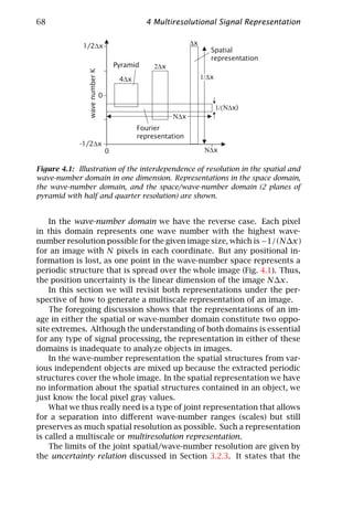
![4.1 Scale in signal processing 69
Table 4.1: Wave number and spatial resolutions of representations of images
in various domains
Domain / Resolution Spatial Wave number Product
resolution resolution
Spatial domain ∆x 1/∆x 1
Wave-number domain N∆x 1/(N∆x) 1
Multiscale domain p∆x 1/(p∆x) 1
product of the resolutions in the spatial and wave-number domain can-
not be beyond a certain threshold. This is exactly what we observed
already in the spatial and wave-number domains. However, besides
these two domains any other combination of resolutions that meets
the uncertainty relation can be chosen. Thus the resolution in wave
numbers, that is, the distinction of various scales in an image, can be
set to any value with a corresponding spatial resolution (Fig. 4.1, Ta-
ble 4.1). As the uncertainty relation gives only the lower limit of the
joint resolution, it is important to devise efficient data structures that
approach this limit.
In the last two decades a number of various concepts have been
developed for multiresolution signal processing. Some trace back to
the early roots of signal processing. This includes various techniques
to filter signals for certain scale ranges such as the windowed Fourier
transform, Gabor filters, polar separable quadrature filters, and filters
steerable in scale (Section 4.2).
Some of these techniques are directly suitable to compute a local
wave number that reflects the dominant scale in a local neighborhood.
Multigrid image structures in the form of pyramids are another early
and efficient multiresolution [1]. More recent developments are the
scale space (Section 4.2) and wavelets [2, 3].
Although all of these techniques seem to be quite different at first
glance, this it not the case. They have much in common; they merely
look at the question of multiresolutional signal representation from a
different point of view. Thus an important issue in this chapter is to
work out the relations between the various approaches.
An early account on multiresolution imaging was given by Rosenfeld
[4]. The standard work on linear scale space theory is by Lindeberg [5]
(see also Chapter 11) and nonlinear scale space theory is treated by
Weickert [6] (see also Chapter 15).](https://image.slidesharecdn.com/computervision-handbookofcomputervisionandapplicationsvolume2-signalprocessingandpatternrecognition-120205081400-phpapp02/85/Computer-vision-handbook-of-computer-vision-and-applications-volume-2-signal-processing-and-pattern-recognition-94-320.jpg)
![70 4 Multiresolutional Signal Representation
4.2 Scale filters
4.2.1 Windowed Fourier transform
One way to a multiresolutional signal representation starts with the
Fourier transform. If the Fourier transform is applied only to a sec-
tion of the image and this section is moved around through the whole
image, then a joint spatial/wave-number resolution is achieved. The
spatial resolution is given by the size of the window and due to the un-
certainty relation (Section 3.2.3) the wave-number resolution is reduced
by the ratio of the image size to the window size. The window function
w(x) must not be a box function. Generally, a useful window func-
tion has a maximum at the origin, is even and isotropic, and decreases
monotonically with increasing distance from the origin. This approach
to a joint space/wave-number representation is the windowed Fourier
transform. It is defined by
∞
2
ˆ
g(x, k0 ) = g(x )w(x − x) exp(−2π ik0 x ) dx (4.1)
−∞
The integral in Eq. (4.1) almost looks like a convolution integral (Sec-
tion 3.2.3). To convert it into a convolution integral we make use of the
fact that the window function is even (w(−k) = w(k)) and rearrange
the second part of Eq. (4.1):
w(x − x) exp(−2π ik0 x ) =
w(x − x ) exp(2π ik0 (x − x )) exp(−2π ik0 x)
Then we can write Eq. (4.1) as a convolution:
ˆ
g(x, k0 ) = [g(x) ∗ w(x) exp(2π ik0 x)] exp(−2π ik0 x) (4.2)
This means that the local Fourier transform corresponds to a convo-
lution with the complex convolution kernel w(x) exp(2π ik0 x) except
for a phase factor exp(−2π ik0 x). Using the shift theorem (Table 3.2),
the transfer function of the convolution kernel can be computed to be
⇒ ˆ
w(x) exp(2π ik0 x) ⇐ w(k − k0 ) (4.3)
This means that the convolution kernel is a bandpass filter with a peak
wave number of k0 . The width of the bandpass is inversely proportional
to the width of the window function. In this way, the spatial and wave-
number resolutions are interrelated to each other. As an example, we
take a Gaussian window function
2
1 |x |2 |k|
w(x) = exp −π 2 ⇒ ˆ
⇐ w(k) = exp −π (4.4)
σD σ σ −2](https://image.slidesharecdn.com/computervision-handbookofcomputervisionandapplicationsvolume2-signalprocessingandpatternrecognition-120205081400-phpapp02/85/Computer-vision-handbook-of-computer-vision-and-applications-volume-2-signal-processing-and-pattern-recognition-95-320.jpg)
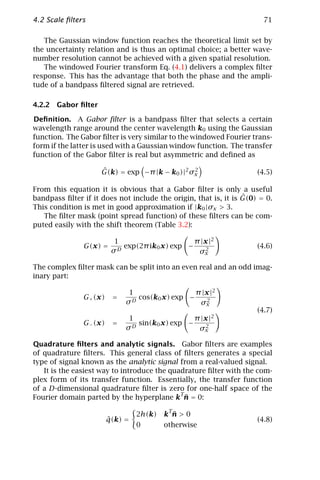
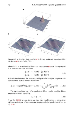
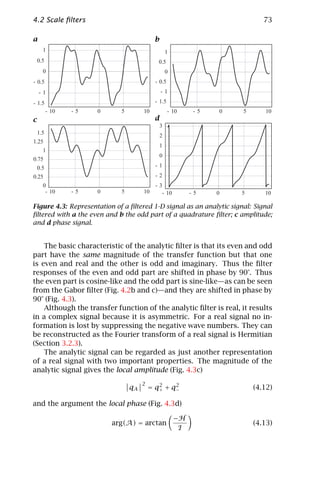
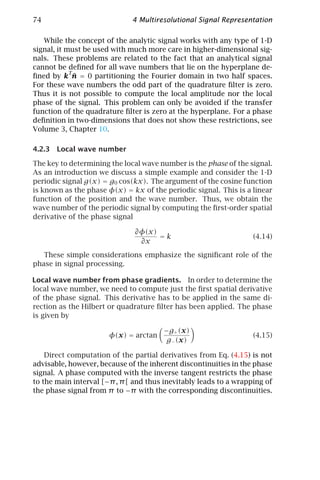
![4.2 Scale filters 75
a b
1 1
1/8 1/4
1/2 0 π /4 π /2 3π / 4
0.8 0.8
0.6 0.6
0.4 0.4
0.2 0.2
0 ~ 1
0
0 0.5 1 1.5 2 2.5 φ 3
0 0.2 0.4 0.6 0.8 k
Figure 4.4: a Radial and b angular part of quadrature filter according to
Eq. (4.17) with l = 2 and B = 2 in different directions and with different peak
wave numbers.
As pointed out by Fleet [7], this problem can be avoided by comput-
ing the phase gradient directly from the gradients of q+ (x) and q− (x):
∂φ(x)
kp =
∂xp
∂
= arctan(−q+ (x)/q− (x)) (4.16)
∂xp
1 ∂q+ (x) ∂q− (x)
= 2 2
q− (x) − q+ (x)
q+ (x) + q− (x) ∂xp ∂xp
This formulation of the phase gradient also eliminates the need for us-
ing trigonometric functions to compute the phase signal and is, there-
fore, significantly faster.
Local wave number from filter ratios. With polar separable quadra-
ˆ
ture filters (ˆ(k)d(φ)) as introduced by Knutsson [8] another scheme
r
for computation of the local scale is possible. These classes of filters
are defined by
(ln k − ln k0 )2
ˆ
r (k) = exp −
(B/2)2 ln 2
(4.17)
cos2l (φ − φk ) |φ − φk | < π /2
ˆ
d(φ) =
0 otherwise
In this equation, the complex notation for quadrature filters is used as
introduced at the beginning of this section. The filter is directed into
the angle φk .
The filter is continuous, as the cosine function is zero in the partition
plane for the two half spaces (|φ − φk | = π /2). The constant k0 denotes
the peak wave number. The constant B determines the half-width of](https://image.slidesharecdn.com/computervision-handbookofcomputervisionandapplicationsvolume2-signalprocessingandpatternrecognition-120205081400-phpapp02/85/Computer-vision-handbook-of-computer-vision-and-applications-volume-2-signal-processing-and-pattern-recognition-100-320.jpg)
![76 4 Multiresolutional Signal Representation
the wave number in number of octaves and l the angular resolution of
the filter. In a logarithmic wave number scale, the filter has the shape of
a Gaussian function. Therefore the radial part has a lognormal shape.
Figure 4.4 shows the radial and angular part of the transfer function.
The lognormal form of the radial part of the quadrature filter sets
is the key for a direct estimate of the local wave number of a narrow-
band signal. According to Eq. (4.17), we can write the radial part of the
transfer function as
(ln k − ln kl )2
ˆ
rl (k) = exp − (4.18)
2σ 2 ln 2
We examine the ratio of the output of two different radial center
frequencies k1 and k2 and obtain:
ˆ
r2 (ln k − ln k2 )2 − (ln k − ln k1 )2
= exp −
ˆ
r1 2σ 2 ln 2
2 2
2(ln k2 − ln k1 ) ln k + ln k2 − ln k1
= exp
2σ 2 ln 2
(ln k2 − ln k1 )[ln k − 1/2(ln k2 + ln k1 )]
= exp
σ 2 ln 2
ln(k/ k2 k1 ) ln(k2 /k1 )
= exp
σ 2 ln 2
ln(k2 /k1 )/(σ 2 ln 2)
k
=
k1 k2
Generally, the ratio of two different radial filters is directly related
to the local wave number. The relation becomes particularly simple if
the exponent in the last expression is one. This is the case, for example,
if the wave number ratio of the two filters is two (k2 /k1 = 2 and σ = 1).
Then
ˆ
r2 k
= (4.19)
ˆ
r1 k1 k2
4.3 Scale space and diffusion
As we have seen with the example of the windowed Fourier transform
in the previous section, the introduction of a characteristic scale adds a
new coordinate to the representation of image data. Besides the spatial
resolution, we have a new parameter that characterizes the current res-
olution level of the image data. The scale parameter is denoted by ξ 1 .
1 In Chapter 11 t is used for the scale parameter. Here we are using ξ in order to
avoid confusion with the time coordinate t for scale spaces of image sequences.](https://image.slidesharecdn.com/computervision-handbookofcomputervisionandapplicationsvolume2-signalprocessingandpatternrecognition-120205081400-phpapp02/85/Computer-vision-handbook-of-computer-vision-and-applications-volume-2-signal-processing-and-pattern-recognition-101-320.jpg)
![4.3 Scale space and diffusion 77
A data structure that consists of a sequence of images with different
resolutions is known as a scale space; we write g(x, ξ) to indicate the
scale space of the image g(x). Such a sequence of images can be gen-
erated by repeated convolution with an appropriate smoothing filter
kernel.
This section is thought as a brief introduction into scale spaces. For
an authoritative monograph on scale spaces, see Lindeberg [5].
4.3.1 General properties of a scale space
In this section, we discuss some general conditions that must be met
by a filter kernel generating a scale space. We will discuss two basic
requirements. First, new details must not be added with increasing
scale parameter. From the perspective of information theory, we may
say that the information content in the signal should continuously de-
crease with the scale parameter.
The second property is related to the general principle of scale in-
variance. This basically means that we can start smoothing the signal
at any scale parameter in the scale space and still obtain the same scale
space.
Minimum-maximum principle. The information-decreasing property
of the scale space with ξ can be formulated mathematically in different
ways. We express it here with the minimum-maximum principle, which
states that local extrema must not be enhanced. This means that the
gray value at a local maximum or minimum must not increase or de-
crease, respectively. For the physical process of diffusion this is an
intuitive property. For example, in a heat transfer problem, a hot spot
must not become hotter or a cool spot cooler.
Semi-group property. The second important property of the scale
space is related to the scale invariance principle. We want to start the
generating process at any scale parameter and still obtain the same
scale space. More quantitatively, we can formulate this property as
B(ξ2 )B(ξ1 ) = B(ξ1 + ξ2 ) (4.20)
This means that the smoothing of the scale space at the scale ξ1 by an
operator with the scale ξ2 is equivalent to the application of the scale
space operator with the scale ξ1 + ξ2 to the original image. Alterna-
tively, we can state that the representation at the coarser level ξ2 can
be computed from the representation at the finer level ξ1 by applying
B(ξ2 ) = B(ξ2 − ξ1 )B(ξ1 ) with ξ2 > ξ1 (4.21)
In mathematics the properties Eqs. (4.20) and (4.21) are referred to as
the semi-group property.](https://image.slidesharecdn.com/computervision-handbookofcomputervisionandapplicationsvolume2-signalprocessingandpatternrecognition-120205081400-phpapp02/85/Computer-vision-handbook-of-computer-vision-and-applications-volume-2-signal-processing-and-pattern-recognition-102-320.jpg)
![78 4 Multiresolutional Signal Representation
Conversely, we can ask what scale space generating kernels exist
that meet both the minimum-maximum principle and the semi-group
property. The answer to this question may be surprising. As shown by
Lindeberg [5, Chapter 2], the Gaussian kernel is the only convolution
kernel that meets both criteria and is in addition isotropic and homo-
geneous. From yet another perspective this feature puts the Gaussian
convolution kernel into a unique position for signal processing. With
respect to the Fourier transform we have already discussed that the
Gaussian function is one of the few functions with a shape that is invari-
ant under the Fourier transform (Section 3.2.4, Table 3.3) and optimal
in the sense of the uncertainty relation (Section 3.2.3). In Section 7.4
we will see in addition that the Gaussian function is the only function
that is separable and isotropic.
4.3.2 Linear scale spaces
Generation by a diffusion process. The generation of a scale space
requires a process that can blur images to a controllable degree. Dif-
fusion is a transport process that tends to level out concentration dif-
ferences. In physics, diffusion processes govern the transport of heat,
matter, and momentum [9] leading to an ever-increasing equalization
of spatial concentration differences. If we identify the time with the
scale parameter ξ, the diffusion process thus establishes a scale space.
To apply a diffusion process to an image, we regard the gray value g
as the concentration of a scalar property. The elementary law of diffu-
sion states that the flux density j is directed against the concentration
gradient g and proportional to it:
j = −D g (4.22)
where the constant D is known as the diffusion coefficient . Using the
continuity equation
∂g
+ j=0 (4.23)
∂t
the diffusion equation is
∂g
= (D g) (4.24)
∂t
For the case of a homogeneous diffusion process (D does not depend
on the position), the equation reduces to
D
∂g ∂2
= D∆g where ∆= 2
(4.25)
∂t ∂xd
d =1](https://image.slidesharecdn.com/computervision-handbookofcomputervisionandapplicationsvolume2-signalprocessingandpatternrecognition-120205081400-phpapp02/85/Computer-vision-handbook-of-computer-vision-and-applications-volume-2-signal-processing-and-pattern-recognition-103-320.jpg)
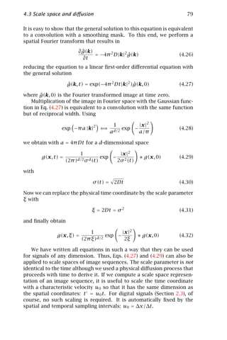
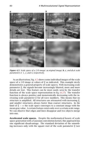
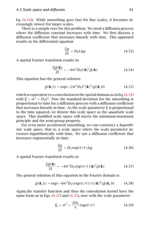
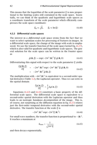
![4.3 Scale space and diffusion 83
4.3.4 Discrete scale spaces
The construction of a discrete scale space requires a discretization of
the diffusion equation and not of the convolution kernel [5]. We start
with a discretization of the 1-D diffusion equation
∂g(x, ξ) ∂ 2 g(x, ξ)
= (4.46)
∂ξ ∂x 2
The derivatives are replaced by discrete differences in the following
way:
∂g(x, ξ) g(x, ξ + ∆ξ) − g(x, ξ)
≈
∂ξ ∆ξ
(4.47)
∂ 2 g(x, ξ) g(x + ∆x, ξ) − 2g(x, ξ) + g(x − ∆x, ξ)
≈
∂x 2 ∆x 2
This leads to the following iteration scheme for computing a discrete
scale space:
g(x, ξ + ∆ξ) = ∆ξg(x + ∆x, ξ) + (1 − 2∆ξ)g(x, ξ) + ∆ξg(x − ∆x, ξ)
(4.48)
or written with discrete coordinates
gn,ξ +1 = ∆ξgn+1,ξ + (1 − 2∆ξ)gn,ξ + ∆ξgn−1,ξ (4.49)
Lindeberg [5] shows that this iteration results in a discrete scale
space that meets the minimum-maximum principle and the semi-group
property if and only if
1
∆ξ ≤ (4.50)
4
The limit case of ∆ξ = 1/4 leads to the especially simple iteration
gn,ξ +1 = 1/4gn+1,ξ + 1/2gn,ξ + 1/4gn−1,ξ (4.51)
Each step of the scale space computation is given by a spatial smoothing
of the signal with the binomial mask B2 = [1/4 1/2 1/4] (Section 7.4).
We can also formulate the general scale space generating operator in
Eq. (4.49) using the convolution operator B. Written in the operator
notation introduced in Section 5.2.3, the operator for one iteration step
to generate the discrete scale space is
(1 − )I + B2 with ≤1 (4.52)
where I denotes the identy operator.](https://image.slidesharecdn.com/computervision-handbookofcomputervisionandapplicationsvolume2-signalprocessingandpatternrecognition-120205081400-phpapp02/85/Computer-vision-handbook-of-computer-vision-and-applications-volume-2-signal-processing-and-pattern-recognition-108-320.jpg)
![84 4 Multiresolutional Signal Representation
This expression is significant, as it can be extended directly to higher
dimensions by replacing B2 with a correspondingly higher-dimensional
smoothing operator. The convolution mask B2 is the simplest mask in
the class of smoothing binomial filters. These filters will be discussed
in Section 7.4. A detailed discussion of discrete linear scale spaces is
given by Lindeberg [5, Chapters 3 and 4].
4.4 Multigrid representations
4.4.1 Basics
The scale space discussed in Section 4.3 has one significant disadvan-
tage. The use of the additional scale parameter adds a new dimension
to the images and thus leads to an explosion of the data storage re-
quirements and, in turn, the computational overhead for generating
the scale space and for analyzing it. Thus, it is not surprising that be-
fore the evolution of the scale space more efficient multiscale storage
schemes, especially pyramids, found widespread application in image
processing. With data structures of this type, the resolution of the im-
ages decreases in such an extent as the scale increases. In this way
an optimum balance between spatial and wave number resolution is
achieved in the sense of the uncertainty relation (Section 3.2.3). Data
structures of this type are known as multiresolution representations [4].
The basic idea is quite simple. While the representation of fine scales
requires the full resolution, coarser scales can be represented at lower
resolution. This leads to a scale space with smaller and smaller im-
ages as the scale parameter increases. In the following two sections
we will discuss the Gaussian pyramid (Section 4.4.2) and the Laplacian
pyramid (Section 4.4.3) as efficient discrete implementations of dis-
crete scale spaces. In addition, while the Gaussian pyramid constitutes
a standard scale space, the Laplacian pyramid is a discrete version of a
differential scale space (Section 4.3.3).
4.4.2 Gaussian pyramid
When subsampling an image, for example, by taking every second pixel
in every second line it is important to consider the sampling theorem
(Section 2.4.2). Before subsampling, the image must be smoothed to an
extent that no aliasing occurs in the subsampled image. Consequently,
for subsampling by a factor two, we must ensure that all structures,
which are sampled less than four times per wavelength, are suppressed
by an appropriate smoothing filter. This means that size reduction
must go hand-in-hand with appropriate smoothing.](https://image.slidesharecdn.com/computervision-handbookofcomputervisionandapplicationsvolume2-signalprocessingandpatternrecognition-120205081400-phpapp02/85/Computer-vision-handbook-of-computer-vision-and-applications-volume-2-signal-processing-and-pattern-recognition-109-320.jpg)
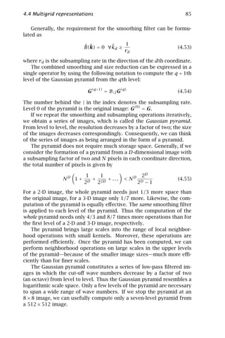
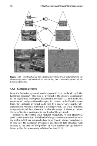
![4.4 Multigrid representations 87
The differentiation in scale direction in the continuous scale space
is approximated by subtracting two levels of the Gaussian pyramid in
the discrete scale space. In order to do so, first the image at the coarser
level must be expanded. This operation is performed by an expansion
operator E↑2 . As with the reducing smoothing operator, the degree of
expansion is denoted by the figure after the ↑ in the index.
The expansion is significantly more difficult than the size reduction
because the missing information must be interpolated. For a size in-
crease of two in all directions, first every second pixel in each row must
be interpolated and then every second row. Interpolation is discussed
in detail in Chapter 8. With the introduced notation, the generation of
the pth level of the Laplacian pyramid can be written as:
(p) (p +1)
L(p) = G − E ↑2 G (4.56)
The Laplacian pyramid is an effective scheme for a bandpass decom-
position of an image. The center wave number is halved from level to
level. The last image of the Laplacian pyramid is a low-pass-filtered
image containing only the coarsest structures.
The Laplacian pyramid has the significant advantage that the origi-
nal image can be reconstructed quickly from the sequence of images in
the Laplacian pyramid by recursively expanding the images and sum-
ming them up. In a Laplacian pyramid with p + 1 levels, the level p
(counting starts with zero!) is the coarsest level of the Gaussian pyra-
mid. Then the level p − 1 of the Gaussian pyramid can be reconstructed
by
G(p−1) = L(p−1) + E↑2 Gp (4.57)
Note that this is just the inversion of the construction scheme for the
Laplacian pyramid. This means that even if the interpolation algo-
rithms required to expand the image contain errors, they affect only the
Laplacian pyramid and not the reconstruction of the Gaussian pyramid
from the Laplacian pyramid, because the same algorithm is used. The
recursion in Eq. (4.57) is repeated with lower levels until level 0, that is,
the original image, is reached again. As illustrated in Fig. 4.6, finer and
finer details become visible during the reconstruction process.
The Gaussian and Laplacian pyramids are examples of multigrid
data structures, which were introduced into digital image processing
in the early 1980s and since then have led to a tremendous increase in
speed of image processing algorithms. A new research area, multireso-
lutional image processing, was established by Rosenfeld [4].](https://image.slidesharecdn.com/computervision-handbookofcomputervisionandapplicationsvolume2-signalprocessingandpatternrecognition-120205081400-phpapp02/85/Computer-vision-handbook-of-computer-vision-and-applications-volume-2-signal-processing-and-pattern-recognition-112-320.jpg)
![88 4 Multiresolutional Signal Representation
a b
0.6 0.6
0.4 0.4
~
0.2 0.2
~
0 ky 0 ky
-0.4 0 -0.4 0
-0.2 -0.2
-0.2 -0.2
0 0
0.2 ~ -0.4 0.2 ~ -0.4
kx kx
0.4 0.4
c
0.6
0.4
~
0.2
0 ky
-0.4 0
-0.2
-0.2
0
0.2 ~ -0.4
kx
0.4
Figure 4.7: Pseudo 3-D plots of the directio-pyramidal decomposition according
to Eq. (4.60): a directional bandpass filter in x direction; b directional bandpass
filter in y direction; c isotropic bandpass filter, sum of a and b.
4.4.4 Directio-pyramidal decomposition
The Laplacian pyramid decomposes an image in logarithmic wave num-
ber intervals one octave (factor 2) distant. A useful extension is the ad-
ditional decomposition into different directions. Such a decomposition
is known as directio-pyramidal decomposition [10]. This decomposition
should have the same properties as the Laplacian pyramid: the addi-
tion of all partial images should give the original. This implies that
each level of the Laplacian pyramid must be decomposed into several
directional components. An efficient scheme for decomposition into
two directional components is as follows. The smoothing is performed
by separable smoothing filters followed by a subsampling operator R↓2 ,
taking only each second pixel in each second line,
G(1) = R↓2 Bx By G(0) (4.58)
The first level of the Laplacian pyramid then is
(0) (1)
L=G − E ↑2 G (4.59)
Then, the two directional components are given by
(0)
L1 = 1/2(L − (Bx − By )G )
(0) (4.60)
L2 = 1/2(L + (Bx − By )G )](https://image.slidesharecdn.com/computervision-handbookofcomputervisionandapplicationsvolume2-signalprocessingandpatternrecognition-120205081400-phpapp02/85/Computer-vision-handbook-of-computer-vision-and-applications-volume-2-signal-processing-and-pattern-recognition-113-320.jpg)
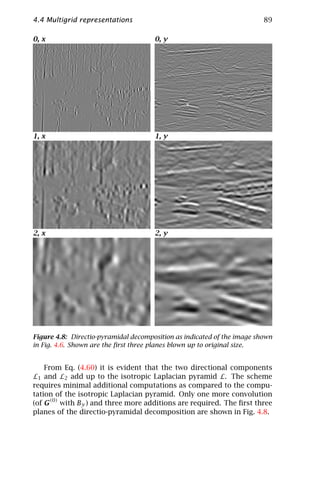
![90 4 Multiresolutional Signal Representation
4.5 References
[1] Burt, P. J., (1984). The pyramid as a structure for efficient computation. In
Multiresolution Image Processing and Analysis, A. Rosenfeld, ed., Vol. 12
of Springer Series in Information Sciences, pp. 6–35. New York: Springer.
[2] Meyer, Y., (1993). Wavelets: Algorithms & Applications. Philadelphia:
SIAM.
[3] Kaiser, G., (1994). A Friendly Guide to Wavelets. Boston, MA: Birkhäuser.
[4] Rosenfeld, A. (ed.), (1984). Multiresolution Image Processing and Analysis.
New York: Springer.
[5] Lindeberg, T., (1994). Scale-space Theory in Computer Vision. Boston:
Kluwer Academic Publishers.
[6] Weickert, J., (1998). Anisotropic Diffusion in Image Processing. Stuttgart:
Teubner-Verlag.
[7] Fleet, D. J., (1990). Measurement of Image Velocity. Diss., University of
Toronto.
[8] Knutsson, H., (1982). Filtering and Reconstruction in Image Processing.
Diss., Linköping Univ.
[9] Crank, J., (1975). The Mathematics of Diffusion. 2nd edition. New York:
Oxford University Press.
[10] Jähne, B., (1987). Image sequence analysis of complex physical objects:
nonlinear small scale water surface waves. In Proceedings ICCV’87, Lon-
don, pp. 191–200, IEEE. Washington, DC: IEEE Computer Society Press.](https://image.slidesharecdn.com/computervision-handbookofcomputervisionandapplicationsvolume2-signalprocessingandpatternrecognition-120205081400-phpapp02/85/Computer-vision-handbook-of-computer-vision-and-applications-volume-2-signal-processing-and-pattern-recognition-115-320.jpg)

![94 5 Neighborhood Operators
5.1 Introduction
The extraction of features from multidimensional signals requires the
analysis of at least a local neighborhood. It is obvious that any process-
ing of individual pixels, so-called point operations, will be of no use for
this task. Such operations are just “cosmetics,” changing the visual im-
pression of the image but not extracting any useful information. By
analysis of the local neighborhood a rich set of features can already be
extracted. We can distinguish areas of constant gray values from those
that contain an edge, a texture, or just noise.
Thus this chapter gives an important theoretical basis for lowlevel
signal processing. We first discuss some basics, provide a general def-
inition of neighborhood operators and introduce a useful operator no-
tation (Section 5.2.3). The main part of the chapter is devoted to a
detailed discussion of the various classes of neighborhood operators:
linear shift-invariant operators or convolution operators (Section 5.3),
and various classes of nonlinear operators (Section 5.5). In this respect
we will also discuss the principal limitations of linear operators in Sec-
tion 5.5.1. The last section of the chapter (Section 5.6) focuses on more
practical questions. Can we establish some general rules as to how
to compute neighborhood operators in an efficient way? How do we
handle neighborhood operators at the borders of images?
5.2 Basics
5.2.1 Definition of neighborhood operators
A neighborhood operator takes the gray values of the neighborhood
around a point, performs some operations with them, and writes the
result back on the pixel. This operation is repeated for all points of
the signal. Therefore, we can write a neighborhood operation with a
multidimensional continuous signal g(x) as
g (x) = N({g(x )}, ∀(x − x ) ∈ M) (5.1)
where M is an area, called mask, region of support , or structure element .
The size and shape of M determines the neighborhood operation by
specifying the input values of g in the area M shifted with its origin to
the point x. The neighborhood operation N itself is not specified here.
It can be of any type; its result determines the value of the output g
at x. For symmetry reasons the mask is often symmetric and has its
center of gravity in the origin.
For digital signals a general neighborhood operation can be expressed
as
Gm,n = N(Gm −m,n −n }, ∀ [m, n]T ∈ M) (5.2)](https://image.slidesharecdn.com/computervision-handbookofcomputervisionandapplicationsvolume2-signalprocessingandpatternrecognition-120205081400-phpapp02/85/Computer-vision-handbook-of-computer-vision-and-applications-volume-2-signal-processing-and-pattern-recognition-119-320.jpg)
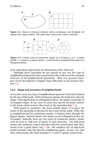
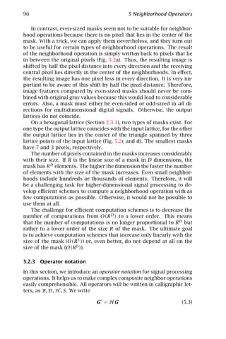
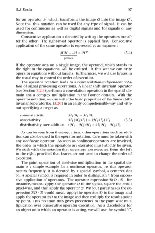
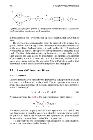
![5.3 Linear shift-invariant filters 99
5.3.2 Shift invariance and convolution
Another important property of an operator is shift invariance or homo-
geneity. It means that the response of the operator does not explicitly
depend on the position. If we shift a signal, the output image is the
same but for the shift applied. We can formulate this property more
elegantly with a shift operator S. For 2-D images, for example, the shift
operator is defined as
mn
SGm n = Gm −m,n −n (5.8)
An operator is then shift-invariant if and only if it commutes with the
shift operator, that is,
H S = SH (5.9)
Note that the shift operator S itself is a shift-invariant operator. An
operator that is both linear and shift invariant is known as a linear
shift-invariant operator or short LSI operator. This important class of
operators is also known as linear time-invariant or LTI operators for
time series.
It can be proven [1] that a linear shift-invariant operator must nec-
essarily be a convolution operation in the space domain. There is no
other operator type that is both linear and shift invariant. Thus, linear
shift-invariant neighborhood operators share all the useful features of
convolution that were discussed in Section 3.2.3. They are commuta-
tive, associative, and distribute over addition (see also Eq. (5.5)). These
properties are very useful for an efficient design of filter operations
(Chapter 6).
5.3.3 Point spread function
As just discussed in the previous section, an LSI filter can be repre-
sented in the space domain as a convolution operation. In two dimen-
sions the image G is convolved with another image H that represents
the LSI operator:
M −1 N −1
Gmn = Hm ,n Gm−m ,n−n (5.10)
m =0 n =0
Since for a neighborhood operation H is zero except for a small neigh-
borhood this operation can also be written as
R R
Gmn = H−m ,−n Gm+m ,n+n (5.11)
m =−R n =−R](https://image.slidesharecdn.com/computervision-handbookofcomputervisionandapplicationsvolume2-signalprocessingandpatternrecognition-120205081400-phpapp02/85/Computer-vision-handbook-of-computer-vision-and-applications-volume-2-signal-processing-and-pattern-recognition-124-320.jpg)
![100 5 Neighborhood Operators
In this equation it is assumed that coefficients of H are nonzero only
in a (2R+1) × (2R+1) window. Both representations are equivalent if we
consider the periodicity in the space domain (Section 3.3.1). The latter
representation is much more practical and gives a better comprehen-
sion of the operator. For example, the following M × N matrix and 3 × 3
filter mask are equivalent:
0• −1 0 . . . 0 1
1 0 0 ... 0 2
0 0 0 ... 0 0 0 − 1 −2
. . . . . . ≡ 1 0 • −1 (5.12)
. . . . . .
. . . . . .
2 1 0
0 0 0 ... 0 0
−1 − 2 0 . . . 0 0
For a D dimensional signal, the convolution sum can be written with
a simplified vector indexing also used in Section 2.4.4:
R
Gn = H−n Gn+n (5.13)
n =−R
with n = [n1 , n2 , . . . , nD ], R = [R1 , R2 , . . . , RD ], where Gn is an element
of a D-dimensional signal Gn1 ,n2 ,... ,nD . The notation for the sums in this
equation is an abbreviation for
R R1 R2 RD
= ... (5.14)
n =−R n1 =−R1 n2 =−R2 nD =−RD
The vectorial indexing introduced here allows writing most of the rela-
tions for arbitary dimensional signals in a simple way. Moreover, it can
also be used for skewed coordinate systems if n are regarded as the in-
dices of the corresponding lattice vectors (see Eq. (2.27), Section 2.4.2).
The filter mask is identical to another quantity known as the point
spread function, which gives the response of the filter to a point image:
R
Pn = Hn Pn−n = Hn (5.15)
n =−R
where
1 n=0
Pn = (5.16)
0 otherwise
The central importance of the point spread function is based on the
fact that the convolution operation is linear. If we know the response](https://image.slidesharecdn.com/computervision-handbookofcomputervisionandapplicationsvolume2-signalprocessingandpatternrecognition-120205081400-phpapp02/85/Computer-vision-handbook-of-computer-vision-and-applications-volume-2-signal-processing-and-pattern-recognition-125-320.jpg)
![5.3 Linear shift-invariant filters 101
to a point image, we can compute the response to any image, as any
image can be composed of point images as discussed in Section 3.1.1.
With respect to the analysis of time series, the point spread function is
known as the impulse response, with respect to the solution of partial
differential equations as the Green’s function [2].
5.3.4 Transfer function
The Fourier transform of the convolution mask is known as the trans-
fer function of a linear filter. The transfer function has an important
practical meaning. For each wave number, it gives the factor by which
a periodic structure is multiplied using the filter operation. This factor
is generally a complex number. Thus, a periodic structure experiences
not only a change in the amplitude but also a phase shift:
ˆ ˆ ˆ
Gv = Hv Gv = rH exp(iϕH ) rG exp(iϕG )
(5.17)
= rH rG exp[i(ϕH + ϕG )]
where the complex numbers are represented by their magnitude and
phase as complex exponentials.
Using the wave number normalized to the Nyquist limit (Eq. (2.34)
in Section 2.4.2), the transfer function is given by
R
ˆ ˜
h(k) = ˜
hn exp(−π in k) (5.18)
n =−R
for a 1-D signal and by
R
ˆ ˜
h(k) = ˜
Hn exp(−π in T k) (5.19)
n =−R
for a multidimensional signal. For a nonorthogonal, that is, skewed
lattice, the vectorial index n has to be replaced by the reciprocal lattice
vector (Eq. (2.29)), and Eq. (5.19) becomes
R
ˆ
h(k) = rT
Hr exp(−2π iˆv k) (5.20)
v =−R
5.3.5 Symmetries
Symmetries play a central rule for linear shift-invariant filters in the
processing of higher-dimensional signal processing. This is because
of the simplified transfer function of symmetric masks. According to
Section 3.2.3, filters of even and odd symmetry have a real and purely](https://image.slidesharecdn.com/computervision-handbookofcomputervisionandapplicationsvolume2-signalprocessingandpatternrecognition-120205081400-phpapp02/85/Computer-vision-handbook-of-computer-vision-and-applications-volume-2-signal-processing-and-pattern-recognition-126-320.jpg)
![102 5 Neighborhood Operators
imaginary transfer function, respectively. The symmetry of a filter is
most generally expressed by:
HR−r = ±Hr (5.21)
This is a necessary and sufficient condition for a real or imaginary trans-
fer function. Filters normally meet a stronger symmetry condition for
each direction d:
Hr1 ,... ,Rd −rd ,... ,rD = ±Hr1 ,... ,rd ,... ,rD (5.22)
For separable symmetric filters, the symmetry conditions can be
expressed for each 1-D component separately:
hRd −rd = ±hrd (5.23)
As the transfer functions of the 1-D components of separable filters
are combined multiplicatively, an even and odd number of odd compo-
nents results in an even and odd filter according to Eq. (5.21) and thus
into a real and imaginary transfer function, respectively.
Because of the significance of separable filters (Section 5.6.1), we
focus on the symmetry of 1-D filters. Besides odd and even symmetry,
it is necessary to distinguish filters with an even and odd number of
coefficients.
The situation is straightforward for filters with an odd number of
coefficients. Then the central coefficient is the center of symmetry and
the result of a filter operation is written to the position of this central
coefficient. This symmetry is implicitly considered in Eqs. (5.13) and
(5.18) where the central coefficient has the index 0. With this indexing
of the filter coefficients, the convolution sum and transfer function of
even 1-D filters with 2R + 1 coefficients—also known as type I FIR filter
[3]—can be expressed as
R R
gn = h0 gn + hn (gn+n + gn−n ), ˆ ˜
h(k) = h0 + ˜
2hn cos(n π k)
n =1 n =1
(5.24)
and for odd filters with 2R + 1 coefficients or type III FIR filters as
R R
gn = hn (gn−n − gn+n ), ˆ ˜
h(k) = i ˜
2hn sin(n π k) (5.25)
n =1 n =1
For filters with an even number of coefficients, there is no central
pixel. The symmetry center rather lies in-between two pixels. This
means that the results of a filter operation with such a filter are to be
placed on a grid that is shifted by half a pixel distance. Because of](https://image.slidesharecdn.com/computervision-handbookofcomputervisionandapplicationsvolume2-signalprocessingandpatternrecognition-120205081400-phpapp02/85/Computer-vision-handbook-of-computer-vision-and-applications-volume-2-signal-processing-and-pattern-recognition-127-320.jpg)
![5.3 Linear shift-invariant filters 103
this shift between the output pixel and the input pixels, the transfer
function of an even filter with 2R coefficients type II FIR filter is
R
ˆ ˜
h(k) = h0 + ˜
2hn cos((n − 1/2)π k) (5.26)
n =1
The transfer function of an odd filter with 2R coefficients or type IV FIR
filter is
R
ˆ ˜
h(k) = i ˜
2hn sin((n − 1/2)π k) (5.27)
n =1
The equations for symmetric filters for two and more dimensions
are significantly more complex and are discussed in Jähne [4].
5.3.6 LSI operators as least squares estimators
LSI operators compute a new value at each point in a signal from a linear
combination of neighboring points. Likewise, a least squares estimator
computes the estimate of a quantity from a linear combination of the
input values. Thus it appears that a close relationship should exist
between LSI operators and least squares estimators.
We assume that we want to fit a certain function with linear param-
eters ap
P −1
f (x) = ap fp (x) (5.28)
p =0
to the local spatial gray value variation g(x). For 2-D digital signals,
the continuous functions fp (x) have to be replaced by matrices F p .
All of the following equations are also valid for digital signals but it is
more convenient to stick with the continuous case. In the least squares
sense, the following error measure e2 (x) should be minimized:
∞ 2
P −1
e2 (x) = w(x ) ap (x)fp (x ) − g(x + x ) dDx (5.29)
−∞ p =0
In this integral the window function w(x ) has been introduced to limit
the fit to a local neighborhood around the point x. Therefore, the
fit coefficients ap (x) depend on the position. Normally, the window
function is an isotropic even function with a maximum at the origin
monotonically decreasing with increasing distance from the origin. We
further assume that the window function is normalized, that is,
∞
w(x ) dDx = 1 (5.30)
−∞](https://image.slidesharecdn.com/computervision-handbookofcomputervisionandapplicationsvolume2-signalprocessingandpatternrecognition-120205081400-phpapp02/85/Computer-vision-handbook-of-computer-vision-and-applications-volume-2-signal-processing-and-pattern-recognition-128-320.jpg)
![104 5 Neighborhood Operators
For the sake of simpler equations, the following abbreviations will be
used in this section:
∞
f p gx = w(x )fp (x )g(x + x ) dDx
−∞
∞
(5.31)
fp fq = w(x )fp (x )fq (x ) dDx
−∞
Setting all derivatives of Eq. (5.29) with respect to the parameters ap (x)
zero, the following linear equation system is obtained as the standard
least squares solution of the minimization problem
a(x) = M −1 d(x) (5.32)
with
T
Mp,q = fp fq , a = [a0 (x), a1 (x), . . . , aP −1 (x)] d p = fp g x
The solution of Eq. (5.32) becomes most simple if the functions fp (x)
2
are orthogonal to each other, that is, fp fq = fp δp−q . Then the
matrix M is diagonal and
2
ap (x) = fp gx fp (5.33)
This expression can also be written as convolution integral by using
Eq. (5.31) and substituting x by −x :
∞
ap (x) = w(x )fp (−x )g(x − x ) dDx (5.34)
−∞
This means that the fit coefficient for each point is computed by con-
volving the windowed and mirrored orthonormal function with the sig-
nal.
Example 5.1: Plane fit
As a simple example we discuss the local plane fit, that is, the local
approximation of the gray scale variation by a plane. The fit function
is
f (x) = a0 + a1 x1 + a2 x2 , f0 = 1, f1 = x1 , f2 = x2 (5.35)](https://image.slidesharecdn.com/computervision-handbookofcomputervisionandapplicationsvolume2-signalprocessingandpatternrecognition-120205081400-phpapp02/85/Computer-vision-handbook-of-computer-vision-and-applications-volume-2-signal-processing-and-pattern-recognition-129-320.jpg)
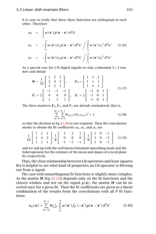
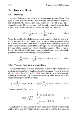
![5.4 Recursive filters 107
can have zeros. Thus the nonrecursive part of the transfer function
may cause zeros and the recursive part poles.
A deeper analysis of the zeros and thus the structure of the trans-
fer function is not possible in the form as Eq. (5.44) is written. It re-
quires an extension similar to the extension from real numbers to com-
plex numbers that was necessary to introduce the Fourier transform
(Section 3.1.3). We observe that the expressions for both the numer-
ator and the denominator are polynomials in the complex exponential
exp(2π ik). The complex exponential has a magnitude of one and thus
covers the unit circle in the complex plane. It covers the whole complex
plane if we add a radius r to the expression: z = r exp(2π ik).
With this extension, the expressions become polynomials in z. As
such we can apply the fundamental law of algebra that any complex
polynomial of degree n can be factorized in n factors containing the
roots or zeros of the polynomial. Thus we can write a new expression
in z, which becomes the transfer function for z = exp(2π ik):
R
(1 − cn z−1 )
ˆ n =−R
h(z) = S
(5.45)
(1 − dn z −1 )
n =0
Each of the factors cn and dn is a zero of the according polynomial
(z = cn or z = dn ).
The inclusion of the factor r in the extended transfer function re-
sults in an extension of the Fourier transform, the z-transform that is
defined as
∞
ˆ
g(z) = gn z−n (5.46)
n=−∞
The z-transform of the series gn can be regarded as the Fourier trans-
form of the series gn r −n [5]. The z-transform is the key mathemat-
ical tool to understand recursive filters. Detailed accounts of the z-
transform are given by Oppenheim and Schafer [3] and Poularikas [6];
the 2-D z-transform is discussed by Lim [5].
The factorization of the z-transform of the filter in Eq. (5.45)—and in
turn of the transfer function—is an essential property. Multiplication
of the individual factors of the transfer function means that we can
decompose any filter into elementary filters containing only one factor
because multiplication of transfer functions is equivalent to cascaded
convolution in the spatial domain (Section 3.2.3). The basic filters that
are equivalent to a single factor in Eq. (5.45) will be discussed further
in Section 5.4.6.](https://image.slidesharecdn.com/computervision-handbookofcomputervisionandapplicationsvolume2-signalprocessingandpatternrecognition-120205081400-phpapp02/85/Computer-vision-handbook-of-computer-vision-and-applications-volume-2-signal-processing-and-pattern-recognition-132-320.jpg)
![108 5 Neighborhood Operators
Recursive filters can also be defined in higher dimensions with the
same type of equations as in Eq. (5.42); also the transfer function and
z-transform of higher dimensional recursive filters can be written in
the very same way as in Eq. (5.44). However, it is generally not possi-
ble to factorize the z-transform as in Eq. (5.45) [5]. From Eq. (5.45) we
can immediately conclude that it will be possible to factorize a sepa-
rable recursive filter because then the higher dimensional polynomials
can be factorized into 1-D polynomials. Given these inherent difficul-
ties of higher-dimensional recursive filters we will restrict the further
discussion on 1-D recursive filters that can be extended by cascaded
convolution into higher-dimensional filters.
5.4.3 Infinite and unstable response
The impulse response or point spread function of a recursive filter is no
longer identical to the filter coefficients as for nonrecursive filters (Sec-
tion 5.3.3). It must rather be computed as the inverse Fourier transform
of the transfer function. The impulse response of nonrecursive filters
has only a finite number of nonzero samples. A filter with this prop-
erty is called a finite-duration impulse response or FIR filter. In contrast,
recursive filters have an infinite-duration impulse response (IIR).
The stability of the filter response is not an issue for nonrecursive fil-
ters but of central importance for recursive filters. A filter is said to be
stable if and only if each bound input sequence generates a bound out-
put sequence. In terms of the impulse response this means that a filter
is stable if and only if the impulse response is absolutely summable [3].
For 1-D filters the analysis of the stability is straightforward because
the conditions are well established by same basic algebraic theorems.
A filter is stable and causal if and only if all poles and zeros of the
ˆ
z-transform h(z) (Eq. (5.45)) are inside the unit circle [3].
5.4.4 Relation between recursive and nonrecursive filters
Any stable recursive filter can be replaced by a nonrecursive filter, in
general with an infinite-sized mask. Its mask is given by the point
spread function of the recursive filter. In practice, the masks cannot
be infinite and also need not be infinite. This is due to the fact that the
envelope of the impulse response of any recursive filter decays expo-
nentially (Section 5.4.6).
Another observation is of importance. From Eq. (5.44) we see that
the transfer function of a recursive filter is the ratio of its nonrecursive
and recursive part. This means that a purely recursive and a nonrecur-
sive filter with the same coefficients are inverse filters to each other.
This general relation is a good base to construct inverse filters from
nonrecursive filters.](https://image.slidesharecdn.com/computervision-handbookofcomputervisionandapplicationsvolume2-signalprocessingandpatternrecognition-120205081400-phpapp02/85/Computer-vision-handbook-of-computer-vision-and-applications-volume-2-signal-processing-and-pattern-recognition-133-320.jpg)
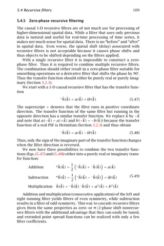

![5.4 Recursive filters 111
a b
.1/2
.3/4 -1/2
7/8
15/16 -1/4
-1/8
31/32
-1/16
~ ~
log k k
Figure 5.4: Transfer function of the relaxation filter gn = αgn 1 + (1 − α)gn
applied first in forward and then in backward direction for a positive; and b
negative values of α as indicated.
From this transfer function, we can compute the multiplicative (ˆ) ap-
r
plication of the filters by running it successively in positive and negative
direction, see Eq. (5.49):
(1 − α)2 1
ˆ ˜
r (k) = = (5.55)
˜
1 − 2α cos π k + α2 ˜
1 + β − β cos π k
with
2α 1 + β − 1 + 2β
β= and α=
(1 − α)2 β
From Eq. (5.53) we can conclude that the relaxation filter is stable if
|α| < 1, which corresponds to β ∈] − 1/2, ∞[. As already noted, the
˜
transfer function is one for small wave numbers. A Taylor series in k
results in
α α((1 + 10α + α2 )
ˆ ˜
r (k) ≈= 1 − 2
˜
(π k)2 + ˜
(π k)4 (5.56)
(1 − α) 12(1 − α2 )2
If α is positive, the filter is a low-pass filter (Fig. 5.4a). It can be tuned by
adjusting α. If α is approaching 1, the averaging distance becomes infi-
nite. For negative α, the filter enhances high wave numbers (Fig. 5.4b).
This filter is the discrete analog to the first-order differential equa-
˙
tion y + τy = 0 describing a relaxation process with the relaxation time
τ = −∆t/ ln α [4].
Resonance filter. The transfer function of a filter with a pair of complex-
conjugate zeros running in forward or backward direction is
±
ˆ ˜
s (k) = ˜
1
˜ ·
1
˜ ˜
1−r exp(iπ k0 ) exp( iπ k) 1−r exp(−iπ k0 ) exp( iπ k)
(5.57)
1
= ˜ ˜ ˜
1−2r cos(π k0 ) exp( iπ k)+r 2 exp( 2iπ k)](https://image.slidesharecdn.com/computervision-handbookofcomputervisionandapplicationsvolume2-signalprocessingandpatternrecognition-120205081400-phpapp02/85/Computer-vision-handbook-of-computer-vision-and-applications-volume-2-signal-processing-and-pattern-recognition-136-320.jpg)
![112 5 Neighborhood Operators
a b
0.1 0.3 0.5 0.7 0.9
.1/2
.3/4
7/8
15/16
~ ~
k k
Figure 5.5: Transfer function of the zero-phase recursive resonance filter for
˜ ˜
a k0 = 1/2 and values of r as indicated; and b r = 7/8 and values of k0 as
indicated.
The second row of the equation shows that this is the transfer function
of the recursive filter
˜
gn = gn + 2r cos(π k0 )gn − r 2 gn (5.58)
1 2
The impulse response of this filter is [3]
rn ˜
sin[(n + 1)π k0 ] n ≥ 0
h±n = ˜
sin π k0 (5.59)
0 n<0
If we run the filter back and forth, the resulting transfer function is
ˆ ˜
s (k) = ˜ ˜
1
˜ ˜
(5.60)
1−2r cos[π (k−k0 )]+r 2 1−2r cos[π (k+k0 )]+r 2
From this equation, it is evident that this filter is a bandpass filter with
˜
a center wave number of k0 . The parameter r is related to the width of
˜ ˜
the bandpass. If r = 1, the transfer function has two poles at k = ±k0 .
If r > 1, the filter is unstable; even the slightest excitement will cause
infinite amplitudes of the oscillation. The filter is only stable for r ≤ 1.
The response of this filter can be normalized to obtain a bandpass
filter with a unit response at the center wave number. The transfer
function of this normalized filter is
˜
(1−r 2 )2 sin2 (π k0 )
ˆ ˜
s (k) = ˜ ˜ ˜ ˜ (5.61)
(1+r 2 )2 +2r 2 cos(2π k0 )−4r (1+r 2 ) cos(π k0 ) cos(π k)+2r 2 cos(2π k)
The denominator in Eq. (5.61) is still the same as in Eq. (5.60); it has only
˜
been expanded in terms with cos(nπ k0 ). The corresponding recursive
filter coefficients are:
˜ ˜
gn = (1 − r 2 ) sin(π k0 )gn + 2r cos(π k0 )gn − r 2 gn (5.62)
1 2](https://image.slidesharecdn.com/computervision-handbookofcomputervisionandapplicationsvolume2-signalprocessingandpatternrecognition-120205081400-phpapp02/85/Computer-vision-handbook-of-computer-vision-and-applications-volume-2-signal-processing-and-pattern-recognition-137-320.jpg)
![5.5 Classes of nonlinear filters 113
˜
Figure 5.5 shows the transfer function of this filter for values of k0 and
r as indicated.
For symmetry reasons, the factors become most simple for a reso-
˜
nance wave number of k0 = 1/2. Then the recursive filter is
gn = (1 − r 2 )gn − r 2 gn 2 = gn − r 2 (gn + gn 2) (5.63)
with the transfer function
(1 − r 2 )2
ˆ ˜
s (k) = (5.64)
˜
1 + r 4 + 2r 2 cos(2π k)
˜
The maximum response of this filter at k = 1/2 is one and the minimum
response at k˜ = 0 and k = 1 is ((1 − r 2 )/(1 + r 2 ))2 .
˜
This resonance filter is the discrete analog to a linear system gov-
erned by the second-order differential equation y + 2τ y + ω2 y = 0, the
¨ ˙ 0
damped harmonic oscillator. The circular eigenfrequency ω0 and the
time constant τ of a real-world oscillator are related to the parameters
˜
of the discrete oscillator, r and k0 by [4]
r = exp(−∆t/τ) and ˜
k0 = ω0 ∆t/π (5.65)
5.5 Classes of nonlinear filters
5.5.1 Limitations of linear filters
In the previous sections, the theory of linear shift-invariant filters was
discussed in detail. Although the theory of these filters is well estab-
lished and they can be applied, they still have some severe limitations.
Basically, linear filters cannot distinguish between a useful feature and
noise. This property can be best demonstrated with a simple example.
We assume a simple signal model with additive noise:
⇒ ˆ ˆ ˆ
g (x) = g(x) + n(x) ⇐ g (k) = g(k) + n(k) (5.66)
ˆ ˆ
The signal to noise ratio (SNR) is defined by g(k) / n(k) . If we now
ˆ
apply a linear filter with the transfer function h(k) to this signal, the
filtered signal is
ˆ ˆ ˆ ˆ ˆ ˆ ˆ ˆ ˆ
h(k)g (k) = h(k)(g(k) + n(k)) = h(k)g(k) + h(k)n(k) (5.67)
It is immediately evident that the noise and the signal are damped by
the same factor. Consequently, the SNR does not increase at all by
linear filtering, it just stays the same.
From the preceding considerations, it is obvious that more complex
approaches are required than linear filtering. Common to all these ap-
proaches is that in one or the other way the filters are made dependent](https://image.slidesharecdn.com/computervision-handbookofcomputervisionandapplicationsvolume2-signalprocessingandpatternrecognition-120205081400-phpapp02/85/Computer-vision-handbook-of-computer-vision-and-applications-volume-2-signal-processing-and-pattern-recognition-138-320.jpg)
![114 5 Neighborhood Operators
on the context or are tailored for specific types of signals. Often a con-
trol strategy is an important part of such filters that controls which
filter or in which way a filter has to be applied at a certain point in
the image. Here, we will outline only the general classes for nonlinear
filters. Pitas and Venetsanopoulos [7] give a detailed survey on this
topic.
5.5.2 Rank-value filters
Rank-value filters are based on a quite different concept than linear-
shift invariant operators. These operators consider all pixels in the
neighborhood. It is implicitly assumed that each pixel, distorted or
noisy, carries still useful and correct information. Thus, convolution
operators are not equipped to handle situations where the value at a
pixel carries incorrect information. This situation arises, for instance,
when an individual sensor element in a CCD array is defective or a
transmission error occurred.
To handle such cases, operations are required that apply selection
mechanisms and do not use all pixels in the neighborhood to compute
the output of the operator. The simplest class of operators of this
type are rank-value filters. While the convolution operators may be
characterized by “weighting and accumulating,” rank-value filters may
be characterized by “comparing and selecting.”
For this we take all the gray values of the pixels which lie within the
filter mask and sort them by ascending gray value. This sorting is com-
mon to all rank-value filters. They only differ by the position in the list
from which the gray value is picked out and written back to the center
pixel. The filter operation that selects the medium value is called the
median filter . The median filter is an excellent example for a filter that
is adapted to a certain type of signal. It is ideally suited for removing
a single pixel that has a completely incorrect gray value because of a
transmission or data error. It is less well suited, for example, to reduce
white noise.
Other known rank-value filters are the minimum filter and the max-
imum filter . As the names say, these filters select out of a local neigh-
borhood, either the minimum or the maximum gray value forming the
base for gray scale morphological filters (Chapter 21).
As rank-value filters do not perform arithmetic operations but select
pixels, we will never run into rounding problems. These filters map a
discrete set of gray values onto itself. The theory of rank-value filters
has still not been developed to the same extent as of convolution filters.
As they are nonlinear filters, it is much more difficult to understand
their general properties. Rank-value filters are discussed in detail by
Pitas and Venetsanopoulos [7].](https://image.slidesharecdn.com/computervision-handbookofcomputervisionandapplicationsvolume2-signalprocessingandpatternrecognition-120205081400-phpapp02/85/Computer-vision-handbook-of-computer-vision-and-applications-volume-2-signal-processing-and-pattern-recognition-139-320.jpg)
![5.5 Classes of nonlinear filters 115
5.5.3 Pixels with certainty measures
Linear filters as discussed in Section 5.3 treat each pixel equally. Im-
plicitly, it is assumed that the information they are carrying is of equal
significance. While this seems to be a reasonable first approximation,
it is certain that it cannot be generally true. During image acquisition,
the sensor area may contain bad sensor elements that lead to erroneous
gray values at certain positions in the image. Furthermore, the sensitiv-
ity and noise level may vary from sensor element to sensor element. In
addition, transmission errors may occur so that individual pixels may
carry wrong information. Thus we may attach in one way or the other
a certainty measurement to each picture element.
Once a certainty measurement has been attached to a pixel, it is obvi-
ous that the normal convolution operators are no longer a good choice.
Instead, the certainty has to be considered when performing any kind of
operation with it. A pixel with suspicious information should only get
a low weighting factor in the convolution sum. This kind of approach
leads us to what is known as normalized convolution [8, 9].
This approach seems to be very natural for a scientist or engineer.
He is used to qualifying any measurement with an error. A measure-
ment without a careful error estimate is of no value. The standard de-
viation of a measured value is required for the further analysis of any
quantity that is related to the measurement. Normalized convolution
applies this common principle to image processing.
The power of this approach is related to the fact that we have quite
different possibilities to define the certainty measurement. It need not
only be related to a direct measurement error of a single pixel. If we
are, for example, interested in computing an estimate of the mean gray
value in an object, we can take the following approach. We devise a kind
of certainty measurement that analyzes neighborhoods and attaches
low weighting factors where we may suspect an edge so that these pixels
do not contribute much to the mean gray value or feature of the object.
In a similar way, we can, for instance, also check how likely the gray
value of a certain pixel is if we suspect some distortion by transmission
errors or defective pixels. If the certainty measurement of a certain
pixel is below a critical threshold, we replace it by a value interpolated
from the surrounding pixels.
5.5.4 Adaptive and steerable filters
Adaptive filters can be regarded as a linear filter operation that is made
dependent on the neighborhood. Adaptive filtering can best be ex-
plained by a classical application, the suppression of noise without
significant blurring of image features.](https://image.slidesharecdn.com/computervision-handbookofcomputervisionandapplicationsvolume2-signalprocessingandpatternrecognition-120205081400-phpapp02/85/Computer-vision-handbook-of-computer-vision-and-applications-volume-2-signal-processing-and-pattern-recognition-140-320.jpg)
![116 5 Neighborhood Operators
The basic idea of adaptive filtering is that in certain neighborhoods
we could very well apply a smoothing operation. If, for instance, the
neighborhood is flat, we can assume that we are within an object with
constant features and thus apply an isotropic smoothing operation to
this pixel to reduce the noise level. If an edge has been detected in
the neighborhood, we could still apply some smoothing, namely along
the edge. In this way, some noise is still removed but the edge is not
blurred. With this approach, we need a set of filters for various uni-
directional and directional smoothing operations and choose the most
appropriate smoothing filter for each pixel according to the local struc-
ture around it. Because of the many filters involved, adaptive filtering
may be a very computational-intensive approach. This is the case if
either the coefficients of the filter to be applied have to be computed
for every single pixel or if a large set of filters is used in parallel and
after all filters are computed it is decided at every pixel which filtered
image is chosen for the output image.
With the discovery of steerable filters [10], however, adaptive filter-
ing techniques have become attractive and computationally much more
efficient.
5.5.5 Nonlinear combinations of filters
Normalized convolution and adaptive filtering have one strategy in
common. Both use combinations of linear filters and nonlinear point
operations such as point-wise multiplication and division of images.
The combination of linear filter operations with nonlinear point opera-
tions makes the whole operation nonlinear.
The combination of these two kinds of elementary operations is a
very powerful instrument for image processing. Operators containing
combinations of linear filter operators and point operators are very at-
tractive as they can be composed of very simple and elementary opera-
tions that are very well understood and for which analytic expressions
are available. Thus, these operations in contrast to many others can be
the subject of a detailed mathematical analysis. Many advanced signal
and image processing techniques are of that type. This includes oper-
ators to compute local structure in images and various operations for
texture analysis.
5.6 Efficient neighborhood operations
The computational costs for neighborhood operations in higher-dimen-
sional signals can be very high. If we assume that the number of op-
erations is proportional to the size of the mask and size of the image,
a neighborhood operation is an operation of the order O((NR)D ) in](https://image.slidesharecdn.com/computervision-handbookofcomputervisionandapplicationsvolume2-signalprocessingandpatternrecognition-120205081400-phpapp02/85/Computer-vision-handbook-of-computer-vision-and-applications-volume-2-signal-processing-and-pattern-recognition-141-320.jpg)
![5.6 Efficient neighborhood operations 117
a D-dimensional image, where R and N are the linear dimension of
the mask and the image, respectively. With respect to a single point a
neighborhood operation is of the order O(R D ).
This means that the number of operations for neighborhood oper-
ations is exploding with the dimension of a signal. A neighborhood
with R = 5 contains just 25 pixels in a 2-D image, while it has already
125 pixels in a 3-D image and 625 pixels in a 4-D image. For efficient
neighborhood operations it is thus of utmost importance to reduce the
order with efficient algorithms. The goal is to arrive at an algorithm of
linear order, O(R), or ultimately at an algorithm that does not depend
at all on the size of the mask, that is, O(R 0 ).
In the rest of this chapter, we will discuss three classes of optimiza-
tion strategies:
• general strategies that are valid for all classes of neighborhood op-
erations;
• operator class specific strategies; and
• operator specific optimizations.
The most preferable technique is, of course, the first one as it is
most generic and accelerates all classes of neighborhood operations.
Optimizing a specific operator is the least preferable strategy as it is
highly specific and does not benefit any other operators. It may still be a
valid choice for frequently used operators that have high computational
cost.
In the following, we first discuss efficient algorithms for convolution
in higher dimensional signals (Section 5.6.1). Strategies for efficient
computation of morphological neighborhood operators are discussed
in Chapter 21. Then we focus on general strategies to speed up all
types of efficient neighborhood operators (Section 5.6.2). This is possi-
ble as the speed of an algorithm does not depend only on the number of
arithmetic operations but also on efficient memory access techniques.
This issue becomes increasingly important because the speed of mem-
ory access tends to lag more and more behind the computing power of
modern microcomputer architectures, especially with multimedia in-
struction sets (Volume 3, Chapter 3).
5.6.1 Minimizing computational effort
For the optimization of neighborhood operations for higher dimen-
sional signals, similar remarks are valid as for filter design (Section 6.2).
Many of the classical techniques [11, 12] that have been developed with
1-D filtering of time series are simply not optimally suited for higher-
dimensional signals. Thus the classical techniques are not reviewed
here. We rather focus on the aspects for higher-dimensional signals.](https://image.slidesharecdn.com/computervision-handbookofcomputervisionandapplicationsvolume2-signalprocessingandpatternrecognition-120205081400-phpapp02/85/Computer-vision-handbook-of-computer-vision-and-applications-volume-2-signal-processing-and-pattern-recognition-142-320.jpg)
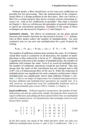
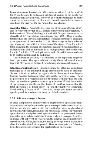
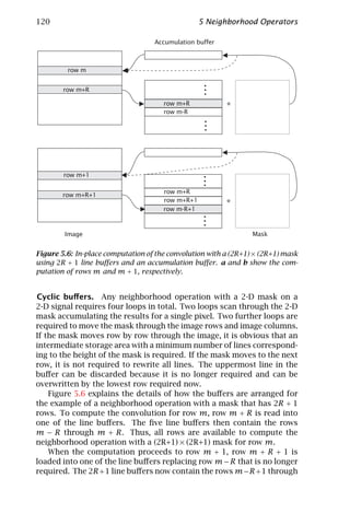
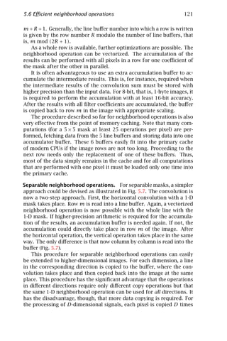
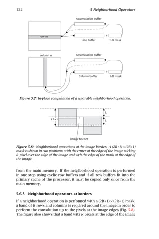
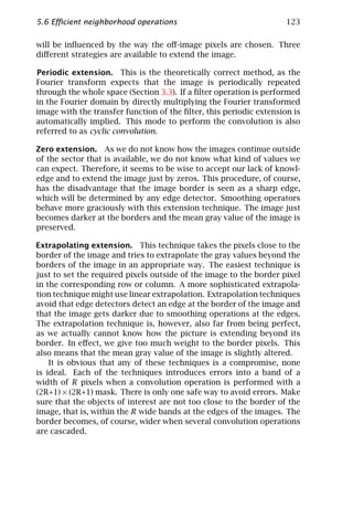
![124 5 Neighborhood Operators
5.7 References
[1] Jähne, B., (1997). Digital Image Processing—Concepts, Algorithms, and
Scientific Applications, 4th edition. New York: Springer.
[2] Zachmanoglou, E. C. and Thoe, D. W., (1986). Introduction to Partial Dif-
ferential Equations with Applications. New York: Dover Publications.
[3] Oppenheim, A. V. and Schafer, R. W., (1989). Discrete-time Signal Process-
ing. Prentice-Hall Signal Processing Series. Englewood Cliffs, NJ: Prentice-
Hall.
[4] Jähne, B., (1997). Handbook of Digital Image Processing for Scientific Ap-
plications. Boca Raton, FL: CRC Press.
[5] Lim, J. S., (1990). Two-dimensional Signal and Image Processing. Engle-
wood Cliffs, NJ: Prentice-Hall.
[6] Poularikas, A. D. (ed.), (1996). The Transforms and Applications Hand-
book. Boca Raton, FL: CRC Press.
[7] Pitas, I. and Venetsanopoulos, A. N., (1990). Nonlinear Digital Filters. Prin-
ciples and Applications. Norwell, MA: Kluwer Academic Publishers.
[8] Granlund, G. H. and Knutsson, H., (1995). Signal Processing for Computer
Vision. Norwell, MA: Kluwer Academic Publishers.
[9] Knutsson, H. and Westin, C.-F., (1993). Normalized and differential con-
volution. In Proceedings CVPR’93, New York City, NY, pp. 515–523, IEEE.
Washington, DC: IEEE Computer Society Press.
[10] Freeman, W. T. and Adelson, E. H., (1991). The design and use of steerable
filters. IEEE Transactions on Pattern Analysis and Machine Intelligence, 13:
891–906.
[11] Blahut, R., (1985). Fast Algorithms for Digital Signal Processing. Reading,
MA: Addison-Wesley.
[12] Selesnick, I. W. and Burrus, C. S., (1997). Fast convolution and filtering. In
The Digital Signal Processing Handbook, V. K. Madisetti and D. B. Williams,
eds.,. Boca Raton, FL: CRC Press.](https://image.slidesharecdn.com/computervision-handbookofcomputervisionandapplicationsvolume2-signalprocessingandpatternrecognition-120205081400-phpapp02/85/Computer-vision-handbook-of-computer-vision-and-applications-volume-2-signal-processing-and-pattern-recognition-149-320.jpg)
![6 Principles of Filter Design
Bernd Jähne, Hanno Scharr, and Stefan Körkel
Interdisziplinäres Zentrum für Wissenschaftliches Rechnen (IWR)
Universität Heidelberg, Germany
6.1 Introduction . . . . . . . . . . . . . . . . . . . . . . . . . . . . . . . . 125
6.2 Filter design criteria . . . . . . . . . . . . . . . . . . . . . . . . . . . 126
6.2.1 Classical design criteria in signal processing . . . . . . 126
6.2.2 Filter design criteria for computer vision . . . . . . . . 127
6.3 Windowing techniques . . . . . . . . . . . . . . . . . . . . . . . . . 128
6.4 Filter cascading . . . . . . . . . . . . . . . . . . . . . . . . . . . . . . 132
6.5 Filter design as an optimization problem . . . . . . . . . . . . . 133
6.5.1 Parameterized ansatz . . . . . . . . . . . . . . . . . . . . . 134
6.5.2 Reference function . . . . . . . . . . . . . . . . . . . . . . . 136
6.5.3 Error functional . . . . . . . . . . . . . . . . . . . . . . . . 137
6.5.4 Solution strategies . . . . . . . . . . . . . . . . . . . . . . . 138
6.5.5 Examples . . . . . . . . . . . . . . . . . . . . . . . . . . . . . 139
6.6 Design of steerable filters and filter families . . . . . . . . . . . 143
6.6.1 Gradient computation . . . . . . . . . . . . . . . . . . . . 144
6.6.2 Steerable one-dimensional higher-order derivatives . 145
6.6.3 Optimization of filter families . . . . . . . . . . . . . . . 145
6.7 References . . . . . . . . . . . . . . . . . . . . . . . . . . . . . . . . . 151
6.1 Introduction
Filter design is a well-established area both in continuous-time and
discrete-time signal processing and subject of standard textbooks [1, 2].
This is not the case, however, for multidimensional signal processing
for three reasons:
• Filter design of higher-dimensional signals poses difficult mathe-
matical problems [3, Chapter 2].
• While design criteria for the analysis of 1-D signals (time series)
are quite clear, this is less certain for higher-dimensional signals
including images.
125
Handbook of Computer Vision and Applications Copyright © 1999 by Academic Press
Volume 2 All rights of reproduction in any form reserved.
Signal Processing and Pattern Recognition ISBN 0–12–379772-1/$30.00](https://image.slidesharecdn.com/computervision-handbookofcomputervisionandapplicationsvolume2-signalprocessingandpatternrecognition-120205081400-phpapp02/85/Computer-vision-handbook-of-computer-vision-and-applications-volume-2-signal-processing-and-pattern-recognition-150-320.jpg)
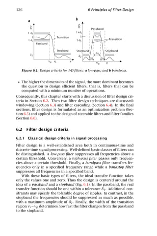
![6.2 Filter design criteria 127
1
0.8
0.6
0.4
0.2
0
-0.2
-20 -10 0 10 n 20
Figure 6.2: Disadvantage of classical 1-D filtering for computer vision: convo-
lution of a step edge with an ideal low-pass filter causes overshoots.
An ideal filter, that is, a filter with a flat passband and stopband
and a zero width transition region, can only be realized by a mask with
an infinite number of coefficients. This general rule is caused by the
reciprocity between the Fourier and space domains (Section 3.2.3). A
discontinuity as shown for the ideal low-pass filter in Fig. 6.1a causes
the envelope of the filter coefficients to decrease not faster than with
1/x from the center coefficient. From the uncertainty relation (Sec-
tion 3.2.3), we can conclude that the narrower the selected wave-number
range of a filter is, the larger its filter mask is.
Discrete-time signal processing is dominated by causal recursive
filters (Section 5.4). This type of filters is more efficient than finite
impulse response filters, that is, less filter coefficients are required to
meet the same design criteria.
Filter design of 1-D filters according to the criteria discussed here
is treated extensively in standard textbooks of signal processing. Good
examples are, for example, [1, Chapter 7] and [2, Chapter 8].
6.2.2 Filter design criteria for computer vision
These design criteria for 1-D signals can, in principle, be applied for
higher-dimensional signals including images. Depending on the appli-
cation, the shape of the passband and/or stopband could be either cir-
cular (hyperspherical) for isotropic filters or rectangular (hypercubic)
for separable filters. However, it is not advisable to use filters designed
for the analysis of time series blindly in computer vision.
We demonstrate the disadvantages of these criteria applied to im-
ages with an ideal low-pass filter. Figure 6.2 shows that filtering of a
step edge with an ideal low-pass filter leads to undesirable overshoot-
ing effects including negative gray values. A causal recursive filter—
commonly used for time series—causes the edge to shift by a distance
proportional to the relaxation length of the filter.
Because both of these effects are undesirable for computer vision,
different design criteria have to be applied for filters to be used for](https://image.slidesharecdn.com/computervision-handbookofcomputervisionandapplicationsvolume2-signalprocessingandpatternrecognition-120205081400-phpapp02/85/Computer-vision-handbook-of-computer-vision-and-applications-volume-2-signal-processing-and-pattern-recognition-152-320.jpg)
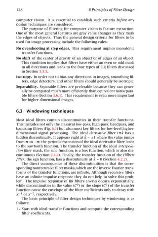
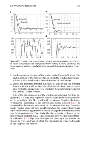
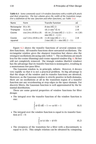
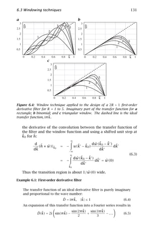
![132 6 Principles of Filter Design
corresponding to the following odd filter mask with the coefficients
(−1)r
hr = −h−r = r ∈ [1, R] (6.6)
r
The usage of the rectangular window would be equivalent to keeping
only a number of elements in the Fourier series. As Fig. 6.4a shows, the
oscillations are still large and the slope of the transfer function at low
wave numbers flips with the order of the series between 0 and twice
the correct value. Thus, the resulting truncated filter is not useful at
all.
Much better results can be gained by using a binomial window func-
tion.
Window Resulting mask
1/4[1 2 1] 1/2[1 0 –1]
(6.7)
1/16[1 4 6 4 1] 1/12[–1 8 0 –8 1]
1/64[1 6 15 20 15 6 1] 1/60[1 –9 45 0 –45 9 –1]
These approximations show no oscillations; the deviation from the
ideal response increases monotonically (Fig. 6.4b). The convergence,
however, is quite slow. Even a filter with 11 coefficients (R = 5) shows
significant deviations from the ideal transfer functions for wave num-
˜
bers k > 0.6.
A triangular window results in other deficits (Fig. 6.4c). Although
the transfer function is close to the ideal transfer function for much
higher wave numbers, the slope of the transfer function is generally
too low.
Example 6.1 indicates some general weaknesses of the windowing
technique for filter design. While it is quite useful for filters with flat
responses and discontinuities such as ideal low-pass filters in balancing
overshooting and ripples vs steepness of the transitions, it does not
obviously lead to optimal solutions. It is not clear in which way the
filters are improved by the different windows.
6.4 Filter cascading
Cascading of simple filters is a valuable approach to filter design, es-
pecially for higher-dimensional signals. Complex filters can be built
by applying simple 1-D filters repeatedly in all directions of the signal.
This approach has a number of significant advantages.
Known properties. The properties of the simple filters are well known.
The transfer function can be expressed analytically in simple equa-
tions. As cascading of filters simply means the multiplication of the
transfer functions, the resulting transfer functions for even complex
filters can be computed easily and analyzed analytically.](https://image.slidesharecdn.com/computervision-handbookofcomputervisionandapplicationsvolume2-signalprocessingandpatternrecognition-120205081400-phpapp02/85/Computer-vision-handbook-of-computer-vision-and-applications-volume-2-signal-processing-and-pattern-recognition-157-320.jpg)
![6.5 Filter design as an optimization problem 135
This constraint is used to set the value of the first coefficient d1 to
R
d1 = 1/2 − dr r (6.11)
r =2
If we introduce this equation into Eq. (6.9), we obtain a new con-
strained ansatz function with only R − 1 parameters:
R
ˆ ˜ ˜
D(k) = i sin(π k) + 2i ˜ ˜
dr (sin(π r k) − r sin(π k)) (6.12)
r =2
If a recursive filter is included into the first-order derivative filter, the
ansatz function becomes nonlinear in the filter coefficients for the
recursive part of the filter. The simplest case is the inclusion of the
relaxation filter running back and forth as discussed in Section 5.4.6,
Eq. (5.55). This filter adds one more parameter d0 and the ansatz
function becomes
R
˜
(1 − d0 )2 i sin(π k) + 2i ˜ ˜
dr (sin(π r k) − r sin(π k))
r =2
ˆ ˜
D(k) =
˜
1 + d2 − 2d0 cos(π k)
0
(6.13)
Example 6.3: Smoothing filter
A normalized even smoothing filter with a 2R + 1 mask
[bR , . . . , b1 , b0 , b1 , . . . , bR ] (6.14)
meets the constraint that the sum of all coefficients is equal to one.
This can be forced by
R
b0 = 1 − 2 br (6.15)
r =1
ˆ
The resulting transfer function B can then be written as
R
ˆ ˜
B(k) = 1 + 2 ˜
br (cos(r π k) − 1) (6.16)
r =1
Example 6.4: Hilbert filter
A Hilbert filter (Section 4.2.2) is also of odd symmetry. Thus it has the
same ansatz function as a first-order derivative filter in Eq. (6.9). The
constraint applied in Eq. (6.12), however, makes no sense for a Hilbert
filter. It may be useful to add the constraint that the Hilbert filter
˜
is symmetrical around k = 0.5. This additional symmetry constraint](https://image.slidesharecdn.com/computervision-handbookofcomputervisionandapplicationsvolume2-signalprocessingandpatternrecognition-120205081400-phpapp02/85/Computer-vision-handbook-of-computer-vision-and-applications-volume-2-signal-processing-and-pattern-recognition-160-320.jpg)
![136 6 Principles of Filter Design
forces all filter coefficients with even r in Eq. (6.9) to zero. Thus the
ansatz function for such a symmetric Hilbert filter is
R
ˆ ˜
D(k) = 2i ˜
d2r −1 sin(π (2r − 1)k) (6.17)
r =1
As with the first-order derivative filter, a recursive part can be included
into the design of a Hilbert filter. As the correction that is performed
˜
by such a recursive filter must also be symmetric around k = 0.5 (H(1−ˆ
˜ = H(k)) and enhance lower and higher wave numbers, the following
k) ˆ ˜
ansatz function is useful:
R
ˆ ˜ (1 + d0 )2 ˜
H(k) = 2i d2r −1 sin(π (2r − 1)k) (6.18)
˜
1 + d2 − 2d0 cos(2π k)
0 r =1
The recursive filter is a mirrored relaxation filter (Section 5.4.6) with
double step width.
6.5.2 Reference function
At first glance, it appears that not much has to be said about the ref-
erence function because often it is simply the ideal transfer function.
This is, however, not always the best choice. As an example, we discuss
the reference function for a first-order derivative filter in multidimen-
sional signals.
Example 6.5: First-order derivative filter
The transfer function of an ideal first-order derivative filter in the
direction d is
ˆ ˜ ˜
Dd (k) = iπ kd (6.19)
This is not always the best choice as a reference function as it is of-
ten required that only the gradient direction, for example, for motion
determination in spatiotemporal images (Chapter 13), must be cor-
rect. The direction of the gradient can be expressed by the angles
of polar coordinates in a natural way. The angles φi occurring in D-
dimensional polar coordinates for the gradient direction are
φ1 = ˜ ˜
arctan k2 /k1 ∈ ] − π, π]
1/2
˜
d
(6.20)
φd = arctan kd+1 ˜
k2 ∈ [−π /2, π /2]
d
d =1
ˆ ˜ ˜
as the ideal transfer function of the derivative is D0 (k) = iπ k. Fig-
ure 6.5 explains the square root term in the denominator of the pre-
ceding formula for higher dimensions. Thus this set of angles is now
the reference function and has to be compared with the angles of the
gradient computed by the filter.](https://image.slidesharecdn.com/computervision-handbookofcomputervisionandapplicationsvolume2-signalprocessingandpatternrecognition-120205081400-phpapp02/85/Computer-vision-handbook-of-computer-vision-and-applications-volume-2-signal-processing-and-pattern-recognition-161-320.jpg)
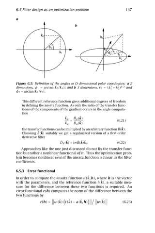
![6.5 Filter design as an optimization problem 139
This optimization problem is (generally) a nonlinear regression prob-
lem. Problems of this type can be solved by a generalized Gauss-
Newton-method, for example, [4, Section 6.1] .
Maximum norm. Using the maximum norm (L∞ ), the Eq. (6.26) is not
differentiable. Therefore we reformulate the problem using an addi-
tional variable δ
δ := max ˜
d(kj , h) (6.28)
j =1,... ,J
and write the maximum of the absolute value in Eq. (6.28) as inequality
constraints
˜
−δ ≤ d(kj , h) ≤ δ ∀ j = 1, . . . , J
We obtain the following inequality constrained (generally) nonlinear op-
timization problem
˜
min δ, subject to − δ ≤ d(kj , h) ≤ δ ∀ j = 1, . . . , J (6.29)
δ,h
Such problems can be solved by a successive quadratic programming
(SQP) method, for example, [5, Chapter 6] or [4, Section 12.4].
Fixed-point optimization. Using the methods described here, we get
real numbers for the optimal filter coefficients. Because of recent hard-
ware developments (like Intel’s MMX or Sun’s VIS) that improve integer
arithmetic performance in computational calculations, it is also desir-
able to optimize filters with integer or rational filter coefficients.
Therefore we formulate the forementioned optimization problems
as nonlinear integer problem, more precisely, we discretize the coeffi-
cient variable space
hr = αr /2M , r = 1, . . . , R, αr ∈ Z
with M chosen suitably. We optimize over the integer variables αr in-
stead of hr . Problems of this type are known to be NP-hard [6, Section
I.5]. In our case we use the branch and bound method [7, Chapter 5.3,
Section 6.2] combined with the methods as described here for the solu-
tion of relaxed problems and some rounding heuristics to find integer
feasible solutions.
6.5.5 Examples
In this section, some examples illustrate the various optimization tech-
niques discussed in the previous sections.](https://image.slidesharecdn.com/computervision-handbookofcomputervisionandapplicationsvolume2-signalprocessingandpatternrecognition-120205081400-phpapp02/85/Computer-vision-handbook-of-computer-vision-and-applications-volume-2-signal-processing-and-pattern-recognition-164-320.jpg)
![140 6 Principles of Filter Design
a b
Figure 6.6: Error in transfer function of optimized 1-D first-order derivative
filters. Shown is the absolute deviation from the ideal transfer function iπ k ˜
for a nonrecursive filter according to Eq. (6.12) with two free parameters (solid
line floating-point solution, narrow-dashed line [28 -9 2]/32 integer coefficients,
and wide-dashed line [108 -31 6]/128 integer coefficients); and b recursive filter
according to Eq. (6.33) with two free parameters.
Table 6.2: Filter coefficients of first-order derivative filters optimized according
to Eq. (6.12) with 2R + 1 coefficients. The second column contains the filter
coefficients d1 , . . . , dR and the lower part of the table the coefficients for fixed-
point arithmetic with varying computational accuracy. Boldface filters are an
optimal choice with minimal filter coefficients and still an acceptable error as
compared to the floating-point solution.
R Filter coefficients Error
1 0.5 1.5 × 10⁻¹
2 0.758, -0.129 3.6 × 10⁻²
3 0.848, -0.246, 0.0480 1.3 × 10⁻²
4 0.896, -0.315, 0.107, -0.0215 5.6 × 10⁻³
5 0.924, -0.360, 0.152, -0.0533, 0.0109 2.8 × 10⁻³
6 0.942, -0.391, 0.187, -0.0827, 0.0293, -0.00601 1.6 × 10⁻³
2 [6, -1]/8 3.60 × 10⁻²
2 [12, -2]/16 3.60 × 10⁻²
2 [24, -4]/32 3.60 × 10⁻²
2 [48, -8]/64 3.60 × 10⁻²
2 [96, -16]/128 3.60 × 10⁻²
2 [194, -33]/256 3.57 × 10⁻²
3 [6, -1, 0]/8 3.6 × 10⁻²
3 [12, -2, 0]/16 3.6 × 10⁻²
3 [28, -9, 2]/32 1.6 × 10⁻²
3 [55, -16, 3]/64 1.5 × 10⁻²
3 [108, -31, 6]/128 1.3 × 10⁻²
3 [216, -62, 12]/256 1.3 × 10−2](https://image.slidesharecdn.com/computervision-handbookofcomputervisionandapplicationsvolume2-signalprocessingandpatternrecognition-120205081400-phpapp02/85/Computer-vision-handbook-of-computer-vision-and-applications-volume-2-signal-processing-and-pattern-recognition-165-320.jpg)
![6.5 Filter design as an optimization problem 141
Example 6.6: Optimal 1-D first-order derivative filter
The classical approaches to optimized 1-D derivative filters are well
described in standard textbooks [8, 9]. For the optimization of a 1-D
first-order derivative filter, the transfer function of the ideal derivative
filter (Eq. (6.19)) is directly taken as the reference function.
Finite impulse response ansatz function. In this case, we take the
ansatz function Eq. (6.12) with the additional constraint that we force
the slope of the transfer function for small wave numbers to be i π k. ˜
Equation (6.12) is valid for filters with an odd number of coefficients
(2R + 1) with the mask
D = [dR , . . . , d1 , 0, −d1 , . . . , −dR ] (6.30)
For even-length filters the mask is
D = [dR , . . . , d1 , −d1 , . . . , −dR ] (6.31)
and the ansatz function is slightly different from Eq. (6.12):
R
ˆ ˜ ˜
D(k) = i sin(π k/2) + 2i ˜ ˜
dr (sin(π (r − 1/2)k) − (r − 1/2) sin(π k))
r =2
(6.32)
Infinite impulse response ansatz function. The ansatz function in
Eq. (6.13) can be taken for optimization of filters with real filter coef-
ficients for floating-point arithmetic. In integer arithmetic we directly
include the coefficent α1 /2M of the recursive relaxation filter:
ˆ ˜ (1 − α1 /2M )2
D(k) = i
1 + α2 /22M ˜
− 2(α1 /2M ) cos(π k)
1
(6.33)
R
˜
sin(π k) + 2 αr ˜
/2M (sin(π r k) − r ˜
sin(π k))
r =2
The filter coefficients shown in Tables 6.2 and 6.3 and the correspond-
ing transfer functions depicted in Fig. 6.6 are computed using the L2
˜ ˜
norm combined with the weighting function w(k) = cos4 (π k/2).
Example 6.7: Optimal Hilbert filter
As an example for the influence of the weighting function we use the
1-D Hilbert filter. As it is separable in n-D, the solution is valid for
higher dimensions, too.
ˆ
Reference function. We choose the transfer function Hr of the ideal
Hilbert filter as reference function:
ˆ ˜
Hr (k) = i sgn(k)
Ansatz function. For weighting functions with a symmetry of around
˜
k = 0.5 we use the ansatz function Eq. (6.17). If the weighting func-
tion does not have this symmetry, the optimal filter will not have it](https://image.slidesharecdn.com/computervision-handbookofcomputervisionandapplicationsvolume2-signalprocessingandpatternrecognition-120205081400-phpapp02/85/Computer-vision-handbook-of-computer-vision-and-applications-volume-2-signal-processing-and-pattern-recognition-166-320.jpg)
![142 6 Principles of Filter Design
Table 6.3: Filter coefficients of first-order derivative filters optimized accord-
ing to Eq. (6.33) with 2R + 1 coefficients; the second column contains the filter
coefficients d0 , d1 , . . . , dR , where d0 is the filter coefficient for the recursive re-
laxation filter part, and the lower part of the table the coefficients for fixed-point
arithmetic (note the loss of coefficients for small denominators shown for R = 5).
R Filter coefficients Error
1 -3.13, 0.5 1.1 × 10⁻²
2 -0.483, 0.442, 0.0292 2.1 × 10⁻³
3 -0.583, 0.415, 0.0487, -0.00427 6.4 × 10⁻⁴
4 -0.650, 0.402, 0.0596, -0.00851, 0.00112 2.4 × 10⁻⁴
5 0.698, 0.394, 0.0662, -0.0115, 0.00249, -0.000400 1.1 × 10⁻⁴
1 [801, 128]/256 1.1 × 10⁻²
2 [-120, 114, 7]/256 2.3 × 10⁻³
3 [-146, 107, 12, -1]/256 6.8 × 10⁻⁴
4 [-146, 107, 12, -1, 0]/256 6.8 × 10⁻⁴
5 [-146, 107, 12, -1, 0, 0]/256 6.8 × 10⁻⁴
5 [-651, 414, 59, -8, 1, 0]/1024 2.8 × 10⁻⁴
5 [-1495, 799, 142, -26, 6, -1]/2048 2.0 × 10⁻²
either. In that case we choose a filter mask [hR · · · h1 0 −h1 · · · −hR ],
as the 1-D Hilbert filter shall be imaginary and antisymmetric. The
ˆ
corresponding transfer function H is
R
ˆ ˜
H(k, h) = 2 i ˜
hr sin(r π k) (6.34)
r =1
The filter coefficients are computed in L2 norm combined with a weight-
˜
ing function cos4 (π /2 k) and given in Table 6.4. The slow convergence
of the error indicates that the ansatz function with the weighting func-
˜
tion cos4 (π /2 k) was not chosen properly. It puts the most weight at
the discontinuity of the Hilbert filter at ˜ = 0 (the discontinuities at
(k)
˜ = ±1 are suppressed), which cannot be well approximated with a
(k)
series of sinusoidal functions.
˜
The weighting function sin2 (π k), which emphasizes wave numbers
˜ ˜
around k = 0.5 and a Hilbert filter that is even with respect to k = 0.5,
gives much better results (Table 6.5).](https://image.slidesharecdn.com/computervision-handbookofcomputervisionandapplicationsvolume2-signalprocessingandpatternrecognition-120205081400-phpapp02/85/Computer-vision-handbook-of-computer-vision-and-applications-volume-2-signal-processing-and-pattern-recognition-167-320.jpg)
![6.6 Design of steerable filters and filter families 143
Table 6.4: Filter coefficients of Hilbert filters optimized according to Eq. (6.34)
˜
with 2R + 1 coefficients and weighting function cos4 (π /2 k); the second column
contains the filter coefficients d1 , . . . , dR in floating point arithmetic.
R Filter coefficients Error
1 0.776 5.31 × 10⁻¹
2 0.274, 0.439 4.53 × 10⁻¹
3 0.922, –0.391, 0.467 3.89 × 10⁻¹
4 0.228, 0.651, 0.426, 0.409 3.54 × 10⁻¹
5 1.038, –0.671, 0.937, –0.560, 0.394 3.26 × 10⁻¹
Table 6.5: Filter coefficients of Hilbert filters optimized according to Eq. (6.17)
˜
with 4R − 1 coefficients and weighting function sin2 (π k); The corresponding
filter coefficients are given; the second column contains the filter coefficients
d1 , . . . , dR in floating point arithmetic and the lower part of the table the coef-
ficients for fixed-point arithmetic.
R Filter coefficients Error
1 0.543 1.3 × 10⁻¹
2 0.599, 0.111 4.4 × 10⁻²
3 0.616, 0.154, 0.0431 2.1 × 10⁻²
4 0.624, 0.175, 0.0698, 0.0214 1.2 × 10⁻²
5 0.627, 0.186, 0.0861, 0.0384, 0.0122 7.5 × 10⁻³
1 [139]/256 1.3 × 10⁻¹
2 [153, 28]/256 4.4 × 10⁻²
3 [158, 40, 11]/256 2.1 × 10⁻²
4 [160, 46, 19, 6]/256 1.2 × 10⁻²
5 [161, 48, 22, 10, 3]/256 8.0 × 10⁻³
6.6 Design of steerable filters and filter families
Steerable filters are well described in the literature [for example, 10, 11,
12, 13, 14, 15]. Because of existing detailed mathematical treatments
[see, for example, 16, 17], only a short introduction to steerability shall
be given here. As angular steerability is the most common case, it is
used as an explanatory example, but steerability in any other domain
works in the same way.
Steerable filters are a special case of filter families, fulfilling the sam-
pling theorem (see Section 2.4) exactly in a specific domain. Therefore,
the interpolation of the filter responses to a continuous response is
exactly possible.](https://image.slidesharecdn.com/computervision-handbookofcomputervisionandapplicationsvolume2-signalprocessingandpatternrecognition-120205081400-phpapp02/85/Computer-vision-handbook-of-computer-vision-and-applications-volume-2-signal-processing-and-pattern-recognition-168-320.jpg)
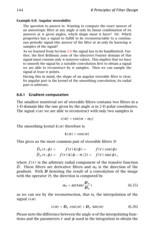
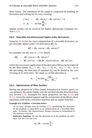
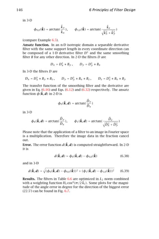
![6.6 Design of steerable filters and filter families 147
Table 6.6: Filter coefficients for derivative filters optimized according to either
Eq. (6.38) or Eq. (6.39). The first and second columns contain the filter parts. The
first part of the table lists well-known approaches, followed by optimal filters in
floating point and fixed-point arithmetic. The last part summarizes the results
of a study on varying the denominator for fixed-point arithmetic.
Derivative Smoothing Error Name
−4
(odd mask) (even mask) [10 ]
[1, 0]/2 none 400 3 tab
[1, 2, 0]/6 none 1700 5 tab.a
[-1, 8, 0]/12 none 150 5 tab.b
[1] [1]/2 180 2×2
[1, 0]/2 [1, 2]/4 190 Sobel
[-1, 8, 0]/12 [1, 4, 6]/16 800 5×5 Gauß
[-0.262, 1.525, 0 ] none 93 5-tab.opt
[1, 0]/2 [46.84 162.32]/256 22 3×3-opt
[77.68, 139.48]/256 [16.44, 111.56]/256 3.4 4×4-opt
[21.27, 85.46, 0]/256 [5.91, 61.77, 120.64]/256 0.67 5 ×5-opt
[21.38, 85.24, 0]/256 [5.96, 61.81, 120.46]/256 1.1 5×5×5-opt
[-67, 390 0]/256 none 92 5-tab.int
[1, 0]/2 [47, 162]/256 22 3×3-int
[76, 142]/256 [16, 112]/256 3.9 4×4-int
[24, 80, 0]/256 [7, 63, 116]/256 1.9 5×5-int
[1, 0]/2 [1, 2]/4 190 3×3-int
[1, 0]/2 [1, 6]/8 150 3×3-int
[1, 0]/2 [3, 10]/16 26 3×3-int
[1, 0]/2 [6, 20]/32 26 3 ×3-int
[1, 0]/2 [12, 40]/64 26 3×3-int
[1, 0]/2 [23, 82]/128 25 3×3-int
[1, 0]/2 [47, 162]/256 23.16 3×3-int
[1, 0]/2 [46.84, 162.32]/256 23.11 3×3-opt
Example 6.10: Gradient filters on a hexagonal grid
On a hexagonal grid only the ansatz function differs from the Carte-
sian case; reference function and error are the same. As in the Carte-
sian case there are two ways to get an ansatz function: a direct one
simply using the fact that we want to compute the derivative; and a
steerable one respecting the fact that we want to compute a direction.](https://image.slidesharecdn.com/computervision-handbookofcomputervisionandapplicationsvolume2-signalprocessingandpatternrecognition-120205081400-phpapp02/85/Computer-vision-handbook-of-computer-vision-and-applications-volume-2-signal-processing-and-pattern-recognition-172-320.jpg)
![148 6 Principles of Filter Design
a b c
14 14 3
12 12 2.5
10 10
2
8 8
1.5
6 6
1
4 4
2 2 0.5
0 0 0
0 0.1 0.2 0.3 0.4 0.5 0.6 0 0.1 0.2 0.3 0.4 0.5 0.6 0 0.1 0.2 0.3 0.4 0.5 0.6
d e f
14
18 0.0005
12 16
14 0.0004
10
12
8 0.0003
10
6 8
0.0002
6
4
4 0.0001
2 2
0 0
0 0 0.1 0.2 0.3 0.4 0.5 0.6 0 0.1 0.2 0.3 0.4 0.5 0.6
0 0.1 0.2 0.3 0.4 0.5 0.6
Figure 6.7: Magnitude of the angle error in degree for the direction of the
largest error (22.5°). Upper line: 3 × 3-filters (a symmetric difference, b Sobel,
c optimized). Lower line: 5 × 5-filters (d [-1 8 0 -8 1]/16, e derivative of Gauss,
f optimized; refer to results in Example 6.9 and Table 6.6). Please note the
different scales of the y axes.
Direct ansatz. A direct ansatz for the derivative filters is
d −d
1
Dx = 1−d 0 −(1 − d) (6.40)
2
d −d
−1 −1
1
Dy = √ 0 0 0 (6.41)
2 3
1 1
with the transfer functions
√
ˆ ˜ 3π ˜ π˜
Dx = (1 − d) sin(π kx ) + 2 d cos( ky ) sin( kx )
2 2
√
ˆ 2 3π ˜ π˜
Dy = √ sin( ky ) cos( kx )
3 2 2
For this size of filters there are no more degrees of freedom, consid-
ˆ ˜
ering the symmetries and the claim D(k = 0) = i . With these filters
the reference function and error can be computed in the same way as
in the 2-D case on a Cartesian grid.
Steerability ansatz. Gradient computation can be understood as com-
putation of the maximum of the response Dφ of a set of steerable](https://image.slidesharecdn.com/computervision-handbookofcomputervisionandapplicationsvolume2-signalprocessingandpatternrecognition-120205081400-phpapp02/85/Computer-vision-handbook-of-computer-vision-and-applications-volume-2-signal-processing-and-pattern-recognition-173-320.jpg)
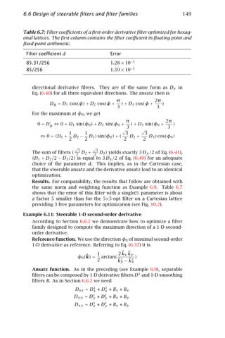
![150 6 Principles of Filter Design
Table 6.8: Filter coefficients di of the optimized second-order steerable deriva-
tive filter basis according to Eq. (6.42); the first column contains the filter coef-
ficients; the first part of the table lists well-known approaches, followed by the
optimal filters in floating point arithmetic.
Filter coefficients Error
1/12, 0, 0, -1/6 4.69 × 10⁻²
1/12, 4/16, 1/16, -1/6 3.72 × 10⁻²
0.208, 0.113, -0.137, 0.128 2.54 × 10⁻⁴
where the symbols for the filters do not always denote the same filter
but the same filter behavior. For example, a 5 × 5 filter family is
Dxx = [1 − 1]x ∗ [1 − 1]x ∗ [d0 (1 − 2 d0 ) d0 ]x ∗
[d2 d1 (1 − 2(d1 + d2 )) d1 d2 ]y ,
Dyy = [1 − 1]y ∗ [1 − 1]y ∗ [d0 (1 − 2 d0 ) d0 ]y ∗
(6.42)
[d2 d1 (1 − 2(d1 + d2 )) d1 d2 ]x ,
1
Dxy = 4 [d3 (1 − 2d3 ) 0 − (1 − 2d3 ) − d3 ]x ∗
[d3 (1 − 2d3 ) 0 − (1 − 2d3 ) − d3 ]y
For this filter family all symmetries and degrees of freedom d are
already considered. Standard parameter choices are
d0 = 1/12, d1 = d2 = 0, d3 = −1/6
and
d0 = 1/12, d1 = 4/16, d2 = 1/16, d3 = −1/6
˜
where the occurring derivative filters are optimized for small k and
there is either no or Gaussian smoothing in cross direction.
The ansatz function φ is
1 ˆ
2 Dxy
˜
φ(k, d) = arctan( )
2 ˆ yy − Dxx
D ˆ
The transfer function of the smoothing filters B and the derivatives d
are given in Eq. (6.16) and Eqs. (6.12) and (6.32), respectively.
Results. For the example filter family of Eq. (6.42) the parameters d
are given in Table 6.8. All results are computed in L2 norm combined
˜
with the weighting function Πi cos(π /2 ki )4 .](https://image.slidesharecdn.com/computervision-handbookofcomputervisionandapplicationsvolume2-signalprocessingandpatternrecognition-120205081400-phpapp02/85/Computer-vision-handbook-of-computer-vision-and-applications-volume-2-signal-processing-and-pattern-recognition-175-320.jpg)
![6.7 References 151
6.7 References
[1] Oppenheim, (1975). Digital signal processing. Englewood Cliffs, NJ:
Pentice-Hall.
[2] Proakis, J. G. and Manolakis, D. G., (1992). Digital Signal Processing. Prin-
ciples, Algorithms, and Applications. New York: McMillan.
[3] Lim, J. S., (1990). Two-dimensional Signal and Image Processing. Engle-
wood Cliffs, NJ: Prentice-Hall.
[4] Fletcher, R., (1987). Practical Methods of Optimization, 2 edition. New
York: Wiley.
[5] Gill, P., Murray, W., and Wright, M., (1981). Practical Optimization. London:
Academic Press.
[6] Nemhauser, G. and Wolsey, L., (1988). Integer and Combinatorial Opti-
mization. New York: J. Wiley.
[7] Floudas, C., (1995). Nonlinear and Mixed-Integer Optimization. Oxford:
Oxford University Press.
[8] Oppenheim, A. V. and Schafer, R. W., (1989). Discrete-Time Signal Process-
ing. Englewood Cliffs, NJ: Prentice Hall.
[9] Proakis, J. G. and Manolakis, D. G., (1992). Digital Signal Processing, Prin-
ciples, Algorithms, and Applications. New York: Macmillan.
[10] Karasaridis, A. and Simoncelli, E. P., (1996). A filter design technique for
steerable pyramid image transforms. In ICASSP, Vol. IV, pp. 2389–2392.
Atlanta, GA: IEEE Sig. Proc. Society.
[11] Manduchi, R. and Perona, P., (1995). Pyramidal implementation of de-
formable kernels. In Proc. International Conference on Image Processing,
pp. 378–381. Washington: IEEE.
[12] Perona, P., (1991). Deformable kernels for early vision. Technical Report
MIT-LIDS-P-2039, California Institute of Technology 116-81, Pasadena. CA
91126, USA.
[13] Perona, P., (1992). Steerable-scalable kernels for edge detection and junc-
tion analysis. Image and Vision Comp., 10:663–672.
[14] Simoncelli, E. and Farid, H., (1996). Steerable Wedge Filters for Local Ori-
entation Analysis. IEEE Trans Image Proc, 5(9):1377–1382.
[15] Simoncelli, E. P., Freeman, W. T., Adelson, E. H., and Heeger, D. J., (1992).
Shiftable multiscale transforms. IEEE Trans. Information Theory, 38:587–
607.
[16] Manduchi, R., Perona, P., and Shy, D., (1997). Efficient implementation
of deformable filter banks. Technical Report CNS-TR-97-04, California
Institute of Technology 116-81, Pasadena. CA 91126, USA.
[17] Freeman, W. T. and Adelson, E. H., (1991). The design and use of steerable
filters. IEEE Trans. Patt. Anal. Mach. Intell., 13:891–906.](https://image.slidesharecdn.com/computervision-handbookofcomputervisionandapplicationsvolume2-signalprocessingandpatternrecognition-120205081400-phpapp02/85/Computer-vision-handbook-of-computer-vision-and-applications-volume-2-signal-processing-and-pattern-recognition-176-320.jpg)

![154 7 Local Averaging
lattices. The discussion is not restricted to 2-D signals. Whenever it is
possible, the equations and filters are given for signals with arbitrary
dimension.
The common properties and characteristics of all averaging filters
are discussed in Section 7.2. On lattices two types of averaging filters
are possible [1, Sect. 5.7.3]. Type I filters generate an output on the
same lattice. On a rectangular grid such filters are of odd length in
all directions. Type II filters generate an output on a grid with lattice
points in-between the original lattice points (intermediate lattice). On a
rectangular grid such filters are of even length in all directions. In this
chapter two elementary averaging filters for digital multidimensional
signals are discussed, box filters (Section 7.3) and binomial filters (Sec-
tion 7.4). Then we will deal with techniques to cascade these elemen-
tary filters to large-scale averaging filters in Section 7.5. Filters with
weighted signals (normalized convolution) in Section 7.6.
7.2 Basic features
7.2.1 General properties of transfer functions
Any averaging filter operator must preserve the mean value. This con-
dition says that the transfer function for zero wave number is 1 or,
equivalently, that the sum of all coefficients of the mask is 1:
∞
ˆ
h(0) = 1 ⇐⇒ h(x) dDx = 1 or Hn = 1 (7.1)
−∞ n∈mask
Intuitively, we expect that any smoothing operator attenuates small-
er scales more strongly than coarser scales. More specifically, a smooth-
ing operator should not completely annul a certain scale while smaller
scales still remain in the image. Mathematically speaking, this means
that the transfer function decreases monotonically with the wave num-
ber. Then for any direction, represented by a unit vector r¯
ˆ ¯ ˆ ¯
h(k2 r ) ≤ h(k1 r ) if k2 > k1 (7.2)
We may impose the more stringent condition that the transfer func-
tion approaches zero in all directions,
ˆ r
lim h(k¯) = 0 (7.3)
k→∞
On a discrete lattice the wave numbers are limited by the Nyquist con-
dition, that is, the wave number must lay within the first Brillouin zone
(Section 2.4.2). Then it makes sense to demand that the transfer func-
tion of an averaging filter is zero at the border of the Brillouin zone.](https://image.slidesharecdn.com/computervision-handbookofcomputervisionandapplicationsvolume2-signalprocessingandpatternrecognition-120205081400-phpapp02/85/Computer-vision-handbook-of-computer-vision-and-applications-volume-2-signal-processing-and-pattern-recognition-179-320.jpg)
![7.2 Basic features 155
On a rectangular lattice this means
ˆ
h(k) = 0 if ˆ ˆ
kbd = |bd |/2 (7.4)
ˆ
where bd is any of the D-basis vectors of the reciprocal lattice (Sec-
tion 2.4.2). Together with the monotonicity condition and the preserva-
tion of the mean value, this means that the transfer function decreases
monotonically from one to zero for each averaging operator.
For a 1-D filter we can easily use Eq. (5.24) to relate the condition in
Eq. (7.4) to a condition for the coefficients of type I filters:
ˆ
h(1) = 0 ⇐ h0 + 2
⇒ hr = 2 hr (7.5)
r even r odd
One-dimensional type II filters are, according to Eq. (5.24), always zero
˜
for k = 1.
7.2.2 Symmetry and isotropy
Even filters in continuous space. With respect to object detection,
the most important feature of an averaging operator is that it must not
shift the object position. Any shift introduced by a preprocessing op-
erator would cause errors in the estimates of the position and possibly
other geometric features of an object. In order not to cause a spatial
shift, a filter must not induce any phase shift in the Fourier space. A
filter with this property is known as a zero-phase filter . This implies
that the transfer function is real and this is equivalent with an even
symmetry of the filter mask (Section 3.2.3):
⇒ˆ
h(−x) = h(x) ⇐ h(k) real (7.6)
Averaging filters normally meet a stronger symmetry condition in the
sense that each axis is a symmetry axis. Then Eq. (7.6) is valid for each
component of x:
h([x1 , . . . , −xd , . . . , xD ]T ) = h([x1 , . . . , xd , . . . , xD ]T ) (7.7)
Even filters on 1-D lattices. For digital signals we distinguish fil-
ters with odd and even numbers of coefficients in all directions (Sec-
tion 5.3.5). For both cases, we can write the symmetry condition for a
filter with Rd + 1 coefficients in the direction d as
Hr0 ,r1 ,... ,Rd −rd ,... ,rD = Hr0 ,r1 ,... ,rd ,... ,rD ∀d ∈ [1, D] (7.8)
when we count the coefficients in each direction from left to right from
0 to Rd . This is not the usual counting but it is convenient as only one
equation is required to express the evenness for filters with even and](https://image.slidesharecdn.com/computervision-handbookofcomputervisionandapplicationsvolume2-signalprocessingandpatternrecognition-120205081400-phpapp02/85/Computer-vision-handbook-of-computer-vision-and-applications-volume-2-signal-processing-and-pattern-recognition-180-320.jpg)
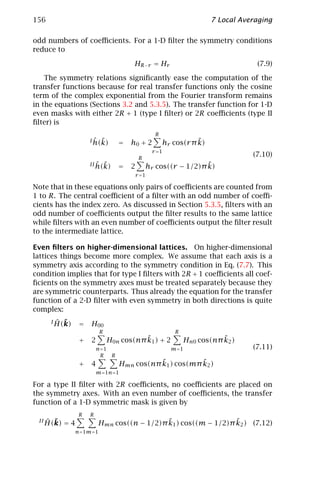
![7.2 Basic features 157
A further discussion of the properties of symmetric filters up to three
dimensions can be found in Jähne [2].
Isotropic filters. In most applications, the averaging should be the
same in all directions in order not to prefer any direction. Thus, both
the filter mask and the transfer function should be isotropic. Conse-
quently, the filter mask depends only on the magnitude of the distance
from the center pixel and the transfer function on the magnitude of the
wave number:
⇒ ˆ ˜ ˆ ˜
H(x) = H(|x |) ⇐ H(k) = H(|k|) (7.13)
This condition can also be met easily in discrete space. It means that
the coefficients at lattice points with an equal distance from the center
point are the same. However, the big difference now is that a filter
whose coefficients meet this condition has not necessarily an isotropic
transfer function. The deviations from the isotropy are stronger the
smaller the filter mask is. We will discuss the deviations from isotropy
in detail for specific filters.
7.2.3 Separable averaging filters
The importance of separable filters for higher-dimensional signals is
related to the fact that they can be computed much faster than non-
separable filters (Section 5.6.1). The symmetry conditions for separa-
ble averaging filters are also quite simple because only the symmetry
condition Eq. (7.9) must be considered. Likewise, the equations for the
transfer functions of separable filters are quite simple. If we apply the
same 1-D filter in all directions, the resulting transfer function of a
D-dimensional filter is given after Eq. (7.10) by
D R
ˆ ˜
I h(k) = h0 + 2 ˜
hr cos(r π kd )
d =1 r =1
D R
(7.14)
ˆ ˜
II h(k) = 2 ˜
hr cos((r − 1/2)π kd )
d =1 r =1
With respect to isotropy, there exists only a single separable filter
that is also isotropic, the Gaussian function
D
1 1 2
exp(−π x Tx/a2 ) = exp(−π xd /a2 ) ⇐⇒
aD aD
d =1
D
(7.15)
T
˜
exp(−π a2 k ˜
k/4) = ˜
exp(−π a2 k2 /4)
d
d =1](https://image.slidesharecdn.com/computervision-handbookofcomputervisionandapplicationsvolume2-signalprocessingandpatternrecognition-120205081400-phpapp02/85/Computer-vision-handbook-of-computer-vision-and-applications-volume-2-signal-processing-and-pattern-recognition-182-320.jpg)
![158 7 Local Averaging
a b
3
15 7
3
15 7
~ ~
k k
Figure 7.1: Transfer functions of type I box filters with 3, 7, and 15 coefficients
in a a linear plot; and b a log-log plot of the absolute value.
This feature shows the central importance of the Gaussian function for
signal processing from yet another perspective.
To a good approximation, the Gaussian function can be replaced
on orthogonal discrete lattices by the binomial distribution. The coef-
ficients of a 1-D binomal filter with R + 1 coefficients and its transfer
function are given by
1 R
BR = b0 = 1, . . . , br = ⇒ˆ ˜ ˜
, . . . , bR+1 = 1 ⇐ B R (k) = cosR (π k/2)
2R r
(7.16)
With the comments on the isotropy of discrete filters in mind (Sec-
tion 7.2.2), it is necessary to study the deviation of the transfer function
of binomial filters from an isotropic filter.
7.3 Box filters
The simplest method is to average pixels within the filter mask and to
divide the sum by the number of pixels. Such a simple filter is called
a box filter . It is also known under the name running mean. In this
section, type I (Section 7.3.1) and type II (Section 7.3.2) box filters and
box filters on hexagonal lattices (Section 7.3.3) are discussed.
7.3.1 Type I box filters
The simplest type I 1-D box filter is
1 1 2
3
R= ⇒ ˆ ˜ ˜
[1, 1, 1] ⇐ 3 R(k) = + cos(π k) (7.17)
3 3 3
The factor 1/3 scales the result of the convolution sum in order to
preserve the mean value (see Eq. (7.1) in Section 7.2.1). Generally, a](https://image.slidesharecdn.com/computervision-handbookofcomputervisionandapplicationsvolume2-signalprocessingandpatternrecognition-120205081400-phpapp02/85/Computer-vision-handbook-of-computer-vision-and-applications-volume-2-signal-processing-and-pattern-recognition-183-320.jpg)
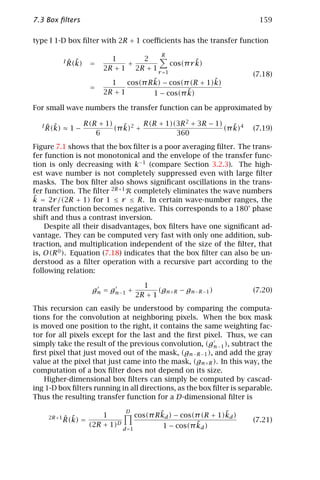
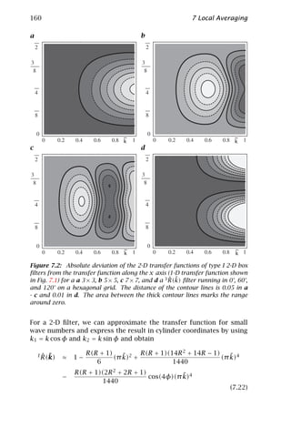
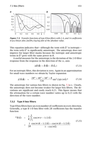
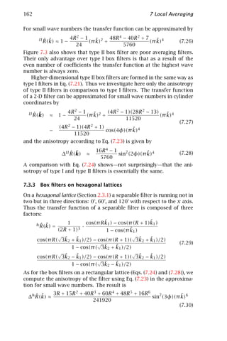
![7.4 Binomial filters 163
a b
2
16 4
32 8
2
4
32 16 8
~ ~
k k
Figure 7.4: Transfer functions of binomial filters BR in a a linear plot and b a
log-log plot of the absolute value with values of R as indicated.
This equation indicates that the effects of anisotropy are significantly
lower on hexagonal grids. In contrast to the box filters on a square grid,
˜ ˜
there is only an anisotropic term with k6 and not already with k4 . From
Fig. 7.2a and d we can conclude that the anisotropy is about a factor of
5 lower for a 3 R filter on a hexagonal lattice than on a square lattice.
7.4 Binomial filters
7.4.1 General properties
In Section 7.2.3 we concluded that only the Gaussian function meets the
most desirable features of an averaging filter: separability and isotropy.
In this section we will investigate to which extent the binomial filter,
which is a discrete approximation to the Gaussian filter, still meets
these criteria. The coefficients of the one-dimensional binomial filter
can be generated by repeatedly convolving the simple 1/2 [1 1] mask:
BR = 1/2 [1 1] ∗ . . . ∗ 1/2 [1 1] (7.31)
R times
This cascaded convolution is equivalent to the scheme in Pascal’s tri-
angle. The transfer function of the elementary B = 1/2 [1 1] filter is
ˆ ˜
B = cos(π k/2) (7.32)
There is no need to distinguish type I and type II binomial filters in the
equations because they can be generated by cascaded convolution as
in Eq. (7.31). Therefore, the transfer function of the BR binomial filter
is
R
ˆ ˜
B = cosR (π k/2) (7.33)
The most important features of binomial averaging filters are:](https://image.slidesharecdn.com/computervision-handbookofcomputervisionandapplicationsvolume2-signalprocessingandpatternrecognition-120205081400-phpapp02/85/Computer-vision-handbook-of-computer-vision-and-applications-volume-2-signal-processing-and-pattern-recognition-188-320.jpg)
![164 7 Local Averaging
Monotonic transfer function. The transfer function decreases mono-
tonically from 1 to 0 (Fig. 7.4).
Spatial variance. The coefficients of the binomial filter quickly ap-
proach with increasing mask size a sampled normal distribution.
The spatial variance is
2
σx = R/4 (7.34)
A binomial filter effectively averages over a width of 2σx . In contrast
to the box filters, the effective averaging width increases only with
the square root of the filter length.
Variance. Also the transfer function of the binomial filter quickly ap-
proaches the Gaussian function with increasing mask size (Fig. 7.4a).
It is instructive to compare the Taylor expansion of the Gaussian
function for small wave numbers with those of the transfer func-
tions of binomial filters:
˜ 2 1 ˜2 1 ˜4
exp(−k2 /(2σk )) ≈ 1 − 2
k + 4
k
2σk 8σk
(7.35)
R
ˆ ˜ Rπ 2 ˜2 R 2 π 4 Rπ 4 ˜
B (k) ≈ 1 − k + − k4
8 128 192
For large R both expansions are the same with
2
σk = √ (7.36)
Rπ
7.4.2 Binomial filters on square lattices
Higher-dimensional binomial filters can be composed from 1-D bino-
mial filters in all directions:
D
BR = BR
d (7.37)
d =1
Thus the transfer function of the multidimensional binomial filter BR
with (R + 1)D coefficients is given by
D
ˆ
BR = ˜
cosR (π kd /2) (7.38)
d =1
The isotropy of binomial filters can be studied by expanding Eq. (7.38)
˜ ˜
in a Taylor series using cylindrical coordinates k = [k, φ]T :
ˆ R ˜ 2R 2 − R ˜ R cos 4φ ˜
B R ≈ 1 − (π k)2 + (π k)4 − (π k)4 (7.39)
8 256 768](https://image.slidesharecdn.com/computervision-handbookofcomputervisionandapplicationsvolume2-signalprocessingandpatternrecognition-120205081400-phpapp02/85/Computer-vision-handbook-of-computer-vision-and-applications-volume-2-signal-processing-and-pattern-recognition-189-320.jpg)
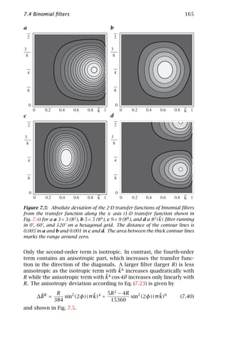
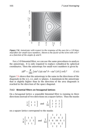
![7.5 Cascaded averaging 167
on a hexagonal lattice.
The anisotropy deviation according to Eq. (7.23) is given by
R ˜
ˆ
∆ hBR ≈ sin2 (3φ)(π k)6 (7.42)
15360
for small wave numbers. Figure 7.5d shows that the anisotropy for B2
is already about 10 times lower than for the same filter on a square
grid. The maximum anisotropy is well below 0.01 even for this small
filter.
7.4.4 Efficient computation
We close our consideration of binomial filters with some remarks on
fast algorithms. A direct computation of a BR operator with (R + 1)D
filter coefficients requires (R + 1)D multiplications and (R + 1)D − 1 addi-
tions. If we decompose the binomial mask into elementary smoothing
masks B = 1/2 [1 1] and apply this mask in all directions R times each,
we only need DR additions. All multiplications can be handled much
more efficiently as shift operations. For example, the computation of a
9 × 9 (9 × 9 × 9) binomial filter requires only 16 (24) additions and some
shift operations compared to 81 (729) multiplications and 80 (728) ad-
ditions needed for the direct approach.
7.5 Cascaded averaging
The approaches discussed so far for local averaging are no solution if
the averaging should cover large neighborhoods for the following rea-
sons: First, binomial filters are not suitable for large-scale averaging—
despite their efficient implementation by cascaded convolution with
B—because the averaging distance increases only with the square root
of the mask size (see Eq. (7.34) in Section 7.4.1). Secondly, box filters
and recursive filters are, in principle, suitable for large-scale averaging
because the number of operations does not increase with the size of the
point spread function (operation of the order O(R 0 )). However, both
types of filters have a nonideal transfer function. The transfer function
of the box filter is not monotonically decreasing with the wave number
(Section 7.3) and both filters show too large deviations from an isotropic
response. In this section, two techniques are discussed for large-scale
averaging that overcome these deficits and limitations, multistep aver-
aging (Section 7.5.1) and multigrid averaging (Section 7.5.2).
7.5.1 Multistep averaging
The problem of slow large-scale averaging originates from the small
distance between the pixels averaged by small masks. In order to over-
come this problem, we may use the same elementary averaging process](https://image.slidesharecdn.com/computervision-handbookofcomputervisionandapplicationsvolume2-signalprocessingandpatternrecognition-120205081400-phpapp02/85/Computer-vision-handbook-of-computer-vision-and-applications-volume-2-signal-processing-and-pattern-recognition-192-320.jpg)
![168 7 Local Averaging
a b
Figure 7.7: Transfer functions of the binomial filter B4 (B = 1/16[1 4 6 4 1]) and
the same filter stretched by a a factor of two, B4 (B2 = 1/16[1 0 4 0 6 0 4 0 1]),
2
and b a factor of four, B4 .
4
but with more distant pixels. As the box, binomial and recursive aver-
aging filters are separable and thus are applied as cascaded filter oper-
ations running one after the other in all coordinate directions through
a multidimensional signal, it is sufficient to discuss increasing the step
width for 1-D filter operations. A 1-D convolution with a mask that
operates only with every S-th pixel can be written as a stretched mask
hn n = Sn
(hS )n = ⇒ˆ ˜ ˆ ˜
⇐ hS (k) = h(k/S) (7.43)
0 else
Because of the reciprocity between the spatial and Fourier domains the
stretching of the filter mask by a factor S results in a corresponding
shrinking of the transfer function. This shrinking goes—because of the
periodicity of the transfer function of discrete samples—along with an
S-fold replication of the transfer function as illustrated in Fig. 7.7.
An averaging filter that is used with a larger step width is no longer
a good averaging filter for the whole wave-number range but only for
˜
wave numbers up to k = 1/S. Used individually, these filters are thus
not of much help. But we can use them in cascade in such a way that
previous smoothing has already removed all wave numbers beyond
˜
k = 1/S. This is the basic principle for the design of cascaded filters.
For practical design there are two degrees of freedom. First, we can
select the basic filter that is used repeatedly with different step widths.
Here, box, binomial and relaxation filters are investigated. Second, we
can choose the way in which the step width is increased. We will con-
sider both a linear and an exponential increase in the step width. Gen-
erally, a cascaded filter operation consists of the following chain of P
operations with the filter operation B:
Ba P . . . Ba p . . . B a 2 B a 1 (7.44)
P times](https://image.slidesharecdn.com/computervision-handbookofcomputervisionandapplicationsvolume2-signalprocessingandpatternrecognition-120205081400-phpapp02/85/Computer-vision-handbook-of-computer-vision-and-applications-volume-2-signal-processing-and-pattern-recognition-193-320.jpg)
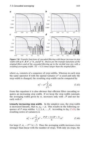
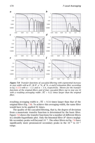
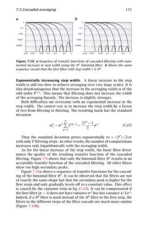
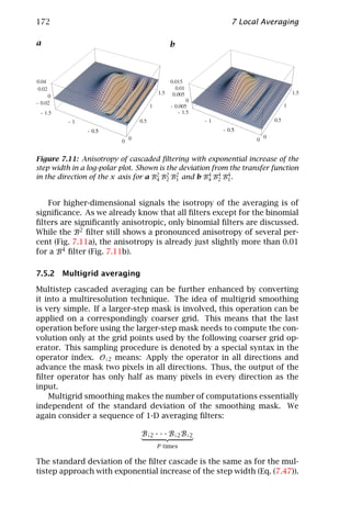
![7.6 Weighted averaging 173
ˆ ˜
Also, as long as the sampling condition is met, that is, Bp (k) = 0
˜ ≥ 1/2, the transfer functions of the filters are the same as for the
∀k
multistep filters.
If B↓2 takes q operations, the operator sequence takes
P
1 1
q = 2q 1 − P −1 < 2q (7.48)
p =1
2 p −1 2
Thus, smoothing to any degree takes no more than twice as many op-
erations as smoothing at the first step.
7.6 Weighted averaging
Image data, just like any other experimental data, may be characterized
by individual errors that have to be considered in any further process-
ing. As an introduction, we first discuss the averaging of a set of N
data gn with standard deviations σn . From elementary statistics, it is
known that appropriate averaging requires the weighting of each data
2
point gn with the inverse of the variance wn = 1/σn . Then, an estimate
of the mean value is given by
N N
2 2
g = gn /σn 1/σn (7.49)
n=1 n=1
while the standard deviation of the mean is
N
σ 2g = 1 2
1/σn (7.50)
n=1
The application of weighted averaging to image processing is known
as normalized convolution [3]. The averaging is now extended to a local
neighborhood. Each pixel enters the convolution sum with a weighting
factor associated with it. Thus, normalized convolution requires two
signals. One is the image G to be processed, the other an image W with
the weighting factors.
By analogy to Eqs. (7.49) and (7.50), normalized convolution with
the mask H is defined as
H ∗ (W · G)
G = (7.51)
H∗W
A normalized convolution with the mask H essentially transforms the
image G and the weighting image W into a new image G and a new
weighting image W = H ∗ W , which can undergo further processing.
Normalized convolution is just adequate consideration of pixels
with spatially variable statistical errors. “Standard” convolution can](https://image.slidesharecdn.com/computervision-handbookofcomputervisionandapplicationsvolume2-signalprocessingandpatternrecognition-120205081400-phpapp02/85/Computer-vision-handbook-of-computer-vision-and-applications-volume-2-signal-processing-and-pattern-recognition-198-320.jpg)
![174 7 Local Averaging
be regarded as a special case of normalized convolution. Then all pix-
els are assigned the same weighting factor and it is not required to use
a weighting image, because the factor remains a constant.
The flexibility of normalized convolution is given by the choice of
the weighting image. The weighting image is not necessarily associ-
ated with an error. It can be used to select and/or amplify pixels with
certain features. In this way, normalized convolution becomes a versa-
tile nonlinear operator. The application of normalized convolution is
discussed in a number of contributions in Volume 3 of this handbook:
Sections 30.3.4, 32.4.4, 33.4.3, and 37.4.2.
7.7 References
[1] Oppenheim, A. V. and Schafer, R. W., (1989). Discrete-time Signal Process-
ing. Prentice-Hall Signal Processing Series. Englewood Cliffs, NJ: Prentice-
Hall.
[2] Jähne, B., (1997). Handbook of Digital Image Processing for Scientific Ap-
plications. Boca Raton, FL: CRC Press.
[3] Granlund, G. H. and Knutsson, H., (1995). Signal Processing for Computer
Vision. Norwell, MA: Kluwer Academic Publishers.](https://image.slidesharecdn.com/computervision-handbookofcomputervisionandapplicationsvolume2-signalprocessingandpatternrecognition-120205081400-phpapp02/85/Computer-vision-handbook-of-computer-vision-and-applications-volume-2-signal-processing-and-pattern-recognition-199-320.jpg)
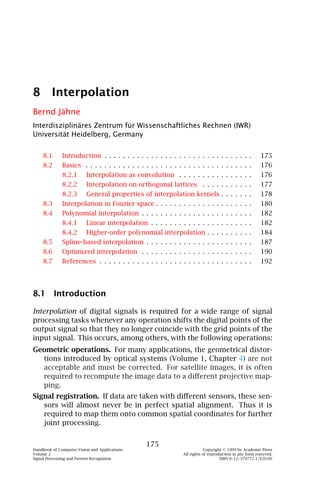
![176 8 Interpolation
Multiresolution signal processing. For multigrid data structures, such
as pyramids (Section 4.4), signals are represented at different reso-
lution levels. On such data structures it is necessary to interpolate
missing points from coarser levels to be able to process them at a
finer level.
Coarse-to-fine strategies. Coarse-to-fine strategies are an often used
concept on multigrid data structures if the processing involves im-
ages that are shifted to each other either because of a different sen-
sor (image registration), a different perspective (stereo images) or
motion of objects (Chapter 13). In all these cases it is required to
warp the images with the determined displacement vector field be-
fore processing at the next finer resolution (Chapter 14).
Test image generation. In order to evaluate algorithms, it is important
to apply them to known signals. For image sequence processing,
for example, it is useful to simulate displacement vector fields by
warping images correspondingly.
For a long time there was little effort put into interpolation algo-
rithms for computer vision. Thus most of the available procedures have
been invented for computer graphics in the framework of photorealistic
rendering. An excellent survey in this respect is provided by Wolberg
[1]. Only with increasing demand for subpixel-accurate computer vi-
sion algorithms have the researchers became aware of the importance
of accurate interpolation algorithms. The demands are quite high. As
a rule of thumb, interpolation should neither change the amplitude of
a signal by more than 1 % nor shift any signal by more than 0.01.
8.2 Basics
8.2.1 Interpolation as convolution
The basis of interpolation is the sampling theorem (Section 2.4.2). This
theorem states that the digital signal completely represents the contin-
uous signal provided the sampling conditions are met. This basic fact
suggests the following general framework for interpolation:
Reconstruction of continuous signal. From the sampled signal a con-
tinuous or a higher-resolution representation is reconstructed.
Filtering. Before a resampling can be performed, it is necessary to
check whether a prefiltering of the data is required. Whenever the
data is to be resampled with a coarser resolution, aliasing could oc-
cur because the sampling condition is no longer met (Section 2.4.3).
Resampling. This step finally forms the new digital signal.
Of course, a certain procedure for interpolation can perform two or
even all of these steps in a single operation. However, it is still helpful](https://image.slidesharecdn.com/computervision-handbookofcomputervisionandapplicationsvolume2-signalprocessingandpatternrecognition-120205081400-phpapp02/85/Computer-vision-handbook-of-computer-vision-and-applications-volume-2-signal-processing-and-pattern-recognition-201-320.jpg)
![8.2 Basics 177
for a better understanding of the procedure to separate it into these
steps.
Although these procedures sound simple and straightforward, they
are not. The problem is related to the fact that the reconstruction of the
continuous signal from the sampled signal in practice is quite involved
and can be performed only approximately. Thus, we need to balance the
computational effort with the residual error for a given interpolation
task.
Generally, a continuous multidimensional signal is interpolated from
values at all points of a lattice by (Section 2.4.4)
P
gr (x) = gs (r n + s p )h(x − (r n + s p )) (8.1)
p =1 n
In this equation r n are the translation vectors of the lattice and s p the
offsets of the P points in the primitive cell of the lattice. If a continuous
signal is required but only the value at a shifted point p (Eq. (8.1))
reduces to
P
gr (p) = gs (r n + s p )h(p − (r n + s p )) (8.2)
p =1 n
This equation reveals that interpolation is nothing else but a general-
ized convolution operation of the points on a discrete lattice with sam-
pled values from the interpolation kernel. The only difference is that
the result of the operation is not written back to the same lattice but to
a shifted lattice. Thus an interpolation operation can be described by
a transfer function. According to the discussion of the sampling theo-
rem in Sections 2.4.2 and 2.4.4, the ideal interpolation function has a
transfer function that is constantly one within the first Brillouin zone
and zero outside.
8.2.2 Interpolation on orthogonal lattices
For the rest of this chapter, we will restrict all considerations to orthog-
onal lattices because interpolation of multidimensional signals is much
easier to handle on these grids. On an orthogonal lattice with only one
point per primitive cell (P = 1), the interpolation in Eq. (8.1) reduces to
˜
gr (x) = ˜
gs (n)h(x − n) (8.3)
n
In this equation all vectors in the spatial domain are expressed in units
˜
of the lattice constants: xd = xd /∆xd . Thus, the components of the
translation vector r are integers and are replaced by n = [n1 , . . . , nD ]T ,](https://image.slidesharecdn.com/computervision-handbookofcomputervisionandapplicationsvolume2-signalprocessingandpatternrecognition-120205081400-phpapp02/85/Computer-vision-handbook-of-computer-vision-and-applications-volume-2-signal-processing-and-pattern-recognition-202-320.jpg)
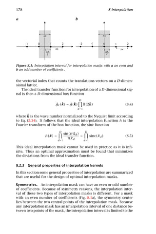
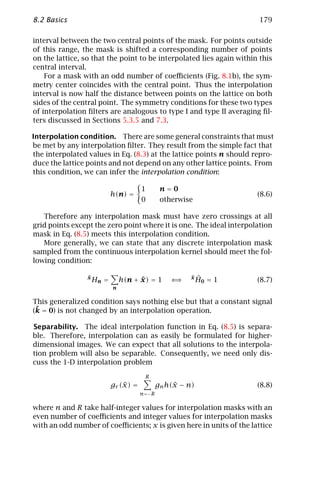

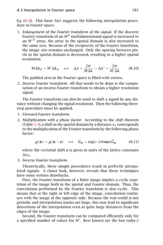
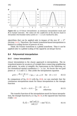
![8.4 Polynomial interpolation 183
A comparison with the ideal transfer function for interpolation Eq. (8.4),
see also Fig. 8.2b, shows that two distortions are introduced by linear
interpolation:
˜
1. While low wave numbers (and especially the mean value k = 0) are
interpolated correctly, high wave numbers are reduced in ampli-
˜
tude, resulting in some degree of smoothing. At k = 1, the transfer
ˆ 1 (1) = (2/π )2 ≈ 0.4.
function is reduced to about 40 %: h
ˆ ˜ ˜
2. As h1 (k) is not zero at wave numbers k > 1, some spurious high
wave numbers are introduced. If the continuously interpolated im-
age is resampled, this yields moderate aliasing. The first sidelobe
has an amplitude of (2/3π )2 ≈ 0.045.
˜
If we interpolate only the intermediate grid points at x = 0, the
continuous interpolation function Eq. (8.13) reduces to a discrete con-
˜
volution mask with values at x = [. . . − 3/2 − 1/2 1/2 3/2 . . . ]. As
˜
Eq. (8.13) is zero for |x | ≥ 1, we obtain the simple interpolation mask
H = 1/2[1 1] with the transfer function
ˆ ˜ ˜
H1 (k) = cos π k/2 (8.15)
The transfer function is real, so no phase shifts occur. The signifi-
cant amplitude damping at higher wave numbers, however, shows that
structures with high wave numbers are not correctly interpolated.
Phase shifts do occur at all other values except for the intermedi-
˜
ate grid points at x = 0. We investigate the phase shift and amplitude
attenuation of linear interpolation at arbitrary fractional integer shifts
∈ [−1/2, 1/2]. This results in the following mask and transfer func-
tion for linear interpolation:
[(1/2 − ) (1/2 + )] ⇐⇒ ˆ ˜ ˜ ˜
h1 ( , k) = cos π k/2 + 2i sin π k/2
(8.16)
The mask contains a symmetric part [1/2 1/2] and an antisymmetric
part [− ]. In order to estimate the error in the phase shift, it is
˜
useful to compensate for the linear phase shift ∆ϕ = π k caused by
the displacement . Then we obtain
ˆ ˜ ˜ ˜ ˜
h1 ( , k) = (cos π k/2 + 2i sin π k/2) exp(−i π k) (8.17)
˜
A Taylor expansion in k helps to reveal the amplitude response
1/2 1−4 2
ˆ ˜ ˜
h1 ( , k) = cos2 π k/2 + 4 2 ˜
sin2 π k/2 ≈1− ˜
(π k)2
8
(8.18)
and phase error ∆ϕ
(1 − 4 2)
∆ϕ ≈ ˜
(π k)3 (8.19)
12](https://image.slidesharecdn.com/computervision-handbookofcomputervisionandapplicationsvolume2-signalprocessingandpatternrecognition-120205081400-phpapp02/85/Computer-vision-handbook-of-computer-vision-and-applications-volume-2-signal-processing-and-pattern-recognition-208-320.jpg)
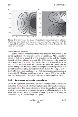
![8.4 Polynomial interpolation 185
For symmetry reasons, the lattice points are placed at the positions
˜ 2p − P
kp = (8.21)
2
For an even number of points (P is odd), the lattice points are located
at half-integer values.
˜
From the interpolation condition at the grid points gr (kp ) = gp , we
obtain a linear equation system with P +1 equations and P +1 unknowns
aP of the following form when P is odd:
g0 1 −P /2 P 2 /4 −P 3 /8 · · · a0
. . .
. . .
. . .
g 1 −1/2 1/4 −1/8 · · · (P −1)/2
a
(P −1)/2
= (8.22)
g(P +1)/2 1 1/2 1/4 1/8 · · · a(P +1)/2
. . .
.
. . .
. .
gP 1 P /2 P 2 /4 P 3 /8 · · · aP
or written as a matrix equation:
p
2q − P
g = Ma with Mpq = , p, q ∈ [0, P ] (8.23)
2
For a cubic polynomial (P = 3), the solution of the equations system
is
a0 −3 27 27 −3 g0
a1 −2 g1
= 1 2 −54 54 (8.24)
a2 48 12 −12 −12 12 g2
a3 −8 24 −24 8 g3
Using Eqs. (8.20) and (8.24) we can express the interpolated values
for the position in the interval [−1/2, 1/2] as
9−4 2 1−4 2
g( ) = (g1 + g2 ) − (g0 + g3 )
16 16
(8.25)
(9 − 4 2) (1 − 4 2)
+ (g2 − g1 ) − (g3 − g0 )
8 24
Thus the interpolation mask is
−α α 8+α (8 + α) 8+α (8 + α) −α α
+ , + , − , − (8.26)
16 24 16 8 16 8 16 24
with α = 1 − 4 2. For = 0 (α = 1), the mask reduces to
1
[−1 9 9 − 1] (8.27)
16](https://image.slidesharecdn.com/computervision-handbookofcomputervisionandapplicationsvolume2-signalprocessingandpatternrecognition-120205081400-phpapp02/85/Computer-vision-handbook-of-computer-vision-and-applications-volume-2-signal-processing-and-pattern-recognition-210-320.jpg)
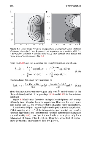
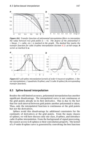
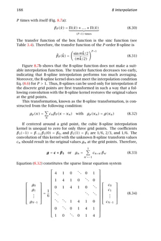
![8.5 Spline-based interpolation 189
using cyclic boundary conditions. The determination of the B-spline
transformation thus requires the solution of a linear equation system
with N unknowns. The special form of the equation system as a con-
volution operation, however, allows for a more efficient solution. In
Fourier space, Eq. (8.33) reduces to
ˆ ˆc
g = β3 ˆ (8.35)
ˆ ˜ ˜
The transfer function of β3 is β3 (k) = 2/3 + 1/3 cos(π k). As this func-
tion has no zeroes, we can compute c by inverse filtering, that is, con-
voluting g with a mask that has the transfer function
ˆ− ˜ ˆ ˜ 1
β3 1 (k) = βT (k) = (8.36)
˜
2/3 + 1/3 cos(π k)
This is the transfer function of a recursive relaxation filter (Section 5.4.6)
that is applied first in the forward and then in the backward direction
with the following recursion [2]:
√
gn = gn − (2 − 3)(gn−1 − gn )
√ (8.37)
cn = gn − (2 − 3)(cn+1 − gn )
The entire operation takes only two multiplications and four additions.
The B-spline interpolation is applied after the B-spline transforma-
tion. In the continuous cubic case this yields the effective transfer func-
tion using Eqs. (8.31) and (8.36),
˜ ˜
sin4 (π k/2)/(π k/2)4
ˆ ˜
βI (k) = (8.38)
˜
(2/3 + 1/3 cos(π k))
Essentially, the B-spline transformation performs an amplification
˜
of high wave numbers (at k = 1 by a factor 3), which compensates the
smoothing of the B-spline interpolation to a large extent.
We investigate this compensation at both the grid points and the
intermediate points. From the equation of the cubic B-spline interpo-
lating kernel (Eq. (8.30); see also Fig. 8.7a) the interpolation coefficients
for the grid points and intermediate grid points are
1/6 [1 4 1] and 1/48 [1 23 23 1] (8.39)
respectively. Therefore, the transfer functions are
˜
2/3 + 1/3 cos(π k) ˜ ˜
and 23/24 cos(π k/2) + 1/24 cos(3π k/2) (8.40)
respectively. At the grid points, the transfer functions compensate
exactly—as expected—the application of the B-spline transformation
Eq. (8.36). Thus, the interpolation curve goes through the values at the](https://image.slidesharecdn.com/computervision-handbookofcomputervisionandapplicationsvolume2-signalprocessingandpatternrecognition-120205081400-phpapp02/85/Computer-vision-handbook-of-computer-vision-and-applications-volume-2-signal-processing-and-pattern-recognition-214-320.jpg)
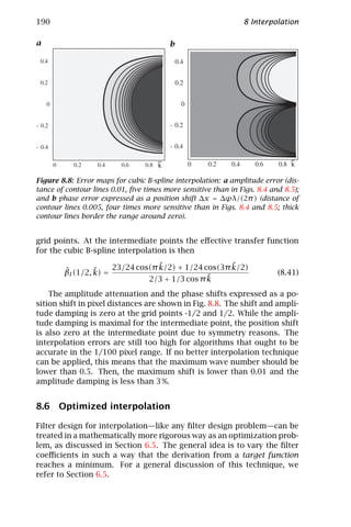
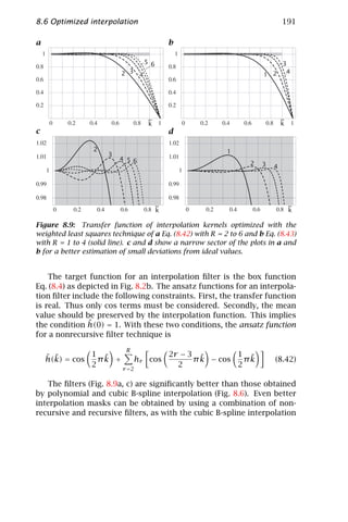
![192 8 Interpolation
(compare also Example 6.2 in Section 6.5.1):
R
˜
cos 1/2 π k + ˜ ˜
hr cos (2r − 3)/2 π k − cos 1/2 π k
ˆ ˜ r =2
h(k) =
˜
1 − α + α cos π k
(8.43)
Figure 8.9b, d shows the transfer functions for R = 1 to 4. A more
detailed discussion of interpolation filters including tables with opti-
mized filters can be found in Jähne [3].
8.7 References
[1] Wolberg, G., (1990). Digital Image Warping. Los Alamitos, CA: IEEE Com-
puter Society Press.
[2] Unser, M., Aldroubi, A., and Eden, M., (1991). Fast B-spline transforms for
continuous image representation and interpolation. IEEE Trans. PAMI, 13:
277–285.
[3] Jähne, B., (1997). Handbook of Digital Image Processing for Scientific Ap-
plications. Boca Raton, FL: CRC Press.](https://image.slidesharecdn.com/computervision-handbookofcomputervisionandapplicationsvolume2-signalprocessingandpatternrecognition-120205081400-phpapp02/85/Computer-vision-handbook-of-computer-vision-and-applications-volume-2-signal-processing-and-pattern-recognition-217-320.jpg)
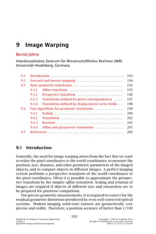
![194 9 Image Warping
a b
input image output image input image output image
Figure 9.1: Illustration of: a forward mapping; and b inverse mapping for spa-
tial transformation of images. With forward mapping, the value at an output
pixel must be accumulated from all input pixels that overlap it. With inverse
mapping, the value of the output pixel must be interpolated from a neighbor-
hood in the input image.
pixel distance is feasible. To maintain this accuracy, all geometric trans-
formations applied to digital images must preserve this high position
accuracy. This demand goes far beyond the fact that no distortions
are visible in the transformed images as it is required for computer
graphics applications.
Image warping is a widely neglected subject in computer vision.
Thus it is not surprising that many of the available techniques have
been developed within the frame of computer graphics applications,
especially for the mapping of textures onto objects. Image warping
is treated in detail in a monograph by Wolberg [1] and also studied in
Gomes and Velho [2]. This chapter covers the basics of geometric trans-
forms (Section 9.3) and discusses fast algorithms for scaling, rotation
and affine transforms of images (Section 9.4). All of these algorithms
can be used with various techniques of subpixel accurate interpolation.
This subject is treated in Chapter 8.
9.2 Forward and inverse mapping
A geometric transform defines the relationship between the points in
two images. This relation can be expressed in two ways. Either the
coordinates of the output image x can be specified as a function of
the coordinates of the input image x or vice versa:
x = M(x) forward mapping
−1
(9.1)
x = M (x ), inverse mapping
where M specifies the mapping function and M −1 its inverse. The two
expressions in Eq. (9.1) give rise to two principal ways of spatial trans-
formations: forward mapping and inverse mapping.](https://image.slidesharecdn.com/computervision-handbookofcomputervisionandapplicationsvolume2-signalprocessingandpatternrecognition-120205081400-phpapp02/85/Computer-vision-handbook-of-computer-vision-and-applications-volume-2-signal-processing-and-pattern-recognition-219-320.jpg)
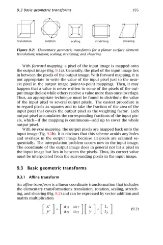
![196 9 Image Warping
With homogeneous coordinates [3, 4], the affine transform is written
with a single matrix multiplication as
x a11 a12 tx x
y = a21 a22 ty y (9.3)
1 0 0 1 1
An affine transform has six degrees of freedom: two for translation
(tx , ty ) and one each for rotation, scaling, stretching, and shearing (a11 ,
a12 , a21 , and a22 ). The affine transform maps a triangle into a triangle
and a rectangle into a parallelogram. Therefore, it is also referred to
as three-point mapping. Thus, it is obvious that the use of the affine
transform is restricted. More general distortions such as the mapping
of a rectangle into an arbitrary quadrilateral are not affine transforms.
9.3.2 Perspective transform
Perspective projection is the basis of geometric optical imaging as dis-
cussed in Volume 1, Chapter 4. The affine transform corresponds to
parallel projection and can only be used as a model for optical imaging
in the limit of a small field of view. The general perspective transform
is most conveniently written with homogeneous coordinates as
w x a11 a12 a13 wx
w y = a21 a22 a23 wy or X = P X (9.4)
w a31 a32 1 w
The two additional coefficients a31 and a32 in comparison to the
affine transform Eq. (9.3) describe the perspective projection.
Written in standard coordinates, the perspective transform accord-
ing to Eq. (9.4) reads as
a11 x + a12 y + a13
x =
a31 x + a32 y + 1
(9.5)
a21 x + a22 y + a23
y =
a31 x + a32 y + 1
In contrast to the affine transform, the perspective transform is non-
linear. However, it is reduced to a linear transform by using homoge-
neous coordinates. A perspective transform maps lines into lines but
only lines parallel to the projection plane remain parallel. A rectangle
is mapped into an arbitrary quadrilateral. Therefore, the perspective
transform is also referred to as four-point mapping.](https://image.slidesharecdn.com/computervision-handbookofcomputervisionandapplicationsvolume2-signalprocessingandpatternrecognition-120205081400-phpapp02/85/Computer-vision-handbook-of-computer-vision-and-applications-volume-2-signal-processing-and-pattern-recognition-221-320.jpg)
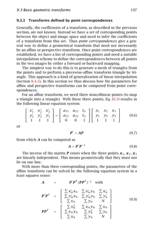
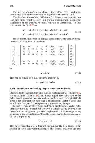
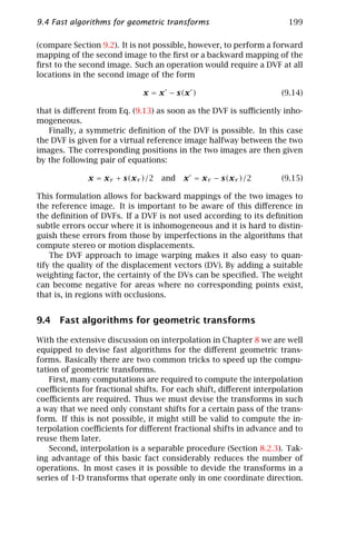
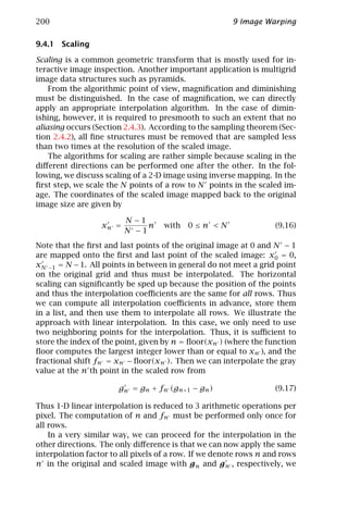
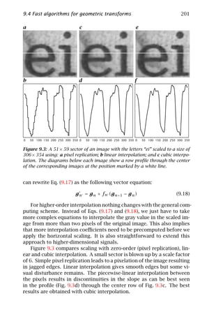
![202 9 Image Warping
9.4.2 Translation
Translation is the simplest of all geometric transformations and does
not require much consideration. The shift is the same for all pixels.
Thus, we need only one set of interpolation coefficients that is applied
to each pixel. As for scaling, we perform first the horizontal shift and
then the vertical shift. Note that interpolation algorithms applied in
this way have the same computational structure as a convolution oper-
ator. Therefore, we can use the same efficient storage scheme for the
horizontally shifted or scaled rows as in Section 5.6 for neighborhood
operators.
9.4.3 Rotation
With rotation it is less obvious how it can be decomposed into a se-
quence of one-dimensional geometrical transforms. Indeed, there are
several possibilities. Interestingly, these algorithms have not been in-
vented in the context of image processing but for computer graphics.
Catmull and Smith [5] suggested the following 2-pass shear-scale
transform:
cos θ sin θ 1 0 cos θ sin θ
R= = (9.19)
− sin θ cos θ − tan θ 1/ cos θ 0 1
The first matrix performs a horizontal shear/scale operation, and the
second, a vertical shear/scale operation. Written in components, the
first transform is
x = x cos θ + y sin θ
(9.20)
y = y
The image is shifted horizontally by the offset y sin θ and is diminished
by the factor of x cos θ. Thus Eq. (9.20) constitutes a combined shear-
scale transform in horizontal direction only (Fig. 9.4).
Likewise, the second transform
x = x
(9.21)
y = y / cos θ − x tan θ
performs a combined shear-scale transform in vertical direction only.
This time, the image is enlarged in vertical direction by the factor of
1/ cos θ.
This usage of scaling operations for image rotation has two disad-
vantages. First, the scale operations require extra computations since
the image need not only be shifted but also scaled. Second, although
the size of an image does not change during a rotation, the first scaling
reduces the size of the image in horizontal direction and thus could](https://image.slidesharecdn.com/computervision-handbookofcomputervisionandapplicationsvolume2-signalprocessingandpatternrecognition-120205081400-phpapp02/85/Computer-vision-handbook-of-computer-vision-and-applications-volume-2-signal-processing-and-pattern-recognition-227-320.jpg)
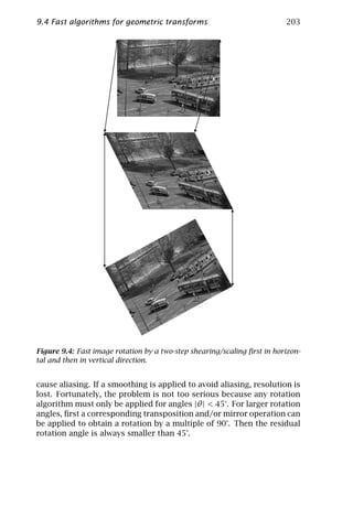
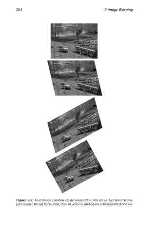
![9.4 Fast algorithms for geometric transforms 205
With a 3-pass transform [6, 7], rotation can be decomposed into
three 1-D shear transforms avoiding scaling (Fig. 9.5):
cos θ sin θ
R =
− sin θ cos θ
(9.22)
1 tan(θ/2) 1 0 1 tan(θ/2)
=
0 1 − sin θ 1 0 1
9.4.4 Affine and perspective transforms
A 2-D affine transform adds three more degrees of freedom to a simple
transform that includes only rotation and translation. These are two
degrees of freedom for scaling in x and y direction, and one degree of
freedom for shearing. Together with the degree of freedom for rota-
tion, we have (without the translation) four degrees of freedom that can
generally be described by a 2 × 2 matrix as discussed in Section 9.3.1:
a11 a12
A= (9.23)
a21 a22
One way to perform an affine transform efficiently is to decompose it
into a rotation, shear, and scaling transform:
a11 a12 sx 0 1 s cos θ sin θ
A= = (9.24)
a21 a22 0 sy 0 1 − sin θ cos θ
The parameters sx , sy , s, and θ can be computed from the matrix co-
efficients by
det(A)
sx = a2 + a2
11 21 sy =
sx
(9.25)
a11 a12 + a21 a22 a21
s = tan θ = −
det(A) a11
where det(A) is the determinant of the matrix A. The shear transform
and the rotation can be computed simultaneously by the 3-pass shear
transform discussed in Section 9.4.3 with the following modification to
Eq. (9.22):
1 s cos θ sin θ
R =
0 1 − sin θ cos θ
1 s + tan(θ/2) 1 0 1 tan(θ/2)
=
0 1 − sin θ 1 0 1
(9.26)](https://image.slidesharecdn.com/computervision-handbookofcomputervisionandapplicationsvolume2-signalprocessingandpatternrecognition-120205081400-phpapp02/85/Computer-vision-handbook-of-computer-vision-and-applications-volume-2-signal-processing-and-pattern-recognition-230-320.jpg)
![206 9 Image Warping
Thus the affine transform can be computed with a 3-pass shear trans-
form Eq. (9.26) followed by a scaling transform as discussed in Sec-
tion 9.4.1. Fast algorithms for perspective and more general transforms
are treated in detail in Wolberg [1].
9.5 References
[1] Wolberg, G., (1990). Digital image warping. Los Alamitos, CA: IEEE Com-
puter Society Press.
[2] Gomes, J. and Velho, L., (1997). Image Processing for Computer Graphics.
New York: Springer.
[3] Foley, J. D., van Dam, A., Feiner, S. K., and Hughes, J. F., (1990). Computer
Graphics, Principles and Practice. Reading, MA: Addison Wesley.
[4] Watt, A., (1990). Fundamentals of three-dimensional computer graphics.
Workingham, England: Addison-Wesley.
[5] Catmull, E. and Smith, A. R., (1980). 3-D transformations of images in
scanline order. Computer Graphics (SIGGRAPH ’80 Proceedings), 14:279–
285.
[6] Paeth, A. W., (1986). A fast algorithm for general raster rotation. In Graph-
ics Interface ’86, pp. 77–81.
[7] Tanaka, A., Kameyama, M., Kazama, S., and Watanabe, O., (1986). A rotation
method for raster image using skew transformation. In Proc. IEEE Conf.
Computer Vision and Pattern Recognition (CVPR’86), pp. 272–277. IEE, IEEE
Computer Society Press.](https://image.slidesharecdn.com/computervision-handbookofcomputervisionandapplicationsvolume2-signalprocessingandpatternrecognition-120205081400-phpapp02/85/Computer-vision-handbook-of-computer-vision-and-applications-volume-2-signal-processing-and-pattern-recognition-231-320.jpg)


![210 10 Local Structure
ko xC
xB
xA
Figure 10.1: Illustration of a linear symmetric or simple neighborhood. The
¯
gray values depend only on a coordinate given by a unit vector r .
10.1 Introduction
The analysis of the structure in small neighborhoods is a key element
in higher-dimensional signal processing. Changes in the gray values
reveal either the edge of an object or the type of texture.
10.2 Properties of simple neighborhoods
10.2.1 Representation in the spatial domain
The mathematical description of a local neighborhood by continuous
functions has two significant advantages. First, it is much easier to for-
mulate the concepts and to study their properties analytically. As long
as the corresponding discrete image satisfies the sampling theorem, all
the results derived from continuous functions remain valid because the
sampled image is an exact representation of the continuous gray-value
function. Second, we can now distinguish between errors inherent to
the chosen approach and those that are only introduced by the dis-
cretization.
A simple local neighborhood is characterized by the fact that the
gray value only changes in one direction. In all other directions it is
constant. Because the gray values are constant along lines and form
oriented structures this property of a neighborhood is denoted as local
orientation [1] or linear symmetry [2]. Only more recently, the term
simple neighborhood has been coined by Granlund and Knutsson [3].
If we orient the coordinate system along the principal directions,
the gray values become a 1-D function of only one coordinate. Gener-
ally, we will denote the direction of local orientation with a unit vector](https://image.slidesharecdn.com/computervision-handbookofcomputervisionandapplicationsvolume2-signalprocessingandpatternrecognition-120205081400-phpapp02/85/Computer-vision-handbook-of-computer-vision-and-applications-volume-2-signal-processing-and-pattern-recognition-235-320.jpg)
![212 10 Local Structure
between the two domains, its thickness is inversely proportional to
the size of the window. From this elementary relation, we can already
conclude qualitatively that the accuracy of the orientation estimate is
directly related to the ratio of the window size to the wavelength of the
smallest structures in the window.
10.2.3 Direction versus orientation
For an appropriate representation of simple neighborhoods, it is first
important to distinguish orientation from direction. The direction is
defined over the full angle range of 2π (360°). Two vectors that point
in opposite directions, that is, differ by 180°, are different. The gradient
vector, for example, always points into the direction into which the gray
values are increasing. With respect to a bright object on a dark back-
ground, this means that the gradient at the edge is pointing towards the
object. In contrast, to describe the direction of a local neighborhood,
an angle range of 360° makes no sense. We cannot distinguish between
patterns that are rotated by 180°. If a pattern is rotated by 180°, it still
has the same direction. Thus, the direction of a simple neighborhood
is different from the direction of a gradient. While for the edge of an
object gradients pointing in opposite directions are conflicting and in-
consistent, for the direction of a simple neighborhood this is consistent
information.
In order to distinguish the two types of “directions,” we will speak
of orientation in all cases where an angle range of only 180° is required.
Orientation is still, of course, a cyclic quantity. Increasing the orienta-
tion beyond 180° flips it back to 0°. Therefore, an appropriate repre-
sentation of orientation requires an angle doubling.
In his pioneering paper on a general picture processing operator
Granlund [1] introduced a vectorial representation of the local orien-
tation. The magnitude of the orientation vector is set to the certainty
with which the orientation could be determined and its direction to the
doubled orientation angle. This vector representation of orientation
has two significant advantages.
First, it is more suitable for further processing than a separate rep-
resentation of the orientation by two scalar quantities. Take, for ex-
ample, averaging. Vectors are summed up by chaining them together,
and the resulting sum vector is the vector from the starting point of
the first vector to the end point of the last vector. The weight of an
individual vector in the vector sum is given by its length. In this way,
the certainty of the orientation measurement is adequately taken into
account. In a region with homogeneous orientation the vectors line up
to a large vector, that is, give a certain orientation estimate. However,
in a region with randomly distributed orientation the resulting vector
remains small, indicating that no significant local orientation is present.](https://image.slidesharecdn.com/computervision-handbookofcomputervisionandapplicationsvolume2-signalprocessingandpatternrecognition-120205081400-phpapp02/85/Computer-vision-handbook-of-computer-vision-and-applications-volume-2-signal-processing-and-pattern-recognition-237-320.jpg)
![10.3 Edge detection by first-order derivatives 215
Nonselective derivation. Intuitively, we expect that any derivative
operator amplifies smaller scales more strongly than coarser scales, as
the transfer function of a first-order derivative operator goes with k.
However, this condition is a too restrictive. Imagine that we first apply
a smoothing operator to an image before we apply a derivative oper-
ator. Then the resulting transfer function would not increase mono-
tonically with the wave number but decrease for higher wave numbers.
We would, however, still recognize the joint operation as a derivation
because the mean gray value is suppressed and the operator is only
sensitive to spatial gray-value changes.
Thus a more general condition is required. Here we suggest
ˆ ˜ ˜ ˆ ˜
H(k) = iπ kd B(|k|) with ˆ
B(0) = 1 and ˆ
B=0 (10.11)
This condition ensures that the transfer function is still zero for the
˜
wave number zero and increases in proportion to kd for small wave
numbers. One can regard Eq. (10.11) as a first-order derivative filter
regularized by an isotropic smoothing filter.
Isotropy. For good edge detection, it is important that the response of
the operator does not depend on the direction of the edge. If this is the
case, we speak of an isotropic edge detector. The isotropy of an edge
detector can best be analyzed by its transfer function. Equation (10.11),
which we derived from the condition of nonselective derivation, gives
a general form for an isotropic first-order derivative operator.
10.3.2 First-order difference operators
This is the simplest of all approaches to compute a gradient vector.
For the first partial derivative in the x direction, one of the following
approximations may be used:
∂g(x) ¯
g(x) − g(x − ∆xd e d )
≈ backward
∂xd ∆xd
¯
g(x + ∆xd e d ) − g(x)
≈ forward (10.12)
∆xd
¯ ¯
g(x + ∆xd e d ) − g(x − ∆xd e d )
≈ symmetric
2∆xd
¯
where e d is a unit vector in the direction d. These approximations
correspond to the filter masks
−
Dd = [1• − 1] , + Dd = [1 − 1• ] , D2d = 1/2 [1 0 − 1] (10.13)](https://image.slidesharecdn.com/computervision-handbookofcomputervisionandapplicationsvolume2-signalprocessingandpatternrecognition-120205081400-phpapp02/85/Computer-vision-handbook-of-computer-vision-and-applications-volume-2-signal-processing-and-pattern-recognition-240-320.jpg)
![216 10 Local Structure
The subscript • denotes the pixel of the asymmetric masks to which the
result is written. The symmetric difference operator results in a type III
operator (odd number of coefficients, odd symmetry, see Section 5.3.5).
The forward and backward difference operators are asymmetric and
thus not of much use in signal processing. They can be transformed in
a type IV LSI operator if the result is not stored at the position of the
right or left pixel but at a position halfway between the two pixels. This
corresponds to a shift of the grid by half a pixel distance. The transfer
function for the backward difference is then
− ˆ ˜ ˜ ˜
Dd = exp(iπ kd /2) 1 − exp(−iπ kd ) = i sin(π kd /2) (10.14)
where the first term results from the shift by half a lattice point.
According to Eq. (5.25), the transfer function of the symmetric dif-
ference operator is given by
ˆ ˜
D2d = i sin(π kd ) (10.15)
This operator can also be computed from
D2d = − Dd Bd = [1• − 1] ∗ 1/2 [1 1• ] = 1/2 [1 0 − 1]
Unfortunately, these simple difference filters are only poor approx-
imations for an edge detector. From Eq. (10.15), we infer that the mag-
nitude and direction of the gradient φ are given by
1/2
˜ ˜
| g | = sin2 (π k cos φ) + sin2 (π k sin φ) (10.16)
and
˜
sin(π k sin φ)
φ = arctan (10.17)
˜
sin(π k cos φ)
when the wave number is written in polar coordinates (k, φ). The mag-
nitude of the gradient decreases quickly from the correct value. A
˜
Taylor expansion of Eq. (10.16) in k yields for the anisotropy in the
magnitude
˜
(π k)3
∆| g | = | g(φ)| − | g(0)| ≈ sin2 (2φ) (10.18)
12
The resulting errors are shown in Fig. 10.2 as a function of the mag-
nitude of the wave number and the angle to the x axis. The decrease
is also anisotropic; it is slower in the diagonal direction. The errors
in the direction of the gradient are also large (Fig. 10.2b). While in the
direction of the axes and diagonals the error is zero, in the directions](https://image.slidesharecdn.com/computervision-handbookofcomputervisionandapplicationsvolume2-signalprocessingandpatternrecognition-120205081400-phpapp02/85/Computer-vision-handbook-of-computer-vision-and-applications-volume-2-signal-processing-and-pattern-recognition-241-320.jpg)
![10.3 Edge detection by first-order derivatives 217
a b
Figure 10.2: Anisotropy of the a magnitude and b error in the direction of
T
the gradient based on the symmetrical gradient operator D2x , D2y . The
parameters are the magnitude of the wave number (0 to 0.9) and the angle to
the x axis (0 to π /2). Distance of contour lines: a 0.02 (thick lines 0.1); b 2°.
˜
in-between it reaches values of about ± 10° already at k = 0.5. A Taylor
˜ gives in the approximation of small k the
expansion of Eq. (10.17) in k ˜
angle error
˜
(π k)2
∆φ ≈ sin 4φ (10.19)
24
From this equation, we see that the angle error is zero for φ = nπ /4
with n ∈ Z, that is, for φ = 0°, 45° 90°, . . . .
10.3.3 Roberts operator
The Roberts operator uses the smallest possible difference filters to
compute the gradients that have a common center point
1 0 0 1
Dx −y = and Dx +y = (10.20)
0 –1 –1 0
The filters Dx = [1 − 1] and Dy = [1 − 1]T are not suitable to form
a gradient operator because Dx and Dy shift the convolution result
by half a grid constant in the x and y directions, respectively. The
difference filters in diagonal direction result in a gradient vector that
is rotated by 45°. The errors in the magnitude and direction obtained
with the Roberts operator are shown in Fig. 10.3. The improvement is
only marginal as compared to the gradient computation based on the
simple difference operator D2 = 1/2 [1 0 − 1] (Fig. 10.2).](https://image.slidesharecdn.com/computervision-handbookofcomputervisionandapplicationsvolume2-signalprocessingandpatternrecognition-120205081400-phpapp02/85/Computer-vision-handbook-of-computer-vision-and-applications-volume-2-signal-processing-and-pattern-recognition-242-320.jpg)
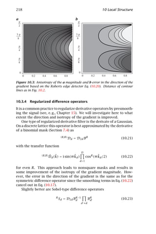
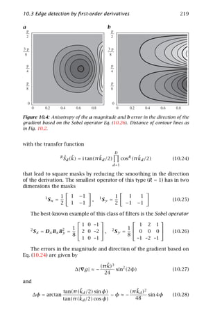
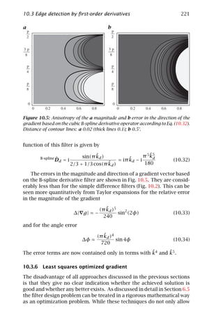
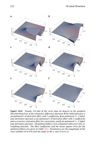
![10.4 Edge detection by zero crossings 223
Table 10.1: Gradient operators optimized for minimum error in the direction
of the gradient. The mean square error is given in units of 10−4 rad. The
lst column gives the number of operations per pixel (M = multiplication, A =
addition/subtraction). For details see Chapter 6
Name Filter coefficients Error No. Ops.
D1 [1 0 –1]/2 400 1M, 1A
Sobel [1 0 –1] ∗ [1 2 1]T /8 190 2M, 3A
opt. 7-tap [6 –31 108 0 –108 31 –6]/128 160? 3M, 3A
opt. 5-tap
[7 114 0 –114 –7]/256, α = −15/32 23 4M, 6A
+ relax
opt. Sobel [1 0 –1] ∗ [3 10 3]T /32 26 2M, 3A
opt. 5 × 5 [3 10 0 –10 –3]/32 ∗ [7 63 116 63 7]T /256 1.9 4M, 5A
the design of optimal filters, it can also be decided precisely in respect
to which criterion the solution is optimal.
Here, we will review some of the results obtained in Section 6.5 for
gradient operators that have been optimized for a minimum error in
the direction of the gradient. Figure 10.6 shows error maps of the gra-
dients angle error as a function of the wave number and direction for
six filters. Two of them, the difference operator and the Sobel operator ,
are standard solutions taken for comparison. The four other filters in-
clude two 1-D derivative operators and two Sobel-type filters with cross
smoothing. The coefficients of the filters are summarized in Table 10.1.
All optimized filters are by far superior to the standard approaches.
The mean square error in the direction of the gradient is at least one
order of magnitude lower. The clear winner for a combination of ac-
curacy and computational efficiency is the optimized 3 × 3 Sobel-type
operator that requires per filter 2 multiplications and 3 additions only.
For ultimate accuracy, the 5 × 5 Sobel-type operator is the best choice.
This filter requires about two times more operations: 4 multiplications
and 5 additions.
10.4 Edge detection by zero crossings
10.4.1 General properties
First-order derivative operators detect edges by maxima in the magni-
tude of the gradient. Alternatively, edges can be detected as zero cross-
ings of second-order derivative operators. This technique is attractive
since only linear operators are required to perform an isotropic de-
tection of edges by zero crossings. In contrast, the magnitude of the](https://image.slidesharecdn.com/computervision-handbookofcomputervisionandapplicationsvolume2-signalprocessingandpatternrecognition-120205081400-phpapp02/85/Computer-vision-handbook-of-computer-vision-and-applications-volume-2-signal-processing-and-pattern-recognition-248-320.jpg)
![224 10 Local Structure
gradient is only obtained after squaring and adding first-order deriva-
tive operators in all directions.
For an isotropic zero-crossing detector, only all second-order par-
tial derivatives must be added up. The resulting operator is called the
Laplace operator and denoted by ∆
D D
∂2 2
∆= 2
⇐⇒ − 4π 2 k2 = −4π 2 |k|
d (10.35)
d =1
∂xw d =1
From this equation it is immediately evident that the Laplace operator
is an isotropic operator.
A second-order derivative filter detects curvature. Extremes in func-
tion values should thus coincide with extremes in curvature. Conse-
quently, a second-order derivative filter should be of even symmetry
similar to a smoothing filter and all the properties for filters of even
symmetry discussed in Sections 5.3.5 and 7.2 should also apply to
second-order derivative filters. In addition, the sum of the coefficients
must be zero as for first-order derivative filters:
Hn = 0 ⇐⇒ ˆ
H(0) = 0 (10.36)
n
Also, a second-order derivative filter should not respond to a con-
stant slope. This condition implies no further constraints as it is equiv-
alent to the conditions that the sum of the coefficients is zero and that
the filter is of even symmetry.
10.4.2 Laplace of Gaussian and difference of Gaussian filters
The standard implementations for the Laplace operator are well known
and described in many textbooks (see, e. g., [4]). Thus, we will discuss
here only the question of an optimal implementation of the Laplacian
˜
operator. Because of a transfer function proportional to k2 (Eq. (10.35)),
Laplace filters tend to enhance the noise level in images considerably.
Thus, a better edge detector may be found by first smoothing the image
and then applying the Laplacian filter. This leads to a kind of regular-
ized edge detection and to two classes of filters known as Laplace of
Gaussian or LoG filters and difference of Gaussian or DoG filters. While
these filters reduce the noise level it is not clear to which extent they
improve or even optimize the isotropy of the Laplace operator.
In the discrete case, a LoG filter is approximated by first smoothing
the image with a binomial mask and then applying the discrete Laplace
filter. Thus we have the operator combination LBR with the transfer
function
D D
ˆ ˆˆ
LoG = LB R = −4 ˜
sin2 (π kd /2) ˜
cosR (π kd /2) (10.37)
d =1 d =1](https://image.slidesharecdn.com/computervision-handbookofcomputervisionandapplicationsvolume2-signalprocessingandpatternrecognition-120205081400-phpapp02/85/Computer-vision-handbook-of-computer-vision-and-applications-volume-2-signal-processing-and-pattern-recognition-249-320.jpg)
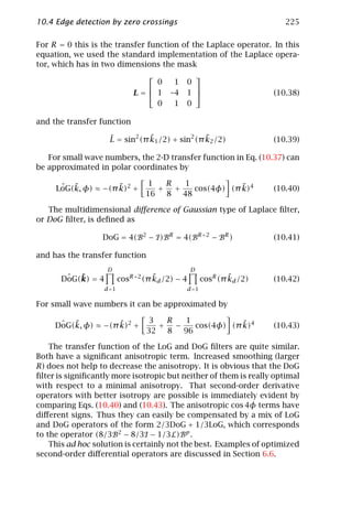
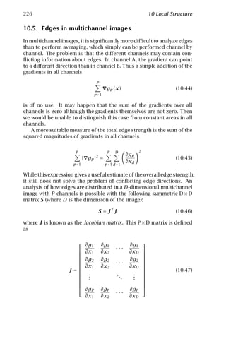
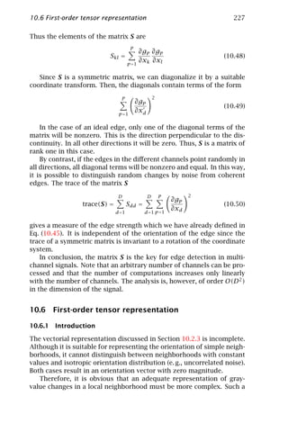
![228 10 Local Structure
representation should be able to determine a unique orientation and to
distinguish constant neighborhoods from neighborhoods without local
orientation.
In their paper on analyzing oriented patterns, Kass and Witkin [5]
started with the idea of using directional derivative filters by differen-
tiating a difference of Gaussian (DoG, Section 10.4.2) filter (written in
operator notation)
D x ( B1 − B 2 ) Rx
R(Θ) = [cos Θ sin Θ] = [cos Θ sin Θ]
D y ( B1 − B 2 ) Ry
where B1 and B2 denote two Gaussian smoothing masks with different
variances. The direction in which this directional derivative is maximal
in a mean square sense gives the orientation normal to lines of constant
gray values. This approach results in the following expression for the
variance of the directional derivative:
V (Θ) = B(R(Θ) · R(Θ)) (10.51)
The directional derivative is squared and then smoothed by a binomial
filter. This equation can also be interpreted as the inertia of an object
as a function of the angle. The corresponding inertia tensor has the
form
B(Ry · Ry ) −B(Rx · Ry )
(10.52)
−B(Rx · Ry ) B( R x · R x )
Tensorial descriptions of local structure in images were also discussed
by Bigün and Granlund [2] and Knutsson [6]. Without being aware of
the work of these authors, Rao and Schunck [7] and Rao [8] proposed
a moment tensor for the description and classification of oriented tex-
tures.
In the reminder of this chapter, several variants of tensorial descrip-
tion of local structure in multidimensional signals are discussed. The
treatment here is more general in the sense that it is not restricted to 2-
D single-channel images but that higher-dimensional and multichannel
signals are considered as well.
10.6.2 The structure tensor
A suitable representation can be introduced by a optimization strat-
egy to determine the orientation of a simple neighborhood in a slightly
more general way as performed by Kass and Witkin [5] (Section 10.6.1).
The optimum orientation is defined as the orientation that shows the
least deviations from the directions of the gradient. A suitable measure
for the deviation must treat gradients pointing in opposite directions](https://image.slidesharecdn.com/computervision-handbookofcomputervisionandapplicationsvolume2-signalprocessingandpatternrecognition-120205081400-phpapp02/85/Computer-vision-handbook-of-computer-vision-and-applications-volume-2-signal-processing-and-pattern-recognition-253-320.jpg)
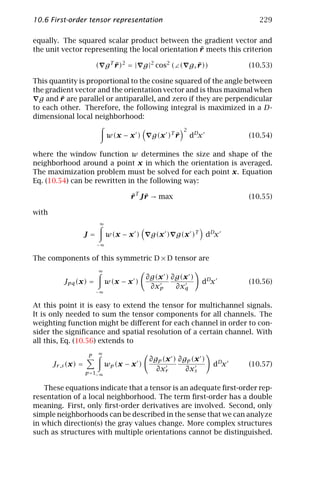
![230 10 Local Structure
The complexity of Eqs. (10.55) and (10.56) somewhat obscures their
simple meaning. The tensor is symmetric. By a rotation of the coordi-
nate system, it can be brought into a diagonal form. Then, Eq. (10.55)
reduces to
J1 1 0 ... 0 ¯
r1
0 J2 2 . . . 0 r
¯2
¯ ¯ ¯
J = r1 , r2 , . . . , rD . . .. . → max
. . . . ...
. . .
0 . . . . . . JD D ¯
rD
or
D
J= Jd d (¯d )2
r
d =1
Without loss of generality, we assume that J1 1 ≥ Jd d ∀d ≠ 1.
Then, it is obvious that the unit vector r = [1 0 . . . 0]T maximizes the
¯
foregoing expression. The maximum value is J1 1 . In conclusion, this
approach not only yields a tensor representation for the local neighbor-
hood but also shows the way to determine the orientation. Essentially,
we have to solve an eigenvalue problem. The eigenvalues λd and eigen-
vectors kd of a D × D matrix are defined by
Jkd = λd kd (10.58)
An eigenvector kd of J is thus a vector that is not turned in direc-
tion by multiplication with the matrix J, but is only multiplied by a
scalar factor, the eigenvalue λw . This implies that the structure tensor
becomes diagonal in a coordinate system that is spanned by the eigen-
vectors. For our further discussion it is important to keep in mind that
the eigenvalues are all real and nonnegative and form an orthogonal
basis [9, 10, 11].
10.6.3 Classification of local neighborhoods
The power of the tensor representation becomes apparent if we clas-
sify the eigenvalues of the structure tensor. The classifying criterion is
the number of eigenvalues that are zero. If an eigenvalue is zero, this
means that the gray values in the direction of the corresponding eigen-
vector do not change. The number of zero eigenvalues is also closely
related to the rank of a matrix. The rank of a matrix is defined as
the dimension of the subspace for which Jk ≠ 0. The space for which
Jk = 0 is denoted as the null space. The dimension of the null space
is the dimension of the matrix minus the rank of the matrix and equal
to the number of zero eigenvalues. We will perform an analysis of the
eigenvalues for two and three dimensions. In two dimensions, we can
distinguish the following cases:](https://image.slidesharecdn.com/computervision-handbookofcomputervisionandapplicationsvolume2-signalprocessingandpatternrecognition-120205081400-phpapp02/85/Computer-vision-handbook-of-computer-vision-and-applications-volume-2-signal-processing-and-pattern-recognition-255-320.jpg)
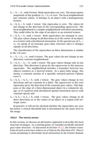
![232 10 Local Structure
because all we have to compute is the orientation of the line on which
the spectral densities are nonzero. Bigün and Granlund [2] devised the
following procedure:
• Use a window function to select a small local neighborhood from an
image;
• Fourier transform the windowed image. The smaller the selected
window, the more blurred the spectrum will be (uncertainty rela-
tion, see Section 3.2.3). This means that even with an ideal local
orientation we will obtain a rather band-shaped distribution of the
spectral energy; and
• Determine local orientation by fitting a straight line to the spectral
density distribution. This yields the angle of the local orientation
from the slope of the line.
The critical step of this procedure is fitting a straight line to the
spectral densities in the Fourier domain. We cannot solve this problem
exactly because it is generally overdetermined. When fitting a straight
line, we minimize the sum of the squares of the distances of the data
points to the line. This technique is known as the total least squares
approach
∞
d2 (k, r )|g(k)|2 dDk → min
¯ ˆ (10.59)
−∞
¯
The distance function is abbreviated using d(k, r ). The integral runs
over the whole wave number space; the wave numbers are weighted
with the spectral density |g(k)|2 . Equation (10.59) is not restricted to
ˆ
two dimensions, but is generally valid for local orientation or linear
symmetry in a D-dimensional space. The distance vector d is given by
T
¯ r
d = k − (k r )¯ (10.60)
The square of the distance is then given by
T T
|d|2 = |k − (k r )¯|2 = |k|2 − (k r )2
¯ r ¯ (10.61)
In order to express the distance more clearly as a function of the vector
¯
n, we rewrite it in the following manner
T T T
|d|2 = r (I(k k) − (kk ))¯
¯ r (10.62)
where I is the unit diagonal matrix. Substituting this expression into
Eq. (10.59) we obtain
r T J r → min
¯ ¯ (10.63)](https://image.slidesharecdn.com/computervision-handbookofcomputervisionandapplicationsvolume2-signalprocessingandpatternrecognition-120205081400-phpapp02/85/Computer-vision-handbook-of-computer-vision-and-applications-volume-2-signal-processing-and-pattern-recognition-257-320.jpg)
![10.6 First-order tensor representation 233
where J is a symmetric tensor with the diagonal elements
∞
Jr ,r = k2 |g(k)|2 dDk
s ˆ (10.64)
r ≠s−∞
and the off-diagonal elements
∞
Jr ,s = − kr ks |g(k)|2 dDk,
ˆ r ≠s (10.65)
−∞
The tensor J is analogous to a well-known physical quantity, the
inertia tensor . If we replace the wave number coordinates by space
coordinates and the spectral density |g(k)|2 by the specific density ρ,
ˆ
Eqs. (10.59) and (10.63) constitute the equation to compute the inertia
¯
of a rotary body rotating around the r axis.
With this analogy, we can reformulate the problem of determining
local orientation. We must find the axis about which the rotary body,
formed from the spectral density in Fourier space, rotates with mini-
mum inertia. This body might have different shapes. We can relate its
shape to the different solutions we get for the eigenvalues of the inertia
tensor and thus for the solution of the local orientation problem in 2-D:
Ideal local orientation. The rotary body is a line. For a rotation around
this line, the inertia vanishes. Consequently, the eigenvector to the
eigenvalue zero coincides with the direction of the line. The other
eigenvector is orthogonal to the line, and the corresponding eigen-
value is unequal to zero and gives the rotation axis for maximum
inertia;
Isotropic gray value. In this case, the rotary body is a kind of flat
isotropic disk. A preferred direction does not exist. Both eigenval-
ues are equal and the inertia is the same for rotations around all
axes. We cannot find a minimum; and
Constant gray values. The rotary body degenerates to a point at the
origin of the wave number space. The inertia is zero for rotation
around any axis. Therefore both eigenvalues vanish.
We derived the inertia tensor approach in the Fourier domain. Now
we will show how to compute the coefficients of the inertia tensor in
the spatial domain. The integrals in Eqs. (10.64) and (10.65) contain
terms of the form
k2 |g(k)|2 = |ikq g(k)|2
q ˆ ˆ
and
kp kq |g(k)|2 = ikp g(k)[ikq g(k)]∗
ˆ ˆ ˆ](https://image.slidesharecdn.com/computervision-handbookofcomputervisionandapplicationsvolume2-signalprocessingandpatternrecognition-120205081400-phpapp02/85/Computer-vision-handbook-of-computer-vision-and-applications-volume-2-signal-processing-and-pattern-recognition-258-320.jpg)
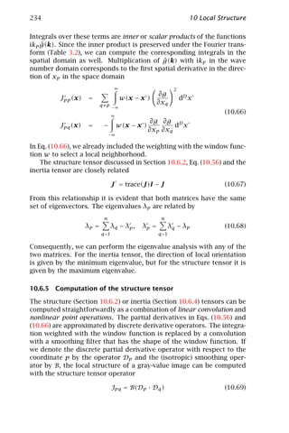
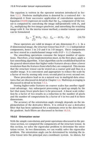
![236 10 Local Structure
example, by Jähne [4], the orientation angle is given by
2J12
tan 2φ = (10.71)
J22 − J11
Without defining any prerequisites, we have obtained the anticipated
angle doubling for orientation as discussed in Section 10.2.3 at the be-
ginning of this chapter. Since tan 2φ is gained from a quotient, we can
regard the dividend as the y and the divisor as the x component of a
vector and can form the orientation vector o, as introduced by Granlund
[1]
J22 − J11
o= (10.72)
2J12
The argument of this vector gives the orientation angle and the magni-
tude a certainty measure for local orientation.
The result of Eq. (10.72) is remarkable in that the computation of
the components of the orientation vector from the components of the
orientation tensor requires just one subtraction and one multiplication
by two. As these components of the orientation vector are all we need
for further processing steps, we do not need the orientation angle or the
magnitude of the vector. Thus, the solution of the eigenvalue problem
in two dimensions is trivial.
10.6.7 Coherency
The orientation vector reduces local structure to local orientation. From
three independent components of the symmetric tensor still only two
are used. When we fail to observe an orientated structure in a neighbor-
hood, we do not know whether any gray-value variations or distributed
orientations are encountered. This information is included in the not
yet used component of the tensor J11 + J22 , which gives the mean square
magnitude of the gradient. Consequently, a well-equipped structure
operator needs to include also the third component. A suitable linear
combination is
J11 + J22
s = J11 − J22 (10.73)
2J12
This structure operator contains the two components of the orientation
vector and, as an additional component, the mean square magnitude of
the gradient, which is a rotation-invariant parameter. Comparing the
latter with the magnitude of the orientation vector, a constant gray-
value area and an isotropic gray-value structure without preferred ori-
entation can be distinguished. In the first case, both squared quantities](https://image.slidesharecdn.com/computervision-handbookofcomputervisionandapplicationsvolume2-signalprocessingandpatternrecognition-120205081400-phpapp02/85/Computer-vision-handbook-of-computer-vision-and-applications-volume-2-signal-processing-and-pattern-recognition-261-320.jpg)
![238 10 Local Structure
10.7 References
[1] Granlund, G. H., (1978). In search of a general picture processing operator.
Comp. Graph. Imag. Process., 8:155–173.
[2] Bigün, J. and Granlund, G. H., (1987). Optimal orientation detection of
linear symmetry. In Proceedings ICCV’87, London 1987, pp. 433–438,
IEEE. Washington, DC: IEEE Computer Society Press.
[3] Granlund, G. H. and Knutsson, H., (1995). Signal Processing for Computer
Vision. Norwell, MA: Kluwer Academic Publishers.
[4] Jähne, B., (1997). Digital Image Processing—Concepts, Algorithms, and
Scientific Applications, 4th edition. New York: Springer.
[5] Kass, M. and Witkin, A., (1987). Analysing oriented patterns. Comp. Vis.
Graph. Im. Process., 37:362–385.
[6] Knutsson, H., (1989). Representing local structure using tensors. In The
6th Scandinavian Conference on Image Analysis, Oulu, Finland, June 19-
22, 1989.
[7] Rao, A. R. and Schunck, B. G., (1989). Computing oriented texture fields.
In Proceedings CVPR ’89, San Diego, CA, pp. 61–68, IEEE. Washington, DC:
IEEE Computer Society Press.
[8] Rao, A. R., (1990). A Taxonomy for Texture Description and Identification.
New York: Springer.
[9] Golub, G. H. and van Loan, C. F., (1989). Matrix Computations. Johns Hop-
kins Series in the Mathematical Sciences, No. 3. Baltimore: The Johns
Hopkins University Press.
[10] Hoffman, K. and Kunze, R., (1971). Linear Algebra, 2nd edition. Engle-
wood Cliffs, NJ: Prentice-Hall.
[11] Press, W. H., Flannery, B. P., Teukolsky, S. A., and Vetterling, W. T., (1992).
Numeral Recipes in C: the Art of Scientific Computing. New York: Cam-
bridge University Press.](https://image.slidesharecdn.com/computervision-handbookofcomputervisionandapplicationsvolume2-signalprocessingandpatternrecognition-120205081400-phpapp02/85/Computer-vision-handbook-of-computer-vision-and-applications-volume-2-signal-processing-and-pattern-recognition-263-320.jpg)
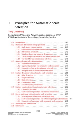
![240 11 Principles for Automatic Scale Selection
11.1 Introduction
An inherent property of objects in the world is that they only exist
as meaningful entities over certain ranges of scale. If one aims at de-
scribing the structure of unknown real-world signals, then a multiscale
representation of data is of crucial importance. Whereas conventional
scale-space theory provides a well-founded framework for dealing with
image structures at different scales, this theory does not directly ad-
dress the problem of how to select appropriate scales for further anal-
ysis.
This chapter outlines a systematic methodology for formulating
mechanisms for automatic scale selection in the domains of feature
detection and image matching.
11.2 Multiscale differential image geometry
A natural and powerful framework for representing image data at the
earliest stages of visual processing is by computing differential geomet-
ric image descriptors at multiple scales [1, 2]. This section summarizes
essential components of this scale-space theory [3], which also consti-
tutes the vocabulary for expressing the scale selection mechanisms.
11.2.1 Scale-space representation
Given any continuous signal g : RD → R, its linear scale-space represen-
tation L : RD × R+ → R is defined as the solution to the diffusion equation
D
1 2 1
∂t L = L= ∂xd xd L (11.1)
2 2
d =1
with initial condition L(x; 0) = g(x). Equivalently, this family can be
defined by convolution with Gaussian kernels h(x; t) of various width t
L(x; t) = h(x; t) ∗ g(x) (11.2)
where h : RD × R+ → R is given by
1 x 2 + . . . + xD
2
h(x, t) = exp − 1 (11.3)
(2π t)D/2 2t
and x = [x1 , . . . , xD ]T . There are several results [3, 4, 5, 6, 7, 8, 9,
10, 11, 12, 13, 14, 15, 16, 17, 18, 19] stating that within the class
of linear transformations the Gaussian kernel is the unique kernel for
generating a scale-space. The conditions that specify the uniqueness](https://image.slidesharecdn.com/computervision-handbookofcomputervisionandapplicationsvolume2-signalprocessingandpatternrecognition-120205081400-phpapp02/85/Computer-vision-handbook-of-computer-vision-and-applications-volume-2-signal-processing-and-pattern-recognition-265-320.jpg)
![11.2 Multiscale differential image geometry 241
are essentially linearity and shift invariance combined with different
ways of formalizing the notion that new structures should not be cre-
ated in the transformation from a finer to a coarser scale (see also
[18, 20, 21, 22, 23] for reviews).
11.2.2 Gaussian and directional derivative operators
From the scale-space representation, we can at any level of scale define
scale-space derivatives by
Lx α (x; t) = (∂x α L)(x; t) = ∂x α (h(x; t) ∗ g(x)) (11.4)
T
where α = [α1 , . . . , αD ] and ∂x α L = Lx1 α1 ...xD αD constitute multiindex
notation for the derivative operator ∂x α . Because differentiation com-
mutes with convolution, the scale-space derivatives can be written
Lx α (x; t) = (∂x α h(·; t)) ∗ g(x) (11.5)
and correspond to convolving the original image g with Gaussian deriva-
tive kernels ∂x α h. Figure 11.1 shows a few examples of such Gaussian
derivative operators.
The Gaussian derivatives provide a compact way to characterize the
local image structure around a certain image point at any scale. With
access to Gaussian derivative responses of all orders at one image point
x 0 , we can for any x in a neighborhood of x 0 reconstruct the original
scale-space representation by a local Taylor expansion. With θα denot-
ing the Taylor coefficient of order α, this reconstruction can be written
L(x; t) = θα Lx α (x 0 ; t) (x − x 0 )α (11.6)
α
Truncating this representation to derivatives up to order N, results in
a so-called N-jet representation [11].
The Gaussian derivatives according to Eq. (11.4) correspond to par-
tial derivatives along the Cartesian coordinate directions. Using the
n
well-known expression for the nth-order directional derivative ∂β of a
¯
function L in any direction β
n
∂β L = (cos β ∂x + sin β ∂y )n L
¯ (11.7)
we can express a directional derivative in any direction (cos β, sin β)
as a linear combination of the Cartesian Gaussian derivatives. (This
property is sometimes referred to as “steerability” [24, 25].) For orders
up to three, the explicit expressions are
∂β L
¯ = Lx cos β + Ly sin β
2
∂β L
¯ = Lxx cos2 β + 2Lxy cos β sin β + Lyy sin2 β
3
(11.8)
∂β L
¯ = Lxxx cos3 β + 3Lxxy cos2 β sin β
+ 3Lxyy cos β sin2 β + Lyyy sin3 β](https://image.slidesharecdn.com/computervision-handbookofcomputervisionandapplicationsvolume2-signalprocessingandpatternrecognition-120205081400-phpapp02/85/Computer-vision-handbook-of-computer-vision-and-applications-volume-2-signal-processing-and-pattern-recognition-266-320.jpg)
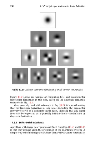
![244 11 Principles for Automatic Scale Selection
Another natural choice of a preferred coordinate system is to align
a local (p, q)-coordinate system to the eigenvectors of the Hessian ma-
trix. To express directional derivatives in such coordinates, character-
ized by the mixed second-order derivative Lpq being zero, we can rotate
the coordinate system by an angle ψ defined by
1 Lxx −Lyy
cos ψ (x0 ,y0 ) = 1+
2 (Lxx −Lyy )2 +4L2
xy
(x0 ,y0 )
(11.12)
1 Lxx −Lyy
sin ψ (x0 ,y0 ) = (sgn Lxy ) 1−
2 (Lxx −Lyy )2 +4L2
xy
(x0 ,y0 )
and define unit vectors in the p- and q-directions by ep = (sin ψ, − cos ψ)
and eq = (cos ψ, sin ψ) with associated directional derivative operators
∂p = sin ψ ∂x − cos ψ ∂y , ∂q = cos ψ ∂x + sin ψ ∂y (11.13)
Then, it is straightforward to verify that this definition implies that
Lpq = ∂p ∂q L = (cos ψ ∂x + sin ψ ∂y ) (sin ψ ∂x − cos ψ ∂y )L
(11.14)
= cos ψ sin ψ (Lxx − Lyy ) − (cos2 ψ − sin2 ψ) Lxy = 0
A more general class of (nonlinear) differential invariants will be con-
sidered in Section 11.3.2.
11.2.4 Windowed spectral moment descriptors
The differential invariants defined so far depend upon the local differ-
ential geometry at any given image point. One way of defining regional
image descriptors, which reflect the intensity distribution over image
patches, is by considering windowed spectral moment descriptors (see
also [3, 26, 27]). Using Plancherel’s relation
ˆ ˆ∗
f1 (ω) f2 (ω) dω = (2π )2 ∗
f1 (x) f2 (x) dx (11.15)
ω∈R 2 x ∈R 2
ˆ
where hi (ω) denotes the Fourier transform of hi (x) (with ω = 2π k as
variable in the frequency domain) and by letting f1 = Lx α and f2 = Lx β ,
we have
ˆ
(iω)|α|+|β| |L|2 (ω) dω = (2π )2 Lx α (x) Lx β (x) dx (11.16)
ω∈R 2 x ∈ R2
Let us next introduce a Gaussian window function h(·; s), depending
on an integration scale parameter s, in addition to the local scale pa-
rameter t of the ordinary scale-space representation. Then, we can](https://image.slidesharecdn.com/computervision-handbookofcomputervisionandapplicationsvolume2-signalprocessingandpatternrecognition-120205081400-phpapp02/85/Computer-vision-handbook-of-computer-vision-and-applications-volume-2-signal-processing-and-pattern-recognition-269-320.jpg)
![11.2 Multiscale differential image geometry 245
define the following windowed spectral moments:
µ20 (x; t, s) = L2 (ξ; t) h(x − ξ; s) dξ,
x
ξ ∈ R2
µ11 (x; t, s) = Lx (ξ; t) Ly (ξ; t) h(x − ξ; s) dξ, (11.17)
ξ ∈ R2
µ02 (x; t, s) = L2 (ξ; t) h(x − ξ; s) dξ
y
ξ ∈ R2
and higher-order spectral moment descriptors can be defined in an
analogous fashion.
11.2.5 The scale-space framework for a visual front-end
The image descriptors defined in Section 11.2.2 to Section 11.2.4 pro-
vide a useful basis for expressing a large number of early visual opera-
tions, including image representation, feature detection, stereo match-
ing, optic flow and shape estimation. There is also a close connection
to biological vision. Neurophysiological studies by Young [28, 29] have
shown that there are receptive fields in the mammalian retina and vi-
sual cortex, which can be well modeled by Gaussian derivatives up to
order four. In these respects, the scale-space representation with its
associated Gaussian derivative operators can be seen as a canonical
idealized model of a visual front-end.
When computing these descriptors at multiple scales, however, as
is necessary to capture the complex multiscale nature of our world,
one can expect these descriptors to accurately reflect interesting image
structures at certain scales, while the responses may be less useful
at other scales. To simplify the interpretation tasks of later processing
stages, a key problem of a visual front-end (in addition to making image
structures more explicit by computing differential image descriptors
at multiple scales) is to provide hypothesis about how to select locally
appropriate scales for describing the data set.
11.2.6 The need for automatic scale selection
To illustrate the need for an explicit mechanism for automatic scale
selection, let us first consider the problem of detecting edges. The
left column in Fig. 11.3 shows the result of applying a standard edge
detector (described in Section 11.4.1) to an image, which have been
smoothed by convolution with Gaussian kernels of different widths.
As can be seen, different types of edge structures give rise to edge
curves at different scales. For example, the shadow of the arm only
appears as a connected edge curve at coarse scales. If such coarse scales
are used at the finger tip, however, the shape distortions due to scale-
space smoothing will be substantial. Hence, to extract this edge with](https://image.slidesharecdn.com/computervision-handbookofcomputervisionandapplicationsvolume2-signalprocessingandpatternrecognition-120205081400-phpapp02/85/Computer-vision-handbook-of-computer-vision-and-applications-volume-2-signal-processing-and-pattern-recognition-270-320.jpg)
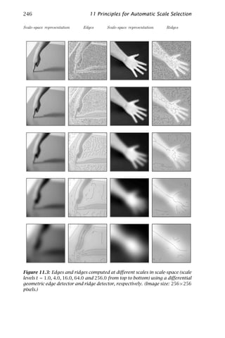
![11.3 A general scale-selection principle 247
a reasonable trade-off between detection and localization properties,
the only reasonable choice is to allow the scale levels to vary along the
edge.
The right column in Fig. 11.3 shows corresponding results for a
ridge detector (described in Section 11.4.2). Different types of ridge
structures give rise to qualitatively different types of ridge curves de-
pending on the scale level. The fingers respond at t ≈ 16, whereas the
arm as a whole is extracted as a long ridge curve at t ≈ 256.
For these reasons, and because the choice of scale levels crucially
affects the performance of any feature detector, and different scale
levels will, in general, be required in different parts of the image, it is
essential to complement feature detectors by explicit mechanisms that
automatically adapt the scale levels to the local image structure.
11.3 A general scale-selection principle
A powerful approach to perform local and adaptive scale selection is by
detecting local extrema over scales of normalized differential entities.
This chapter presents a general theory by first introducing the notion
of normalized derivatives, and then showing how local extrema over
scales of normalized differential entities reflect the characteristic size
of corresponding image structures.
11.3.1 Normalized derivatives and intuitive idea for scale selec-
tion
A well-known property of the scale-space representation is that the
amplitude of spatial derivatives
Lx α (·; t) = ∂x α L(·; t) = ∂x α1 . . . ∂x αD L(·; t)
1 D
in general decrease with scale, that is, if a signal is subject to scale-space
smoothing, then the numerical values of spatial derivatives computed
from the smoothed data can be expected to decrease. This is a direct
consequence of the nonenhancement property of local extrema, which
means that the value at a local maximum cannot increase, and the value
at a local minimum cannot decrease [3, 4]. In other words, the ampli-
tude of the variations in a signal will always decrease with scale.
As a simple example of this, consider a sinusoidal input signal of
some given angular frequency ω0 = 2π k0 ; for simplicity, in one dimen-
sion
g(x) = sin ω0 x (11.18)](https://image.slidesharecdn.com/computervision-handbookofcomputervisionandapplicationsvolume2-signalprocessingandpatternrecognition-120205081400-phpapp02/85/Computer-vision-handbook-of-computer-vision-and-applications-volume-2-signal-processing-and-pattern-recognition-272-320.jpg)
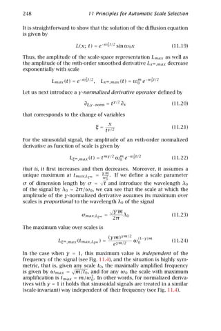
![11.3 A general scale-selection principle 249
Lx ;max (t)
0.6
0.5 w 1 = 0.5
0.4
0.3
0.2
0.1
w 3 = 2.0 w 2 = 1.0
0
0 2 4 6 8 10 scale t
Figure 11.4: The amplitude of first-order normalized derivatives as function
of scale for sinusoidal input signals of different frequency (ω1 = 0.5, ω2 = 1.0
and ω3 = 2.0).
11.3.2 A general principle for automatic scale selection
The example shows that the scale at which a normalized derivative as-
sumes its maximum over scales is for a sinusoidal signal proportional
to the wavelength of the signal. In this respect, maxima over scales of
normalized derivatives reflect the scales over which spatial variations
take place in the signal. This property is, however, not restricted to
sine wave patterns or to image measurements in terms of linear deriva-
tive operators of a certain order. On the contrary, it applies to a large
class of image descriptors that can be formulated as multiscale differ-
ential invariants expressed in terms of Gaussian derivatives. In [3], the
following scale selection principle was proposed:
In the absence of other evidence, assume that a scale level, at
which some (possibly nonlinear) combination of normalized deriva-
tives assumes a local maximum over scales, can be treated as re-
flecting a characteristic length of a corresponding structure in the
data.
11.3.3 Properties of the scale-selection principle
A basic justification for the forementioned statement can be obtained
from the fact that for a large class of (possibly nonlinear) combinations
of normalized derivatives it holds that maxima over scales exhibit de-
sirable behavior under rescalings of the intensity pattern. If the input
image is rescaled by a constant scaling factor s, then the scale at which
the maximum is assumed will be multiplied by the same factor (if mea-
√
sured in units of σ = t). This is a fundamental requirement on a scale
selection mechanism, as it guarantees that image operations commute
with size variations.](https://image.slidesharecdn.com/computervision-handbookofcomputervisionandapplicationsvolume2-signalprocessingandpatternrecognition-120205081400-phpapp02/85/Computer-vision-handbook-of-computer-vision-and-applications-volume-2-signal-processing-and-pattern-recognition-274-320.jpg)
![250 11 Principles for Automatic Scale Selection
Scaling properties. For two signals g and g related by
g(x) = g (sx) (11.25)
the corresponding normalized derivatives defined from the scale-space
representations L and L on the two domains are related according to
∂ξ m L(x; t) = s m(1−γ) ∂ξ m L (x ; t ) (11.26)
and when γ = 1, the normalized derivatives are equal at corresponding
points (x; t) and (x ; t ) = (sx; s 2 t).
When γ ≠ 1, a weaker scale-invariance properties holds. Let us
consider a homogeneous polynomial differential invariant DL of the
form
I J J
DL = ci Lx αij with |αij | = M (11.27)
i=1 j =1 j =1
The sum of the orders of differentiation in the last term does not de-
pend on the index i of that term. Then, normalized differential expres-
sions in the two domains are related by
Dγ −norm L = s M(1−γ) Dγ −norm L (11.28)
that is, magnitude measures scale according to a power law. Local max-
ima over scales are, however, still preserved
∂t Dγ −norm L = 0 ∂t Dγ −norm L =0 (11.29)
that gives sufficient scale invariance to support the scale selection meth-
odology. More generally, it can be shown that the notion of γ-normal-
ized derivatives arises by necessity, given natural requirements of a
scale-selection mechanism [30].
11.3.4 Interpretation of normalized derivatives
Lp -norms. For a D-dimensional signal, it can be shown that the varia-
tion over scales of the Lp -norm of an mth-order normalized Gaussian
derivative kernel is given by
m(γ −1)+D(1/p −1)
hξ m (·; t) p = t hξ m (·; t) p (11.30)
In other words, the Lp -norm of the mth-order Gaussian derivative ker-
nel is constant over scales if and only if
1
p= m (11.31)
1+ D (1 − γ)](https://image.slidesharecdn.com/computervision-handbookofcomputervisionandapplicationsvolume2-signalprocessingandpatternrecognition-120205081400-phpapp02/85/Computer-vision-handbook-of-computer-vision-and-applications-volume-2-signal-processing-and-pattern-recognition-275-320.jpg)
![11.4 Feature detection with automatic scale selection 251
Hence, the γ-normalized derivative concept be interpreted as an Lp -
normalization of the Gaussian derivative kernels over scales for a spe-
cific value of p, which depends upon γ, the dimension as well as the
order m of differentiation. The perfectly scale-invariant case γ = 1
gives p = 1 for all orders m and corresponds to L1 -normalization of
the Gaussian derivative kernels.
Power spectra. For a signal g : R2 → R having a power spectrum of
the form
ˆˆ
Sg (ω1 , ω2 ) = (f f ∗ )(ω1 , ω2 ) = |ω|−2α = (ω2 + ω2 )−α (11.32)
1 2
it can be shown that the variation over scales of the following energy
measure:
PL(·; t) = | L(x; t)|2 dx (11.33)
x ∈ R2
is given by
Pnorm (·; t) = t γ PL(·; t) ∼ t α+γ −2 (11.34)
This expression is independent of scale if and only if α = 2 − γ. In other
words, in the 2-D case the normalized derivative model is neutral with
respect to power spectra of the form Sg (ω) = |ω|−2(2−γ) (and natural
images often have power spectra of this form [31]).
11.4 Feature detection with automatic scale selection
This section shows how the general principle for automatic scale selec-
tion described in Section 11.3.2 can be integrated with various types of
feature detectors.
11.4.1 Edge detection
At any scale in scale-space, let us define an edge point as a point at
which the second directional derivative Lvv in the v-direction is zero,
and the third directional derivative Lvvv is negative
Lvv = 0,
(11.35)
Lvvv < 0
The edges in Fig. 11.3 have been computed according to this definition
[3, 32, 33, 34].
In view of the scale-selection principle, a natural extension of this
notion of nonmaximum suppression is by defining a scale-space edge a](https://image.slidesharecdn.com/computervision-handbookofcomputervisionandapplicationsvolume2-signalprocessingandpatternrecognition-120205081400-phpapp02/85/Computer-vision-handbook-of-computer-vision-and-applications-volume-2-signal-processing-and-pattern-recognition-276-320.jpg)
![252 11 Principles for Automatic Scale Selection
curve on this edge surface, such that some measure of edge strength
Eγ −norm L assumes locally maxima with respect to scale on this curve
∂t (Eγ −norm L(x, y; t)) = 0,
∂ (E
tt γ −norm L(x, y; t)) < 0,
(11.36)
Lvv (x, y; t) = 0,
L
vvv (x, y; t) < 0
Based on the γ-parameterized normalized derivative concept, we shall
here consider the following two edge strength measures:
Gγ −norm L = t γ L2
v and Tγ −norm L = −t 3 γ L3 Lvvv
v (11.37)
Qualitative properties. For a diffuse step edge, defined as the primi-
tive function of a 1-D Gaussian
x
ft0 (x, y) = h(x ; t0 ) dx
x =−∞
each of these edge strength measures assumes a unique maximum over
scales at tGγ −norm = tTγ −norm = (γ/(1 − γ))t0 . Requiring this maximum to
occur at t0 gives γ = 1/2.
For a local model of an edge bifurcation, expressed as
L(x; t) = 1 x 4 + 3 x 2 (t − tb ) + 3 (t − tb )2
4 2 4 (11.38)
with edges at x1 (t) = (tb − t)1/2 when t ≤ tb , we have
(Gγ −norm L)(x1 (t); t) = 4 t γ (tb − t)3 (11.39)
and the selected scales are
γ 3γ
tGγ −norm = tb and tTγ −norm = tb (11.40)
3+γ 5 + 3γ
In other words, the scale selection method has the qualitative property
of reflecting the degree of diffuseness of the edge. Moreover, as the edge
strength decreases rapidly at a bifurcation, the selected scales will tend
away from bifurcation scales.
Results of edge detection. Let us now apply the integrated edge de-
tection scheme to different real-world images. In brief, edges are ex-
tracted as follows [35]: The differential descriptors in the edge defini-
tion, (11.36) are rewritten in terms of partial derivatives in Cartesian
coordinates and are computed at a number of scales in scale-space.
Then, a polygon approximation is constructed of the intersections of
the two zero-crossing surfaces of Lvv and ∂t (Eγ −norm ) that satisfy the
sign conditions Lvvv < 0 and ∂t (Eγ −norm ) < 0. Finally, a significance](https://image.slidesharecdn.com/computervision-handbookofcomputervisionandapplicationsvolume2-signalprocessingandpatternrecognition-120205081400-phpapp02/85/Computer-vision-handbook-of-computer-vision-and-applications-volume-2-signal-processing-and-pattern-recognition-277-320.jpg)
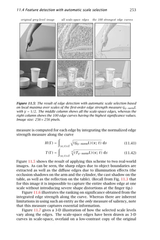
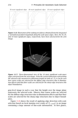
![11.4 Feature detection with automatic scale selection 255
original grey-level image the 1000 most salient scale-space edges
Figure 11.8: The 1000 strongest scale-space edges extracted using scale selec-
tion based on local maxima over scales of Tγ −norm L (with γ = 1/2). (Image size:
256 × 256 pixels.)
these results may appear very similar to the result of traditional edge
detection at a fixed (very fine) scale. A more detailed study, however,
reveals that a number of shadow edges are extracted, which would be
impossible to detect at the same scale as the dominant fine-scale in-
formation. In this context, it should be noted that the fine-scale edge
detection in this case is not the result of any manual setting of tuning
parameters. It is a direct consequence of the scale-space edge concept,
and is the result of applying the same mechanism as extracts coarse
scale levels for diffuse image structures.
Summary. To conclude, for both these measures of edge strength, this
scale selection scheme has the desirable property of adapting the scale
levels to the local image structure such that the selected scales reflect
the degree of diffuseness of the edge.
11.4.2 Ridge detection
By a slight reformulation, ridge detection algorithms can be expressed
in a similar way. If we follow a differential geometric approach, and
define a bright (dark) ridge point as a point for which the brightness
assumes a maximum (minimum) in the main eigendirection of the Hes-
sian matrix [20, 36, 37, 38], then in the (p, q)-system this definition can
be stated as
Lp = 0,
Lq = 0,
Lpp < 0, or Lqq < 0,
|Lpp | ≥ |Lqq | |Lqq | ≥ |Lpp |](https://image.slidesharecdn.com/computervision-handbookofcomputervisionandapplicationsvolume2-signalprocessingandpatternrecognition-120205081400-phpapp02/85/Computer-vision-handbook-of-computer-vision-and-applications-volume-2-signal-processing-and-pattern-recognition-280-320.jpg)
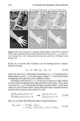
![11.4 Feature detection with automatic scale selection 257
backprojection of ridge 1 backprojection of ridges 2–5
Figure 11.10: Alternative illustration of the five strongest scale-space ridges
extracted from the image of the arm in Fig. 11.9. Each ridge is backprojected
onto a dark copy of the original image as the union of a set of circles centered on
the ridge curve with the radius proportional to the selected scale at that point.
Qualitative properties. For a Gaussian ridge defined by g(x, y) =
h(x; t0 ), it can be shown that the selected scale will then be tRγ −norm =
2γ
3− 2 γ t0 . Requiring this scale to be tRγ −norm = t0 , gives γ = 3 .
4
Results of ridge detection. Figure 11.9 shows the result of apply-
ing such a ridge detector to two images and selecting the 100 and
10 strongest bright ridges, respectively, by integrating a measure of
normalized ridge strength along each curve. For the arm image, ob-
serve how a coarse-scale descriptor is extracted for the arm as a whole,
whereas the individual fingers give rise to ridge curves at finer scales
(see also Fig. 11.10).
11.4.3 Blob detection
The Laplacian operator 2 L = Lxx + Lyy is a commonly used entity for
blob detection, because it gives a strong response at the center of blob-
like image structures [39, 40, 41]. To formulate a blob detector with
automatic scale selection, we can consider the points in scale-space at
which the the square of the normalized Laplacian
2
norm L = t(Lxx + Lyy ) (11.46)
assumes maxima with respect to space and scale. Such points are re-
ferred to as scale-space extrema of ( 2 2
norm L) .
Qualitative properties. For a Gaussian blob defined by
1 2 2
g(x, y) = h(x, y; t0 ) = e−(x +y )/2t0 (11.47)
2π t0](https://image.slidesharecdn.com/computervision-handbookofcomputervisionandapplicationsvolume2-signalprocessingandpatternrecognition-120205081400-phpapp02/85/Computer-vision-handbook-of-computer-vision-and-applications-volume-2-signal-processing-and-pattern-recognition-282-320.jpg)
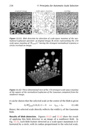
![11.4 Feature detection with automatic scale selection 259
Figure 11.12 shows a 3-D illustration of the same data set, by mark-
ing the scale-space extrema by spheres in scale-space. Observe how
the size variations in the image are captured by this structurally very
simple operation.
11.4.4 Corner detection
A commonly used technique for detecting junction candidates in gray-
level images is to detect extrema in the curvature of level curves mul-
tiplied by the gradient magnitude raised to some power [42, 43]. A
special choice is to multiply the level curve curvature by the gradient
magnitude raised to the power of three. This leads to the differential
invariant κ = L2 Luu , with the corresponding normalized expression
˜ v
κnorm = t 2γ L2 Luu
˜ v (11.49)
Qualitative properties. For a diffuse L-junction
g(x1 , x2 ) = Φ(x1 ; t0 ) Φ(x2 ; t0 ) (11.50)
modeled as the product of two diffuse step edges
xi
Φ(xi ; t0 ) = h(x ; t0 ) dx (11.51)
x =−∞
˜
it can be shown that variation of κnorm at the origin is given by
t 2γ
˜
|κnorm (0, 0; t)| = (11.52)
8π 2 (t0 + t)2
When γ = 1, this entity increases monotonically with scale, whereas
˜
for γ ∈]0, 1[, κnorm (0, 0; t) assumes a unique maximum over scales
γ
at tκ = 1−γ t0 . On the other hand, for a nonuniform Gaussian blob
˜
L(x1 , x2 ; t) = h(x1 ; t1 + t) h(x2 ; t2 + t), the normalized response
always decreases with scale at sufficiently coarse scales.
˜2
This analysis indicates that when γ = 1, κnorm can be expected to
increase with scales when a single corner model of infinite extent con-
˜2
stitutes a reasonable approximation, whereas κnorm can be expected
to decrease with scales when so much smoothing is applied that the
overall shape of the object is substantially distorted.
˜2
Hence, selecting scale levels (and spatial points) where κnorm as-
sumes maxima over scales can be expected to give rise to scale levels
in the intermediate scale range (where a finite extent junction model
constitutes a reasonable approximation) and the selected scale levels
thus reflect over how large a region a corner model is valid. In practice,
a slightly smaller value of γ = 7/8 is used.](https://image.slidesharecdn.com/computervision-handbookofcomputervisionandapplicationsvolume2-signalprocessingandpatternrecognition-120205081400-phpapp02/85/Computer-vision-handbook-of-computer-vision-and-applications-volume-2-signal-processing-and-pattern-recognition-284-320.jpg)
![260 11 Principles for Automatic Scale Selection
˜2
Figure 11.13: Three-dimensional view of scale-space maxima of κnorm com-
puted for a large scale corner with superimposed corner structures at finer
scales.
Results of corner detection. Figure 11.13 shows the result of detect-
ing scale-space extrema from an image with corner structures at mul-
tiple scales. Observe that a coarse scale response is obtained for the
large-scale corner structure as a whole, whereas the superimposed cor-
ner structures of smaller size give rise to scale-space maxima at finer
scales. (More results on real images will be shown in Section 11.5.)
11.4.5 Local frequency estimation
To extend the forementioned application of the scale selection method-
ology from the detection of sparse image features to the computation
of dense image descriptors, a natural starting point is to consider the
theory of quadrature filter pairs defined (from a Hilbert transform) in
such a way as to be phase-independent for any sine wave. To approxi-
mate such operators within the Gaussian derivative framework, we can
define a corresponding quasi-quadrature measure in the 1-D case by
[11, 44]
P L = L2 + CL2 = tL2 + Ct 2 L2
ξ ξξ x xx (11.53)
where a good choice of the parameter C is C = e/4. Note that, in order
to achieve scale invariance, it is necessary to use normalized deriva-
tives with γ = 1 in the (inhomogeneous) linear combination of Gaussian
derivatives of different order. The γ-normalized derivative concept,
however, leaves a degree of freedom, which can be parameterized by
P L = t −Γ (tL2 + Ct 2 L2 )
x xx (11.54)](https://image.slidesharecdn.com/computervision-handbookofcomputervisionandapplicationsvolume2-signalprocessingandpatternrecognition-120205081400-phpapp02/85/Computer-vision-handbook-of-computer-vision-and-applications-volume-2-signal-processing-and-pattern-recognition-285-320.jpg)
![11.4 Feature detection with automatic scale selection 261
2000
1000
PnormL
0
−1000
−2000
120
100
80 6
60 4
40 2
20 0
−2
space (y) effective scale (log_2 t)
Figure 11.14: Dense scale selection by maximizing the quasi-quadrature mea-
sure Eq. (11.55) over scales: (left) original gray-level image; (right) the variations
over scales of the quasi-quadrature measure P L computed along a vertical cross
section through the center of the image. The result is visualized as a surface
plot showing the variations over scale of the quasi-quadrature measure as well
as the position of the first local maximum over scales.
To extend this entity to 2-D signals, we can consider
P L = t −Γ t(L2 + L2 ) + C t 2 (L2 + 2L2 + L2 )
x y xx xy yy (11.55)
RL = t −Γ t (L2 + L2 ) + C t 2 ((Lxx − Lyy )2 + 4 L2 )
x y xy (11.56)
Both these differential expressions are invariant under rotations and
reduce to the form of Eq. (11.54) for a 1-D signal. The second-order
differential expression in Eq. (11.55)
Sγ −nor m L = t 2 γ (L2 + 2L2 + L2 )
xx xy yy (11.57)
however, is a natural measure of the total amount of second-order infor-
mation in the signal, whereas the second-order differential expression
in (Eq. (11.56))
Aγ −norm L = t 2 γ (Lpp − Lqq )2 = t 2 γ ((Lxx − Lyy )2 + 4 L2 )
xy (11.58)
is more specific to elongated structures (e.g., ridges). The specific choice
of Γ = 1/2 means that Eq. (11.56) and can be interpreted as a linear com-
bination of the edge strength measure Eq. (11.37) with γ = 1/2 and the
ridge strength measure (Eq. (11.58)) with γ = 3/4.
Qualitative properties. These differential expressions inherit simi-
lar scale selection properties for sine waves as those described in Sec-
tion 11.3.1; see [30, 44] for an analysis.](https://image.slidesharecdn.com/computervision-handbookofcomputervisionandapplicationsvolume2-signalprocessingandpatternrecognition-120205081400-phpapp02/85/Computer-vision-handbook-of-computer-vision-and-applications-volume-2-signal-processing-and-pattern-recognition-286-320.jpg)
![262 11 Principles for Automatic Scale Selection
Results of frequency estimation. Figure 11.14 shows an example re-
sult of estimating local frequencies in this way, by detecting local max-
ima over scale of P L along a vertical cross section in an image of a
periodic pattern. Observe how the selected scale levels capture the
variations in frequency caused by the perspective effects.
11.5 Feature localization with automatic scale selection
The scale-selection techniques presented so far are useful in the stage
of detecting image features. The role of the scale-selection mechanism
is to estimate the approximate size of the image structures to which the
feature detector responds. When computing features at coarse scales
in scale-space, however, the shape distortions can be significant, and
in many cases it is desirable to complement feature-detection modules
by an explicit feature-localization stage.
The goal of this section is to show how the mechanism for auto-
matic scale selection can be formulated in this context by minimizing
measures of inconsistency over scales.
11.5.1 Corner localization
Given an approximate estimate x0 of the location and the size s of a
corner (computed according to Section 11.4.4), an improved estimate
of the corner position can be computed as follows [3, 45]: Consider at
every point x ∈ R2 in a neighborhood of x0 , the line lx perpendicular
to the gradient vector ( L)(x ) = (Lx1 , Lx2 )T (x ) at that point
Dx (x) = (( L)(x ))T (x − x ) = 0 (11.59)
Then, minimize the perpendicular distance to all lines lx in a neigh-
borhood of x0 , weighted by the gradient magnitude, that is, determine
the point x ∈ R2 that minimizes
2
min (Dx (x)) wx0 (x ; s) dx (11.60)
x ∈ R2 x ∈R 2
for a Gaussian window function wx0 (·; s) : R2 → R with integration
scale s set from the detection scale ttildeκ of the corner and centered at
the candidate junction x0 . After expansion, this minimization problem
can be expressed as a standard least squares problem
min x T A x − 2 x T b + c ⇐⇒ Ax = b (11.61)
x ∈ R2
where x = (x1 , x2 )T , and A, b, and c are determined by the local statis-
tics of the gradient directions L(·; t) at scale t in a neighborhood of](https://image.slidesharecdn.com/computervision-handbookofcomputervisionandapplicationsvolume2-signalprocessingandpatternrecognition-120205081400-phpapp02/85/Computer-vision-handbook-of-computer-vision-and-applications-volume-2-signal-processing-and-pattern-recognition-287-320.jpg)
![11.5 Feature localization with automatic scale selection 263
T -junction (t0 = 0.0) ˜
signature dmin estimated position
50
40
30
noise 1.0
20
10
0
0 1 2 3 4 5 6
160
140
120
100
noise 30.0 80
60
40
20
0
0 1 2 3 4 5 6
Figure 11.15: Corner localization by minimizing the normalized residuals over
scales for two corner structures. A basic property of the scale-selection mecha-
nism is that an increase in the noise level implies that the minimum over scales
is assumed at a coarser scale.
x0 (compare with Eq. (11.17))
A(x; t, s) = ( L)(x ) ( L)T (x ) wx0 (x ; s) dx (11.62)
x ∈ R2
b(x; t, s) = ( L)(x ) ( L)T (x ) x wx0 (x ; s) dx (11.63)
x ∈ R2
T
c(x; t, s) = x ( L)(x ) ( L)T (x ) x wx0 (x ; s) dx (11.64)
x ∈ R2
11.5.2 Scale-selection principle for feature localization
To express a scale-selection mechanism for this corner localizer, let us
extend the minimization problem (Eq. (11.61)) from a single scale to
optimization over multiple scales [46]
xT A x − 2 xT b + c c − b T A− 1 b
min min = min min (11.65)
t ∈ R+ x ∈ R 2 norm(t) t ∈ R+ x ∈ R 2 trace A
and introduce a normalization factor norm(t) to relate minimizations
at different scales. The particular choice of norm(t) = trace A implies
that the normalized residual
2
x ∈ R2 (( L)(x ))T (x − x ) wx0 (x ; s) dx
˜
r = min 2
(11.66)
x ∈ R2
x ∈ R2 ( L)(x ) wx0 (x ; s) dx](https://image.slidesharecdn.com/computervision-handbookofcomputervisionandapplicationsvolume2-signalprocessingandpatternrecognition-120205081400-phpapp02/85/Computer-vision-handbook-of-computer-vision-and-applications-volume-2-signal-processing-and-pattern-recognition-288-320.jpg)
![264 11 Principles for Automatic Scale Selection
original image 100 strongest junctions
Figure 11.16: Results of composed two-stage junction detection followed by
junction localization. (left) Original gray-level image. (right) The 100 strongest
˜2
junction responses ranked according to the scale-space maxima of κnorm and
illustrated by circles with their radii proportional to the detection scales of the
junction responses.
has dimension [length]2 that can be interpreted as a weighted esti-
mate of the localization error. Specifically, scale selection according to
˜
Eq. (11.65), by minimizing the normalized residual r of Eq. (11.66) over
scales, corresponds to selecting the scale that minimizes the estimated
inaccuracy in the localization estimate.
Qualitative effects. Figure 11.15 shows the result of performing cor-
ner localization in this way, by minimizing the normalized residual r ˜
over scales for two corner structures. Observe how an increase in the
noise level implies that the minimum over scales is assumed at a coarser
scale.
Results of corner localization. Figure 11.16 shows the result of in-
tegrating this corner localization module with the corner detector in
Section 11.4.4. The resulting two-stage corner automatically adapts
its detection scales and localization scales to size variations and noise
variations in the image structures. In addition, the region of interest
associated with each corner is useful for purposes such as matching.
Edge localization. In Lindeberg [3, 30] it is outlined how minimization
over scales of a similar normalized residual applies to the problem of
edge localization.](https://image.slidesharecdn.com/computervision-handbookofcomputervisionandapplicationsvolume2-signalprocessingandpatternrecognition-120205081400-phpapp02/85/Computer-vision-handbook-of-computer-vision-and-applications-volume-2-signal-processing-and-pattern-recognition-289-320.jpg)
![11.6 Stereo matching with automatic scale selection 265
11.6 Stereo matching with automatic scale selection
This section shows how a scale selection mechanism can be formu-
lated for a differential stereo matching scheme expressed within the
Gaussian derivative framework. With appropriate modifications, simi-
lar ideas apply to the problem of flow estimation.
11.6.1 Least squares differential stereo matching
Let us assume that the flow field between the scale-space representa-
tions L and R of two images can be approximated by a constant flow
field v over the support region of a window function w. Following
[47, 48, 49, 50, 51] and several others, consider the discrete form of
the motion constraint equation [52]
( L)(ξ)T (∆ξ) + (L(ξ) − R(ξ)) = O(|∆ξ |2 ) (11.67)
and integrate the square of this relation using w as window function.
After expansion (and dropping the arguments) this gives the least-
squares problem
min v T Av + 2bT v + c (11.68)
v ∈R 2
where A, b, and c are defined by
A= ( L)( L)T w dξ
ξ ∈ R2
(11.69)
b= (R − L) ( L) w dξ, c= (R − L)2 w dξ
ξ ∈R 2 ξ ∈ R2
If we interpret R − L as a discrete approximation to a temporal deriva-
tive, these image descriptors fall within the class of windowed spectral
moments in Eq. (11.17). Assuming that A according to Eq. (11.69) is
nondegenerate, the explicit solution of the flow estimate is
v = −A−1 b (11.70)
11.6.2 Scale-selection principle for estimating image deformations
When implementing this scheme in practice, it is natural to express it
within a coarse-to-fine multiscale framework. When performing image
matching from coarse to fine scales, however, it is not obvious what
should be the finest scales. If we attempt to match image features be-
yond a certain resolution, we could expect the errors in the deformation
estimates to increase rather than to decrease.
In analogy with Section 11.5.2, a natural way to formulate a scale-
selection mechanism for the differential stereo matching scheme is by](https://image.slidesharecdn.com/computervision-handbookofcomputervisionandapplicationsvolume2-signalprocessingandpatternrecognition-120205081400-phpapp02/85/Computer-vision-handbook-of-computer-vision-and-applications-volume-2-signal-processing-and-pattern-recognition-290-320.jpg)
![266 11 Principles for Automatic Scale Selection
first image second image ˜
signature of r
size: 4
size: 16
˜
Figure 11.17: Scale-space signatures of the normalized residual r for synthetic
expanding patterns with structures at different scales. Notice that with increas-
ing size of the texture elements, the minimum over scales in the normalized
residual is assumed at coarser scales.
extending the least squares estimation (Eq. (11.68)) to the two-parameter
least squares problem
v T Av + 2bT v + c
min min (11.71)
t ∈R + v ∈R 2 norm(t)
where the normalization factor norm(t) determines how the informa-
tion at different scales should be compared. Again, we choose norm(t) =
trace A, while one could also conceive other normalization approaches,
such as the minimum eigenvalue of A.
The resulting normalized residual is of dimension [length]2 and
constitutes a first-order approximation of the following error measure:
ξ ∈R 2 |( L)T (v − ∆ξ)|2 w(ξ) dξ
E L =
ξ ∈R 2 | L|2 w(ξ) dξ
ξ ∈R2 (v − ∆ξ)T ( L)( L)T (v − ∆ξ) w(ξ) dξ
= (11.72)
ξ ∈R 2 ( L)T ( L) w(ξ) dξ
where v is the regional flow estimate and ∆ξ a pointwise flow estimate
that satisfies Eq. (11.67). In other words, E L can be seen as a measure
of the internal consistency of the estimated flow field, weighted by the
gradient magnitude.](https://image.slidesharecdn.com/computervision-handbookofcomputervisionandapplicationsvolume2-signalprocessingandpatternrecognition-120205081400-phpapp02/85/Computer-vision-handbook-of-computer-vision-and-applications-volume-2-signal-processing-and-pattern-recognition-291-320.jpg)
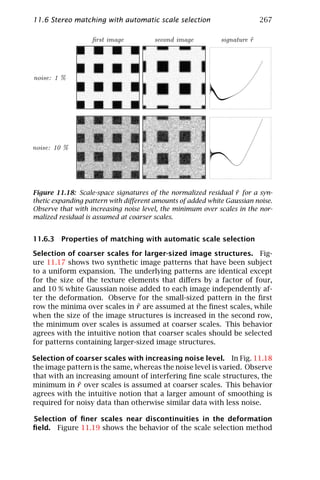
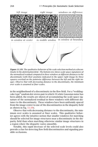
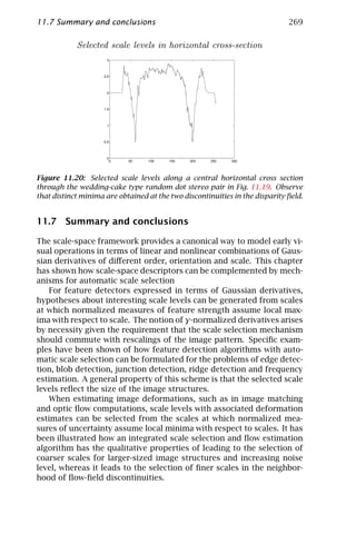
![270 11 Principles for Automatic Scale Selection
The material in this chapter is based on [3, chapter 13], [30], [35]
and [50]; see also [53] for a complementary work. Applications of these
scale selection principles to various problems in computer vision have
been presented in [44, 54, 55, 56, 57, 58, 59]. For related works see
[33, 36, 60, 61, 62, 63, 64, 65, 66, 67, 68, 69, 70].
11.8 References
[1] Koenderink, J. J., (1990). Solid Shape. Cambridge, Massachusetts: MIT
Press.
[2] Koenderink, J. J., Kaeppers, A., and van Doorn, A. J., (1992). Local Oper-
ations: The Embodiment of Geometry. In Artificial and Biological Vision
Systems, G. Orban and H.-H. Nagel, eds., pp. 1–23.
[3] Lindeberg, T., (1994). Scale-Space Theory in Computer Vision. The Kluwer
International Series in Engineering and Computer Science. Dordrecht,
Netherlands: Kluwer Academic Publishers.
[4] Babaud, J., Witkin, A. P., Baudin, M., and Duda, R. O., (1986). Uniqueness of
the Gaussian Kernel for Scale-Space Filtering. IEEE Trans. Pattern Analysis
and Machine Intell., 8(1):26–33.
[5] Florack, L. M. J., (1993). The Syntactical Structure of Scalar Images. , Dept.
Med. Phys. Physics, Univ. Utrecht, NL-3508 Utrecht, Netherlands.
[6] Florack, L. M. J., (1997). Image Structure. Series in Mathematical Imaging
and Vision. Dordrecht, Netherlands: Kluwer Academic Publishers.
[7] Florack, L. M. J., ter Haar Romeny, B. M., Koenderink, J. J., and
Viergever, M. A., (1992). Scale and the Differential Structure of Images.
Image and Vision Computing, 10(6):376–388.
[8] Florack, L. M. J., ter Haar Romeny, B. M., Koenderink, J. J., and
Viergever, M. A., (1993). Cartesian Differential Invariants in Scale-Space.
J. of Mathematical Imaging and Vision, 3(4):327–348.
[9] Hummel, R. A. and Moniot, R., (1989). Reconstructions from zero-
crossings in scale-space. IEEE Trans. Acoustics, Speech and Signal Pro-
cessing, 37(12):2111–2130.
[10] Koenderink, J. J., (1984). The structure of images. Biological Cybernetics,
50:363–370.
[11] Koenderink, J. J. and van Doorn, A. J., (1987). Representation of Local
Geometry in the Visual System. Biological Cybernetics, 55:367–375.
[12] Koenderink, J. J. and van Doorn, A. J., (1990). Receptive Field Families.
Biological Cybernetics, 63:291–298.
[13] Koenderink, J. J. and van Doorn, A. J., (1992). Generic neighborhood op-
erators. IEEE Trans. Pattern Analysis and Machine Intell., 14(6):597–605.
[14] Lindeberg, T., (1990). Scale-Space for Discrete Signals. IEEE Trans. Pattern
Analysis and Machine Intell., 12(3):234–254.
[15] Lindeberg, T., (1994). On the Axiomatic Foundations of Linear Scale-
Space: Combining Semi-Group Structure with Causality vs. Scale Invari-
ance. Technical Report ISRN KTH/NA/P--94/20--SE, Dept. of Numerical](https://image.slidesharecdn.com/computervision-handbookofcomputervisionandapplicationsvolume2-signalprocessingandpatternrecognition-120205081400-phpapp02/85/Computer-vision-handbook-of-computer-vision-and-applications-volume-2-signal-processing-and-pattern-recognition-295-320.jpg)
![11.8 References 271
Analysis and Computing Science, KTH, Stockholm, Sweden. Extended ver-
sion to appear in J. Sporring and M. Nielsen and L. Florack and P. Johansen
(eds.) Gaussian Scale-Space Theory: Proc. PhD School on Scale-Space The-
ory, Copenhagen, Denmark, Kluwer Academic Publishers, May 1996.
[16] Lindeberg, T., (1997). Linear spatio-temporal scale-space. In Scale-Space
Theory in Computer Vision: Proc. First Int. Conf. Scale-Space’97, B. M. ter
Haar Romeny, L. M. J. Florack, J. J. Koenderink, and M. A. Viergever, eds.,
Vol. 1252 of Lecture Notes in Computer Science, pp. 113–127. Utrecht, The
Netherlands: Springer Verlag, New York.
[17] Pauwels, E. J., Fiddelaers, P., Moons, T., and van Gool, L. J., (1995). An
extended class of scale-invariant and recursive scale-space filters. IEEE
Trans. Pattern Analysis and Machine Intell., 17(7):691–701.
[18] Sporring, J., Nielsen, M., Florack, L., and Johansen, P. (eds.), (1996). Gaus-
sian Scale-Space Theory: Proc. PhD School on Scale-Space Theory. Series
in Mathematical Imaging and Vision. Copenhagen, Denmark: Kluwer Aca-
demic Publishers.
[19] Yuille, A. L. and Poggio, T. A., (1986). Scaling Theorems for Zero-
Crossings. IEEE Trans. Pattern Analysis and Machine Intell., 8:15–25.
[20] Lindeberg, T., (1994). Scale-Space Theory: A Basic Tool for Analysing
Structures at Different Scales. Journal of Applied Statistics, 21(2):225–
270. Supplement Advances in Applied Statistics: Statistics and Images:
2.
[21] Lindeberg, T., (1996). Scale-space theory: A framework for handling im-
age structures at multiple scales. In Proc. CERN School of Computing, pp.
27–38. Egmond aan Zee, The Netherlands. Tech. Rep. CERN 96-08.
[22] Lindeberg, T. and ter Haar Romeny, B., (1994). Linear Scale-Space I:
Basic Theory. In Geometry-Driven Diffusion in Computer Vision, B. ter
Haar Romeny, ed., Series in Mathematical Imaging and Vision, pp. 1–41.
Dordrecht, Netherlands: Kluwer Academic Publishers.
[23] Lindeberg, T. and ter Haar Romeny, B., (1994). Linear Scale-Space II: Early
visual operations. In Geometry-Driven Diffusion in Computer Vision, B. ter
Haar Romeny, ed., Series in Mathematical Imaging and Vision, pp. 43–77.
Dordrecht, Netherlands: Kluwer Academic Publishers.
[24] Freeman, W. T. and Adelson, E. H., (1990). Steerable filters for early vision,
image analysis and wavelet decomposition. In Proc. 3rd Int. Conf. on
Computer Vision. Osaka, Japan: IEEE Computer Society Press.
[25] Perona, P., (1992). Steerable-Scalable Kernels for Edge Detection and Junc-
tion Analysis. In Proc. 2nd European Conf. on Computer Vision, pp. 3–18.
Santa Margherita Ligure, Italy.
[26] Bigün, J., Granlund, G. H., and Wiklund, J., (1991). Multidimensional ori-
entation estimation with applications to texture analysis and optical flow.
IEEE Trans. Pattern Analysis and Machine Intell., 13(8):775–790.
[27] Rao, A. R. and Schunk, B. G., (1991). Computing oriented texture fields.
CVGIP: Graphical Models and Image Processing, 53(2):157–185.
[28] Young, R. A., (1985). The Gaussian Derivative Theory of Spatial Vision:
Analysis of Cortical Cell Receptive Field Line-Weighting Profiles. Techni-](https://image.slidesharecdn.com/computervision-handbookofcomputervisionandapplicationsvolume2-signalprocessingandpatternrecognition-120205081400-phpapp02/85/Computer-vision-handbook-of-computer-vision-and-applications-volume-2-signal-processing-and-pattern-recognition-296-320.jpg)
![272 11 Principles for Automatic Scale Selection
cal Report GMR-4920, Computer Science Department, General Motors Re-
search Lab., Warren, Michigan.
[29] Young, R. A., (1987). The Gaussian derivative model for spatial vision: I.
Retinal mechanisms. Spatial Vision, 2:273–293.
[30] Lindeberg, T., (1996). Feature detection with automatic scale selection.
Technical Report ISRN KTH/NA/P--96/18--SE, Dept. of Numerical Analysis
and Computing Science, KTH, Stockholm, Sweden. Extended version in
Int. J. of Computer Vision, vol 30, number 2, 1998. (In press).
[31] Field, D. J., (1987). Relations between the statistics of natural images
and the response properties of cortical cells. J. of the Optical Society of
America, 4:2379–2394.
[32] Canny, J., (1986). A Computational Approach to Edge Detection. IEEE
Trans. Pattern Analysis and Machine Intell., 8(6):679–698.
[33] Korn, A. F., (1988). Toward a Symbolic Representation of Intensity
Changes in Images. IEEE Trans. Pattern Analysis and Machine Intell., 10
(5):610–625.
[34] Lindeberg, T., (1993). Discrete Derivative Approximations with Scale-
Space Properties: A Basis for Low-Level Feature Extraction. J. of Math-
ematical Imaging and Vision, 3(4):349–376.
[35] Lindeberg, T., (1996). Edge Detection and Ridge Detection with Automatic
Scale Selection. Technical Report ISRN KTH/NA/P--96/06--SE, Dept. of Nu-
merical Analysis and Computing Science, KTH, Stockholm, Sweden. Also
in Proc. IEEE Comp. Soc. Conf. on Computer Vision and Pattern Recogni-
tion, 1996. Extended version in Int. J. of Computer Vision, vol 30, number
2, 1998. (In press).
[36] Eberly, D., Gardner, R., Morse, B., Pizer, S., and Scharlach, C., (1994).
Ridges for Image Analysis. J. of Mathematical Imaging and Vision, 4(4):
353–373.
[37] Haralick, R. M., (1983). Ridges and valleys in digital images. Computer
Vision, Graphics, and Image Processing, 22:28–38.
[38] Koenderink, J. J. and van Doorn, A. J., (1994). Two-plus-one-dimensional
differential geometry. Pattern Recognition Letters, 15(5):439–444.
[39] Blostein, D. and Ahuja, N., (1989). Shape from texture: integrating texture
element extraction and surface estimation. IEEE Trans. Pattern Analysis
and Machine Intell., 11(12):1233–1251.
[40] Marr, D., (1982). Vision. W.H. Freeman, New York.
[41] Voorhees, H. and Poggio, T., (1987). Detecting Textons and Texture
Boundaries in Natural Images. In Proc. 1st Int. Conf. on Computer Vision.
London, England.
[42] Kitchen, L. and Rosenfeld, A., (1982). Gray-Level Corner Detection. Pattern
Recognition Letters, 1(2):95–102.
[43] Koenderink, J. J. and Richards, W., (1988). Two-Dimensional Curvature
Operators. J. of the Optical Society of America, 5:7:1136–1141.
[44] Lindeberg, T., (1997). On Automatic Selection of Temporal Scales in
Time-Casual Scale-Space. In Proc. AFPAC’97: Algebraic Frames for the
Perception-Action Cycle, G. Sommer and J. J. Koenderink, eds., Vol. 1315](https://image.slidesharecdn.com/computervision-handbookofcomputervisionandapplicationsvolume2-signalprocessingandpatternrecognition-120205081400-phpapp02/85/Computer-vision-handbook-of-computer-vision-and-applications-volume-2-signal-processing-and-pattern-recognition-297-320.jpg)
![11.8 References 273
of Lecture Notes in Computer Science, pp. 94–113. Kiel, Germany: Springer
Verlag, Berlin.
[45] Förstner, W. A. and Gülch, E., (1987). A Fast Operator for Detection and
Precise Location of Distinct Points, Corners and Centers of Circular Fea-
tures. In Proc. Intercommission Workshop of the Int. Soc. for Photogram-
metry and Remote Sensing. Interlaken, Switzerland.
[46] Lindeberg, T., (1994). Junction detection with automatic selection of de-
tection scales and localization scales. In Proc. 1st International Confer-
ence on Image Processing, Vol. I, pp. 924–928. Austin, Texas: IEEE Com-
puter Society Press.
[47] Bergen, J. R., Anandan, P., Hanna, K. J., and Hingorani, R., (1992). Hier-
archical Model-Based Motion Estimation. In Proc. 2nd European Conf. on
Computer Vision, G. Sandini, ed., Vol. 588 of Lecture Notes in Computer
Science, pp. 237–252. Santa Margherita Ligure, Italy: Springer-Verlag.
[48] Förstner, W. A., (1993). Image Matching. In Computer and Robot Vision,
R. M. Haralick and L. G. Shapiro, eds., Vol. II, pp. 289–378. Addison-Wesley.
[49] Lindeberg, T., (1995). Direct Estimation of Affine Deformations of Bright-
ness Patterns Using Visual Front-End Operators with Automatic Scale Se-
lection. In Proc. 5th International Conference on Computer Vision, pp.
134–141. Cambridge, MA.
[50] Lindeberg, T., (1996). A Scale Selection Principle for Estimating Image
Deformations. Technical Report ISRN KTH/NA/P--96/16--SE, Dept. of Nu-
merical Analysis and Computing Science, KTH, Stockholm, Sweden. Image
and Vision Computing (In press).
[51] Lukas, B. D. and Kanade, T., (1981). An iterative image registration tech-
nique with an application to stereo vision. In Image Understanding Work-
shop.
[52] Horn, B. K. P. and Schunck, B. G., (1981). Determining Optical Flow. J. of
Artificial Intelligence, 17:185–204.
[53] Lindeberg, T., (1993). Detecting salient blob-like image structures and
their scales with a scale-space primal sketch: A method for focus-of-
attention. Int. J. of Computer Vision, 11(3):283–318.
[54] Lindeberg, T. and Gårding, J., (1997). Shape-adapted smoothing in esti-
mation of 3-D depth cues from affine distortions of local 2-D structure.
Image and Vision Computing, 15:415–434.
[55] Gårding, J. and Lindeberg, T., (1996). Direct computation of shape cues
using scale-adapted spatial derivative operators. Int. J. of Computer Vi-
sion, 17(2):163–191.
[56] Lindeberg, T. and Li, M., (1997). Segmentation and classification of edges
using minimum description length approximation and complementary
junction cues. Computer Vision and Image Understanding, 67(1):88–98.
[57] Bretzner, L. and Lindeberg, T., (1998). Feature tracking with automatic
selection of spatial scales. Computer Vision and Image Understanding,
71(3):385–392. (To appear).](https://image.slidesharecdn.com/computervision-handbookofcomputervisionandapplicationsvolume2-signalprocessingandpatternrecognition-120205081400-phpapp02/85/Computer-vision-handbook-of-computer-vision-and-applications-volume-2-signal-processing-and-pattern-recognition-298-320.jpg)
![274 11 Principles for Automatic Scale Selection
[58] Almansa, A. and Lindeberg, T., (1996). Fingerprint enhancement by shape
adaptation of scale-space operators with automatic scale selection. in
preparation.
[59] Wiltschi, K., Pinz, A., and Lindeberg, T., (1997). Classification of Carbide
Distributions using Scale Selection and Directional Distributions. In Proc.
4th International Conference on Image Processing, Vol. II, pp. 122–125,
IEEE. Santa Barbara, California.
[60] Mallat, S. G. and Zhong, S., (1992). Characterization of Signals from Multi-
Scale Edges. IEEE Trans. Pattern Analysis and Machine Intell., 14(7):710–
723.
[61] Mallat, S. G. and Hwang, W. L., (1992). Singularity Detection and Process-
ing with Wavelets. IEEE Trans. Information Theory, 38(2):617–643.
[62] Zhang, W. and Bergholm, F., (1993). An Extension of Marr’s Signature
Based Edge Classification and Other Methods for Determination of Dif-
fuseness and Height of Edges, as Well as Line Width. In Proc. 4th Int.
Conf. on Computer Vision, H.-H. N. et. al., ed., pp. 183–191. Berlin, Ger-
many: IEEE Computer Society Press.
[63] Pizer, S. M., Burbeck, C. A., Coggins, J. M., Fritsch, D. S., and Morse, B. S.,
(1994). Object shape before boundary shape: Scale-space medial axis. J.
of Mathematical Imaging and Vision, 4:303–313.
[64] Koller, T. M., Gerig, G., Szèkely, G., and Dettwiler, D., (1995). Multiscale
Detection of Curvilinear Structures in 2-D and 3-D Image Data. In Proc. 5th
International Conference on Computer Vision, pp. 864–869. Cambridge,
MA.
[65] Jägersand, M., (1995). Saliency Maps and Attention Selection in Scale and
Spatial Coordinates: An Information Theoretic Approach. In Proc. 5th
International Conference on Computer Vision, pp. 195–202. Cambridge,
MA.
[66] Kanade, T. and Okutomi, M., (1994). A Stereo Matching Algorithm with an
Adaptive Window: Theory and Experiment. IEEE Trans. Pattern Analysis
and Machine Intell., 16(9):920–932.
[67] Battiti, R., Amaldi, E., and Koch, C., (1990). Computing Optical Flow Across
Multiple Scales: An Adaptive Coarse-to-Fine Strategy. Int. J. of Computer
Vision, 6(2):133–145.
[68] Niessen, W. and Maas, R., (1996). Optic Flow and Stereo. In Gaussian
Scale-Space Theory: Proc. PhD School on Scale-Space Theory, J. Sporring,
M. Nielsen, L. Florack, and P. Johansen, eds. Copenhagen, Denmark:
Kluwer Academic Publishers.
[69] Elder, J. H. and Zucker, S. W., (1996). Local scale control for edge detec-
tion and blur estimation. In Proc. 4th European Conference on Computer
Vision, Vol. 1064 of Lecture Notes in Computer Science. Cambridge, UK:
Springer Verlag, Berlin.
[70] Yacoob, Y. and Davis, L. S., (1997). Estimating Image Motion Using Tempo-
ral Multi-Scale Models of Flow and Acceleration. In Motion-Based Recog-
nition, M. Shah and R. Jain, eds. Kluwer Academic Publishers.](https://image.slidesharecdn.com/computervision-handbookofcomputervisionandapplicationsvolume2-signalprocessingandpatternrecognition-120205081400-phpapp02/85/Computer-vision-handbook-of-computer-vision-and-applications-volume-2-signal-processing-and-pattern-recognition-299-320.jpg)
![276 12 Texture Analysis
12.1 Importance of texture
12.1.1 Definition and background
Among other object properties such as color, shape, or motion, tex-
ture is one of the most prominent image attributes in both human and
automatic image analysis.
There are a number of different definitions for texture [1]. What all
definitions have in common is the fact that they describe texture as an
attribute of an image window. This attribute represents both
• spatially deterministic aspects of the gray levels (Fig. 12.1a);
• spatially stochastic aspects of the gray levels (Fig. 12.1b); and
• spatial aspects of color distribution.
In automatic image analysis, those attributes are represented by tex-
tural features, which are real numbers calculated from the image win-
dows with the help of functions such as those described below. The
number of potential textural features is large. Because some of them
are to a certain extent invariant with respect to change in illumination,
distortions, or scaling, they can also make an important contribution
to both object segmentation and object recognition tasks.
The human visual system can also distinguish between different
types of texture. From our daily experience, we know that we are capa-
ble of distinguishing between regular textures that differ in their ori-
entation, scale, phase, color, etc. For stochastic textures, differences in
the mean gray values or the variance will be noticed. Experiments on
the human visual perception of texture have already been performed
by Julesz [2]. A broad overview of this topic is given in Pratt [1].
Nevertheless, the way the human brain analyzes texture has not
yet been fully understood. Though there are cell complexes that de-
tect color, shape, or orientations, similar representations of textural
attributes in the brain have not yet been found. Some artificial textural
features may be based on biological models, but no biological repre-
sentation of the large variety of complex artificial textural features is
known. In that sense, texture analysis is a very complex problem for the
human visual system, which might partially be performed on a higher
level in the brain.
12.1.2 Texture analysis in machine vision
Texture analysis is also a demanding task for artificial machine vision
systems. The computation of textural features such as those described
in the following requires significantly more time and memory than the
extraction of simple geometric or color-based features. A rough esti-](https://image.slidesharecdn.com/computervision-handbookofcomputervisionandapplicationsvolume2-signalprocessingandpatternrecognition-120205081400-phpapp02/85/Computer-vision-handbook-of-computer-vision-and-applications-volume-2-signal-processing-and-pattern-recognition-301-320.jpg)
![12.1 Importance of texture 277
a b
Figure 12.1: a Determinstic texture: a brick wall; b stochastic texture: a tiled
floor.
mate is an average of 100 to 1000 operations per pixel for any textural
feature.
The demand for vast computing power can be either satisfied by
relying on special image processing hardware or by using clusters of
standard computer processing units (CPUs). A number of comparisons
between these hardware concepts suggests that for many practical ap-
plications of complex texture analysis the benefit of special hardware
is less than a factor of 2 in terms of speed [3] (see also Volume 3, Sec-
tion 3.2). At the same time, special hardware usually causes time delays
during the development process, and considerable costs when porting
solutions to a new (and quicker) hardware platform. For these reasons,
in the author’s opinion one can observe a clear shift towards standard
hardware solutions in industrial texture analysis applications. Never-
theless, this position is controversial (see also Volume 3, Chapters 2
and 3 and Chapter 11).
In any case, a large variety of technical applications benefit from
texture analysis:
• Surface inspection is essential for industrial quality control of wood,
fabrics, or metal surfaces;
• In object recognition, textural features can complement other object
attributes such as color or shape; and
• Finally, object segmentation profits from invariance properties of
textural features with respect to rotation, illumination, or scaling.
The literature reports a number of different methods for texture
analysis. In Section 12.2, some of the most prominent feature sets are](https://image.slidesharecdn.com/computervision-handbookofcomputervisionandapplicationsvolume2-signalprocessingandpatternrecognition-120205081400-phpapp02/85/Computer-vision-handbook-of-computer-vision-and-applications-volume-2-signal-processing-and-pattern-recognition-302-320.jpg)
![278 12 Texture Analysis
introduced. This section will give the reader an idea of the basic concept
of each feature set. Furthermore, it will allow the reader to implement
those feature sets. For further reading, especially on details of the the-
oretical background, links to the corresponding original publications
are given.
The list of textural feature sets given below is in no way complete,
but tries to give an overview of the variety of different models. The
author appreciates feedback on other important feature sets to be in-
cluded.
Section 12.3 compares the performance of the different textural fea-
ture sets. For this task, benchmark sets from different fields of texture
analysis are defined. Some of the sets are included on the attached
CD rom (.) The performance comparison covers the aspects of speed
and error rate in the recognition mode. Though this comparison is in
no way exhaustive, it might indicate how to proceed in order to find
adequate textural feature sets for a given problem.
Section 12.4 briefly shows that a quantitative evaluation of feature
performance can serve as a basis for automatic design of texture anal-
ysis systems. As a method of reducing both development costs and
time to market for image processing products, automatic design con-
cepts have recently attracted increasing attention.
12.2 Feature sets for texture analysis
There are numerous broader theoretical reviews on texture analysis
algorithms [4, 5]. Some papers compare the actual performance of fea-
ture sets, quite often on the basis of the Brodatz database (see [6] for
an electronic version) or the Vistex [7] image set. There are also web
sites containing benchmarks on some groups of textural features, such
as the Meastex benchmark [8].
In this chapter, we compare the performance of 318 textural fea-
tures from 18 feature sets. Because a benchmark can only be done
on a common data basis, we define 7 data sets as a basis for bench-
marking experiments. The available data sets can be used for further
comparisons.
Table 12.1 gives an overview of the different feature sets, which
are described in some more detail in this section. More details on the
implementation can be found in the given references. The intention of
the descriptions below is to provide the reader with a quick overview
of the methods and to describe the parameter configurations we have
used for our tests.](https://image.slidesharecdn.com/computervision-handbookofcomputervisionandapplicationsvolume2-signalprocessingandpatternrecognition-120205081400-phpapp02/85/Computer-vision-handbook-of-computer-vision-and-applications-volume-2-signal-processing-and-pattern-recognition-303-320.jpg)
![12.2 Feature sets for texture analysis 279
Table 12.1: Overview of feature sets for texture analysis, with number of
features per set and theoretical principle
No. Principle
Haralick 14 gray-level co-occurrence matrix
Unser 32 sum and difference histograms
Galloway 20 gray-level run lengths
Laine 21 wavelet packet signatures
Local 14 direct functions of gray values
Fractal (1) 10 fractal box dimension
Fractal (2) 47 fractal dimension from blankets
Laws 14 Laws’ convolution matrices
Fourier coeff. 33 energy in ring-shaped regions of Fourier space
Chen 16 geometric properties from binary image planes
Sun et al. 5 modified Haralick approach
Pikaz et al. 31 pyramid decomposition
Gabor 12 Gabor wavelets
Markov 7 Markov random fields
Dapeng 13 gray-level difference co-occurrence
Amadasun 5 neighboring difference histogram
Mao et al. 6 autoregressive models
Amelung 18 histogram and gradient features
Total: 318 No. of feature sets: 18
12.2.1 Haralick’s gray-level co-occurrence features
The feature set of Haralick et al. [10] is probably one of the most fa-
mous methods of texture analysis. It is based on the calculation of the
co-occurrence matrix, a second-order statistics of the gray levels in the
Har
image window. The co-occurrence matrix Pd,α (g, g ) counts the num-
ber of pixel pairs (m, n) and (m , n ) in an image that have intensity
values of g and g and that are separated by a pixel distance d in a
relative direction α.
In many cases, only eight neighbors and the corresponding four
directions α = 0°, 45°, 90° and 135° are taken into consideration. With
the definitions Lx = {1, 2, . . . , N } and Ly = {1, 2, . . . , M }, this leads to](https://image.slidesharecdn.com/computervision-handbookofcomputervisionandapplicationsvolume2-signalprocessingandpatternrecognition-120205081400-phpapp02/85/Computer-vision-handbook-of-computer-vision-and-applications-volume-2-signal-processing-and-pattern-recognition-304-320.jpg)
![12.2 Feature sets for texture analysis 281
Table 12.3: Features in Haralick’s co-occurrence-based method for texture
analysis.
Feature Definition
G G
2
Angular second momentum F Har =
ASM (p(g, g ))
g =1g =1
G−1 G G
Contrast F Har = g2 p(g , g )
Con
g =0 g =1g =1
|g −g =g |
G G
Correlation F Har = 1 (gg )p(g, g ) − µx µy
Cor σx σy
g =1g =1
G G
Sum of squares: variance F Har =
SSV (g − µ)2 p(g, g )
g =1g =1
G G
1
Inverse difference moment F Har =
IDM 1+(g −g )2
p(g, g )
g =1g =1
2G
Sum average F Har =
SAv g px +y (g)
g =2
2G
Sum variance1 F Har =
SVa (g − F Har )2 px +y (g)
SAv
g =2
2G
Sum entropy2 F Har = −
SEn px +y (g) log{px +y (g)}
g =2
G G
Entropy F Har = −
Ent p(g, g ) log{p(g, g )}
g =1g =1
G−1 G−1
Difference variance F Har =
DVa (px −y (g)(g − g px −y (g ))2 )
g =0 g =0
G−1
Difference entropy F Har = −
DEn px −y (g) log{px −y (g)}
g =0
Information measures of HXY −HXY 1
F Har =
correlation3 IC1 max{HX,HY }
F Har = (1 − exp[−2.0|HXY 2 − HXY |])1/2
IC2
Max. correlation coefficient4 F Har = (second largest eigenvalue of Q)1/2
MCC
1 In the original paper of Haralick, this feature depends on F Har instead of F Har , but
SEn SAv
we assume this to be a typographic error.
2 Forall Haralick features, expressions containing a log(0) term are simply sup-
pressed and do not contribute to the respective feature.
3 In the original paper of Haralick, there are no absolute values. We have added them
to avoid negative numbers in the argument of the square root function.
4 If the second largest eigenvalue is negative, the feature is set to 0. The calculation
of the eigenvalue has been performed with a routine from Press [9].](https://image.slidesharecdn.com/computervision-handbookofcomputervisionandapplicationsvolume2-signalprocessingandpatternrecognition-120205081400-phpapp02/85/Computer-vision-handbook-of-computer-vision-and-applications-volume-2-signal-processing-and-pattern-recognition-306-320.jpg)
![282 12 Texture Analysis
Har Har
Pd,90° (g, g ) and Pd,135° (g, g ) have equivalent definitions. In the pre-
ceding equations, the card operator denotes the number of elements in
a set.
For the actual evaluation, different methods of processing the co-
occurrence matrices are known. In our case, the four co-occurrence
matrices for the different directions and distance d = 1 are averaged:
Har 1
PΣ = P Har + P1,45° + P1,90° + P1,135°
Har Har Har
(12.2)
4 1,0°
A normalized co-occurrence matrix is calculated from
1 Har
p Har (g, g ) = PΣ (g, g ) (12.3)
Npixpair
with Npixpair as the total number of pixel pairs in the image
G G
Har
Npixpair = PΣ (g, g ) (12.4)
g =1g =1
In order to reduce the size of the co-occurrence matrices and to speed
up calculations, we have reduced the intensity resolution of the input
image down to 128 gray levels. The letter G represents the number of
distinct gray levels in the image after gray-level reduction. Additional
definitions are listed in Table 12.2.
Fourteen features are calculated from the normalized co-occurrence
matrix p Har (g, g ) (see Table 12.3).
12.2.2 Unser’s sum and difference histograms
In order to reduce the computation time necessary to calculate the co-
occurrence matrix, Unser has suggested a method to estimate its co-
efficients using a first-order statistic on the image window [11]. He
suggests sum and difference histograms on the gray levels.
Two image windows with centers at Gm,n and Gm ,n are displaced
by a distance d = (d1 , d2 )
Gm ,n = Gm+d1 ,n+d2 (12.5)
With the definition for the sum sm,n and the difference dm,n of the
respective gray levels
sm,n = Gm,n + Gm+d1 ,n+d2 and dm,n = Gm,n − Gm+d1 ,n+d2 (12.6)
the sum and difference histograms hs and hd are defined as follows:
hs (i; d1 , d2 ) = hs (i) = card{Gm,n |sm,n = i}
hd (j; d1 , d2 ) = hd (j) = card{Gm,n |dm,n = j } (12.7)](https://image.slidesharecdn.com/computervision-handbookofcomputervisionandapplicationsvolume2-signalprocessingandpatternrecognition-120205081400-phpapp02/85/Computer-vision-handbook-of-computer-vision-and-applications-volume-2-signal-processing-and-pattern-recognition-307-320.jpg)
![12.2 Feature sets for texture analysis 283
Table 12.4: Unser’s sum and difference histogram features.
Feature Definition
G−1
Mean F Uns =
Mea
ˆ
iP (i)
i=0
G−1
Angular Second Momentum F Uns =
ASM
ˆ
(P (i))2
i=0
G−1
Contrast F Uns =
Con
ˆ
(i − µ)2 P (i)
i=0
G−1
Entropy F Uns =
Ent
ˆ ˆ
− P (i)log P (i)
i=0
The number of total counts is
Ntot = card{G} = hs (i) = hd (j) (12.8)
i j
The histograms get normalized by
ˆ hs (i)
Ps (i) = , (i = 2, . . . 2G),
Ntot
(12.9)
ˆ hd (j)
Pd (j) = , (j = −G + 1, . . . G − 1)
Ntot
with G being the number of gray levels in the image. Typically, a re-
duced gray-level resolution (e. g., 32) is used.
ˆ ˆ
For both histograms Ps (i) and Pd (j), global features can be calcu-
lated according to Table 12.4. Doing this for all of the four possible
nearest displacements in the directions 0°, 45°, 90° and 135°, this leads
to a total of 32 Unser features.
12.2.3 Galloway’s run-length-based features
Galloway has proposed a run-length-based technique, which calculates
characteristic textural features from gray-level run lengths in different
image directions [12].
The basis of the calculation of the features is a run-length matrix
that is defined as
Gal
Pφ (g, r ) = (ag,r ) (12.10)
where ag,r is the number of occurrences of a connected pixel interval
of run length r in the direction φ with all pixel values of the interval
being equal to the gray-level value g.](https://image.slidesharecdn.com/computervision-handbookofcomputervisionandapplicationsvolume2-signalprocessingandpatternrecognition-120205081400-phpapp02/85/Computer-vision-handbook-of-computer-vision-and-applications-volume-2-signal-processing-and-pattern-recognition-308-320.jpg)
![284 12 Texture Analysis
Table 12.5: Definitions and features of Galloway’s run-length-based method
for texture analysis.
Abbreviations
Npix : number of pixels in image window
G: number of gray levels in image
R: maximal run length in image
G R
Gal
N= Pφ (g, r )
g =1 r =1
Feature Definition
G R Gal
Pφ (g,r )
1
Short run emphasis F Gal φ =
SRE, N l2
g =1 r =1
G R
1 Gal
Long run emphasis F Gal φ =
LRE, N l2 · Pφ (g, r )
g =1 r =1
2
G R
1 Gal
Gray-level distribution F Gal φ =
GLD, N Pφ (g, r )
g =1 r =1
2
R G
1 Gal
Run-length distribution F Gal φ =
RLD, N Pφ (g, r )
r =1 g =1
G R
1 Gal
Run percentage F Gal φ
RPe, = Npix r Pφ (g, r )
g =1 r =1
Usually, four run-length matrices for the directions φ = 0°, 45°, 90°,
and 135° are calculated. In order to get sufficiently high run-length
values, a reduction of the gray values of an image is performed, in our
case down to 16 values.
Table 12.5 shows the features derived from the four run-length ma-
trices. Because they are calculated for each of the four run-length ma-
trices, a total of 20 features is derived.
12.2.4 Chen’s geometric features from binary image sequences
Chen [13] decomposes a gray-level image into a sequence of binary
images and calculates a total of 16 features from geometric properties
of the resulting blob regions.
From the original image, a series of binary images Gbin,t is con-
structed by help of thresholds t ∈ 1, . . . G − 1 as follows:
bin,t 1 for Gm,n ≥ t
Gm,n = (12.11)
0 else
The features below are derived for each connected region I in the image,
with a 4-neighborhood relation as the basis of connectivity. With the](https://image.slidesharecdn.com/computervision-handbookofcomputervisionandapplicationsvolume2-signalprocessingandpatternrecognition-120205081400-phpapp02/85/Computer-vision-handbook-of-computer-vision-and-applications-volume-2-signal-processing-and-pattern-recognition-309-320.jpg)
![12.2 Feature sets for texture analysis 285
Table 12.6: Definitions and features of Chen’s binarization-based method for
texture analysis.
Abbreviations
Number of NOC0 (t): Number of connected black areas in bi-
connected areas nary image generated with threshold t.
NOC1 (t): Number of connected white areas in bi-
nary image generated with threshold t.
[NOPb (t,I)IRGLb (t,I)]
I ∈Gbin,t
Average irregularity IRGLb (t) = ; b ∈ {0, 1}
NOPb (t,I)
I ∈Gbin,t
Feature Definition
For each g(t) ∈ {IRGL0 (t), IRGL1 (t), NOC0 (t), NOC1 (t)} calculate
Maximum F Che = max1≤t ≤G−1 g(t)
Max
G−1
1
Average F Che =
Ave g(t)
G − 1 t =1
G−1 G−1
Mean F Che =
Mea tg(t) g(t)
t =1 t =1
G−1
1
Standard deviation F Che =
StD G−1
(t − F Che )2 g(t)
Mea
t =1
g(t)
t =1
definitions
x= xi |I |, y= yi |I | (12.12)
i∈I i ∈I
and |I | as the number of pixels in the area I, a center of gravity (x, y) is
calculated for each connected region I. The index i runs over all pixels
in a connected area I. For all connected areas I in ftbin , a measure of
irregularity is defined as
√
1 + π max i∈I (xi − x)2 + (yi − y)2
IRGLb (t, I) = −1 (12.13)
|I |
The parameter b denotes connected black areas b = 0 and white areas
for b = 1. The forementioned definitions serve, together with further
definitions of the parameters “number of connected areas” and “aver-
age irregularity,” as a basis of textural features derived from the se-
quence of binary images. Those features are listed in Table 12.6. In](https://image.slidesharecdn.com/computervision-handbookofcomputervisionandapplicationsvolume2-signalprocessingandpatternrecognition-120205081400-phpapp02/85/Computer-vision-handbook-of-computer-vision-and-applications-volume-2-signal-processing-and-pattern-recognition-310-320.jpg)
![286 12 Texture Analysis
our experiments, binary images are calculated with the 15 thresholds
t = 16, 32, 48, . . . , 240.
12.2.5 Laine’s textural energy from Daubechies wavelets
Laine uses a wavelet decomposition with Daubechies wavelets and takes
the energies in the different filter bands as features [14]. Details on
implementation including a 2-D implementation and the Daubechies
coefficients DAUB4 used here can be found in [9, Chapter 13.10].
Being interested in the application of wavelets it is sufficient to know
that, similar to a Fourier transformation, a wavelet transform repre-
sents a transformation to different orthogonal basis functions. While
for the Fourier Transform these basic functions are sine and cosine
functions, so called wavelets are used for the wavelet transform.
For the wavelet transform of a 1-D signal the transformation can
be expressed by use of a transformation matrix acting on the column
vector of the signal.
For the following discussion we concentrate on the transformation
coefficients of the DAUB4 wavelet transform used here, which is char-
acterized by the four coefficients c0 , . . . , c3 . The numerical values of the
DAUB4 coefficients are
c0 = 0.4829629131445341, c1 = 0.8365163037378079
(12.14)
c2 = 0.2241438680420134, c3 = −0.1294095225512604
In the case of a DAUB4 wavelet transform the transformation matrix
for a onedimensional signal with 8 components is
c0 c1 c2 c3 0 0 0 0
c3 −c 2 c1 −c 0 0 0 0 0
0 0 c0 c1 c2 c3 0 0
0 0 c3 −c 2 c1 −c0 0 0
W = (12.15)
0 0 0 0 c0 c1 c2 c3
0 0 0 0 c3 −c2 c1 −c0
c2 c3 0 0 0 0 c0 c1
c1 −c 0 0 0 0 0 c3 −c2
This transformation matrix can be interpreted as two different rota-
tions in the space of basic functions, which are interwoven. One rota-
tion operates on the even rows the other one on the odd rows. From
a practical point of view the filter coefficients in the odd rows can be
seen as a blurring filter while the coefficients in even rows perform a
sharpening.
After applying the transformation matrix once a permutation of the
resulting vector entries has to take place in order to “separate” the](https://image.slidesharecdn.com/computervision-handbookofcomputervisionandapplicationsvolume2-signalprocessingandpatternrecognition-120205081400-phpapp02/85/Computer-vision-handbook-of-computer-vision-and-applications-volume-2-signal-processing-and-pattern-recognition-311-320.jpg)
![12.2 Feature sets for texture analysis 287
Figure 12.2: Schematic figure of a wavelet transformation: An image is split
into four subimages of equal size.
two filter outputs from each other. As each rotation uses only half
the number of rows a rescaling of a factor of two takes place but two
outputs (in the vector below with 4 components each) are generated.
x1 s1 s1
x d s
2 1 2
x3 s2 s3
x
4 transformation d2 permutation s4
→ → (12.16)
x5 s3 d1
x d3 d2
6
x7 s4 d3
x8 d4 d4
In order to apply a wavelet transform to a 2-D image one has to trans-
form and reorder the rows and the columns of the image sequentially.
As in Fourier transforms the order of operation is not important. Each
transformation step generates four different subimages from one origi-
nal image (Fig. 12.2). The letters, for example, in the top right subimage
indicate the first transformation (e. g., on the rows) has been a sharp-
ening while the second one (on the columns) was a blurring.
While many wavelet transforms do a multiresolution analysis by
successively transforming only the top left subimage of each decom-
position step, Laine has decided to do the decomposition for all four
subimages successively.
For extracting textural features F Lai an energy value is calculated
for each subimage in a decomposition sequence by summing over the
squares of all pixel values in the subimage. With three resolution steps
in the wavelet decomposition 21 features can be calculated. One coeffi-
cient stems from the original image, four from the first decomposition
level, and further 16 from the second level.
12.2.6 Local textural features
Local texture features are calculated directly from the original image
window [15]. The feature set contains statistical features and gradient
features. In the case of the first feature (gray level of central pixel),](https://image.slidesharecdn.com/computervision-handbookofcomputervisionandapplicationsvolume2-signalprocessingandpatternrecognition-120205081400-phpapp02/85/Computer-vision-handbook-of-computer-vision-and-applications-volume-2-signal-processing-and-pattern-recognition-312-320.jpg)
![12.2 Feature sets for texture analysis 289
Table 12.8: Definitions of Kirsch matrices
5 5 5 5 5 −3 5 −3 −3
K 0 = −3 0 −3 K 1 = 5 0 −3 K 2 = 5 0 −3
−3 −3 −3 −3 −3 −3 5 −3 −3
−3 −3 −3 −3 −3 −3 −3 −3 −3
K3 = 5 0 −3 K 4 = −3 0 −3 K 5 = −3 0 5
5 5 −3 5 5 5 −3 5 5
−3 −3 5 −3 5 5
K 6 = −3 0 5 K 7 = −3 0 5
−3 −3 5 −3 −3 −3
Table 12.9: Definitions of Sobel operators
−1 −2 −1 −1 0 1
Sx = 0 0 0 S y = −2 0 2
1 2 1 −1 0 1
Local features of the input image are shown in Table 12.7. For an image
with G gray levels, median(G) is defined as
MN
median(G) = min{card{(m , n )|Gm ,n ≤ g } ≥ } (12.19)
g 2
The Kirsch matrices used for feature F Loc are shown in Table 12.8,
Kir
and the Sobel operators (essential for calculating feature F Loc ) are shown
Sob
in Table 12.9. The Sobel operator is discussed in detail in Section 10.3.4.
12.2.7 Fractal features
A number of different fractal features are in use. In Roß et al. [16],
fractal box dimensions are calculated on a set of binary images. These
images are generated from the original image with the help of thresh-
olds calculated from the maximal gradient value in the image.
From the original image G, a gradient image G is generated with
the help of a Sobel operator (see Table 12.9):
Gx Sx G
D= = (12.20)
Gy Sy G](https://image.slidesharecdn.com/computervision-handbookofcomputervisionandapplicationsvolume2-signalprocessingandpatternrecognition-120205081400-phpapp02/85/Computer-vision-handbook-of-computer-vision-and-applications-volume-2-signal-processing-and-pattern-recognition-314-320.jpg)
![290 12 Texture Analysis
An absolute value1 is calculated from the gradient image by
|D| = Gx · Gx + Gy · Gy (12.21)
Binarization is accomplished with a threshold t such that
1 if Dm,n > t
Gbin,t =
m,n (12.22)
0 else
A fractal box dimension is calculated by covering the binary image
with a lattice of grid size r and calculating the number of squares
Ng (Gbin,t , r ) containing pixels with value 1. From that, a fractal di-
mension D is calculated by means of linear regression2 from a double-
logarithmic plot of the equation
1
Ng (Gbin,t , r ) = (12.23)
rD
The authors of the original paper have spent some effort in adapting the
levels t for binarization to their data sample. Because our benchmark
tends to follow a more general approach, we have chosen the 10 values
ti = 25i, i ∈ 1, 2, . . . 10. The 10 resulting feature values are taken as
the feature set “Fractal (1).”
Another fractal feature set named “Fractal (2)” is defined in Peleg
et al. [17]. Peleg’s basic idea was to determine a fractal surface area by
covering the surface with “blankets.”
When covering a surface with a blanket of thickness 2 , the area of
the surface is calculated from dividing the blanket volume by 2 . The
covering blanket has an upper surface u and a lower surface b . With
the image gray levels Gm,n and initial conditions
u0 (m, n) = b0 (m, n) = Gm,n (12.24)
a sequence of blanket surfaces for different thicknesses is defined as
follows:
u (m, n) = max u −1 (m, n) + 1, max u −1 (m ,n )
|(m,n)−(m ,n )|≤1
b (m, n) = min b −1 (m, n) − 1, min b −1 (m ,n )
|(m,n)−(m ,n )|≤1
1 In our implementation, the argument of the square root is clipped to 255, and the
result of the square root is converted to an integer value.
2 In the regression all data points with N = 0 are suppressed; on a 64 × 64 pixel
g
image, Ng is calculated for grid sizes r = 2i , i ∈ {1, 2, . . . , 5}. For the implementation
of the linear regression, see [9].](https://image.slidesharecdn.com/computervision-handbookofcomputervisionandapplicationsvolume2-signalprocessingandpatternrecognition-120205081400-phpapp02/85/Computer-vision-handbook-of-computer-vision-and-applications-volume-2-signal-processing-and-pattern-recognition-315-320.jpg)
![12.2 Feature sets for texture analysis 291
For calculation of the blanket position in step , this recursive defini-
tion uses the gray values of the four neighbors in step − 1. With the
definitions
v = (u (m, n) − b (m, n)) (12.25)
m,n
for the volume v of the blanket and
(v − v −1 )
A( ) = (12.26)
2
for the surface area A( ) corresponding to a blanket radius , a fractal
dimension D is defined by
2− D
A( ) = F (12.27)
Slopes S are calculated from best fit lines through the three points
(log( − 1), log(A( − 1))),
(log( ), log(A( ))), (12.28)
(log( + 1), log(A( + 1)))
In our experiments, we use the slopes S( ) as textural features. From
49 area values A( ), = 1, . . . 49, 47 slopes S( ) can be extracted.
12.2.8 Laws filter masks for textural energy
Laws has suggested a set convolution masks for feature extraction [18].
There are five 1-D filter masks with the labels “level,” “edge,” “spot,”
“wave,” and “ripple” (Table 12.10). From them, 25 2-D filter masks can
be constructed, for example,
1 − 1 −2 0 2 1
4 − 4 −8 0 8 4
F le = l5 e 5 = 6 [−1, −2, 0, 2, 1] = −6 −12 0 12 6
T
(12.29)
4 − 4 −8 0 8 4
1 − 1 −2 0 2 1
The 14 Laws features are calculated from
gxy + gyx
F Law =
xy (12.30)
gll
where
gxy = |(x 5 y T ) ∗ G|, with x 5 , y 5 ∈ {l5 , e 5 , s 5 , w 5 , r 5 }
5 (12.31)
m n
Ten features are calculated from nondiagonal elements (x = y), while
another four stem from diagonal elements, and the fifth diagonal ele-
ment gll is used for normalization.](https://image.slidesharecdn.com/computervision-handbookofcomputervisionandapplicationsvolume2-signalprocessingandpatternrecognition-120205081400-phpapp02/85/Computer-vision-handbook-of-computer-vision-and-applications-volume-2-signal-processing-and-pattern-recognition-316-320.jpg)
![292 12 Texture Analysis
Table 12.10: Definitions of 1-D Laws matrices
Laws matrices
1 −1 −1 −1 1
4 −2 0 2 −4
l5 = 6
e5 = 0
s5 = 2
w5 = 0
r5 = 6
4 2 0 −2 −4
1 1 −1 1 1
12.2.9 Fourier features
In [16], energy values calculated from different regions in the power
spectrum of the images Fourier transform are taken as textural fea-
tures. A total of thirty-three Fourier coefficients are extracted for the
description of textures.
ˆ
The discrete Fourier transform G of a two-dimensional real image
G is defined as
M −1 N −1
ˆ 1 2π imu 2π inv
Gu,v = Gm,n exp − exp − (12.32)
MN m=0 n=0 M N
ˆ
The resulting power spectrum |G| is symmetrical (Section 3.3.3), there-
fore only the area {[u, v]|u ∈ {−M/2 + 1, . . . , M/2} ∧ v ∈ {0, . . . , N/2}
will be the basis of the calculations below.
If the image is quadratic, that is, M = N, radial features can be
defined as
cr1 ,r2 = ˆ
|Gu,v |2 (12.33)
2 2
r1 ≤u2 +v 2 ≤r2
The seven radial features F Fou . . . F Fou are calculated from
ra0 ra6
iN
F Fou = cri ,ri+1 ,
rai i ∈ 0, . . . 6, ri = (12.34)
72
An eighth radial feature F Fou is defined as the sum over the coefficients
ra7
in the “corners” of the Fourier domain, not included within the largest
circle. Summing over the coefficients in the respective circle segments
leads to energy values aθ1 ,θ2
aθ1 ,θ2 = ˆ
|Gu,v |2 (12.35)
v
θ1 ≤tan−1 u ≤θ2
They are the basis of the 10 directional features F Fou . . . F Fou defined by
di0 di9
iπ
F Fou = aθi ,θi+1 ,
dii θi = (i = 0, . . . 9) (12.36)
10](https://image.slidesharecdn.com/computervision-handbookofcomputervisionandapplicationsvolume2-signalprocessingandpatternrecognition-120205081400-phpapp02/85/Computer-vision-handbook-of-computer-vision-and-applications-volume-2-signal-processing-and-pattern-recognition-317-320.jpg)
![12.2 Feature sets for texture analysis 293
Finally, 10 horizontal and 5 vertical features are defined as
(i−1) 10 M +(− M +1)
1
2
N
2
F Fou
hoi = ˆ
|Gu,v |2 , i ∈ {0, . . . , 9} (12.37)
u=i 10 M +(− M +1) v =0
1
2
and
M
2 (i+1) 1
5
N
2
F Fou
vei = ˆ
|Gu,v |2 , i ∈ {0, . . . , 4} (12.38)
u=− M
2 +1 v =i 1 N
5 2
12.2.10 A modified gray-level co-occurrence approach
Sun and Wee [19] define five features from a modified Haralick ap-
proach. They calculated statistics in an 8-neighborhood and are there-
fore less dependent on image rotations.
The matrix PN (g, s, a, d) lists the number of pixels s in a neighbor-
hood N of an image point Gm,n , for which the gray-level difference
|Gm,n − Gm ,n | is lower or equal to a given threshold d. The neigh-
borhood is defined by a distance threshold ρ
Sun
PN,a,d (g, s) = card{(m, n)|Gm,n = g ∧
∧ card[(m , n )|ρ((m, n), (m , n )) ≤ a (12.39)
∧ |Gm,n − Gm ,n | ≤ d] = s }
In our implementation, the parameter values a = 0 and d = 1 are used.
Sun
From the matrix PN,a,d (g, s), five features are defined, which are shown
in Table 12.11.
12.2.11 Texture analysis from pyramid decomposition
Pikaz and Averbuch [20] calculate textural features from a sequence
of graphs {Ns (t)}, where Ns (t) denotes the number of 4-connected
structures of at least size s, and t denotes a threshold used to binarize
the image. They suggest an optimized implementation that computes
the sequence of graphs in almost linear time complexity in terms of
number of pixels in the image.
In this paper, we follow the suggestion of the Pikaz and Averbuch
to use {N2 (t)} to characterize a texture. As thresholds t(i) we choose
G−1
t(i) = i , i ∈ {0, 1, . . . , Nt − 2} (12.40)
Nt − 1
with G as the number of gray levels, and Nt the number of thresholds
to be determined. In our implementation, Nt is defined as 32, which
leads to a total of 31 features.](https://image.slidesharecdn.com/computervision-handbookofcomputervisionandapplicationsvolume2-signalprocessingandpatternrecognition-120205081400-phpapp02/85/Computer-vision-handbook-of-computer-vision-and-applications-volume-2-signal-processing-and-pattern-recognition-318-320.jpg)
![294 12 Texture Analysis
Table 12.11: Features from the modified Haralick approach by Sun and Wee
Abbreviations
G 8
Sun
N= PN,1,d (g, s)
g =1 s =0
Feature Definition
G 8 Sun
PN,1,d (g,s)
1
Small number emphasis F Sun =
SNE N s2
g =1 s =0
G 8
1
Large number emphasis F Sun =
LNE N s 2 · PN,1,d (g, s)
Sun
g =1 s =0
2
8 G
1
Number distribution F Sun =
NDi N
Sun
PN,1,d (g, s)
s =0 g =1
G 8
1
Angular second moment F Sun
ASM = N2
PN,1,d (g, s)2
Sun
g =1 s =0
G 8 P Sun (g,s)
−1
Entropy F Sun = PN,1,d (g, s) · ld( N,1,d
Sun
)
Ent ld( 81G ) N
· g =1 s =0
12.2.12 Gabor wavelets
Fogel and Sagi [21] and many others suggest the use of so-called Gabor
wavelets or Gabor filters for feature extraction. Gabor wavelets are de-
fined in Section 4.2.2. They can be used to extract a certain wavelength
and orientation from an image with a specified bandwidth. Because the
Gabor filter is a quadrature filter (Section 4.2), the “energy” of the signal
in the filter band can be determined by computing the square magni-
tude of the complex filter response. Here values for the wavelength λ
and the orientation θ are λ ∈ {2, 4, 8} and θ ∈ {0°, 45°, 90°, 135°}, which
leads to a total of 12 features.
12.2.13 Markov random field approach
In Kashyap et al. [22], a Markov random field approach is chosen to
extract seven different textural features. Markov random fields model
a texture by expressing all gray values of an image as a function of the
gray values in a neighborhood η of each pixel. Each pixel Gm ,n in this
neighborhood is characterized by its distance d = (d1 , d2 ) from the
central pixel Gm,n :
Gm ,n = Gm+d1 ,n+d2 (12.41)
For each image, one set of global model parameters {θd } is deter-
mined, which is characteristic of a special type of texture. This global](https://image.slidesharecdn.com/computervision-handbookofcomputervisionandapplicationsvolume2-signalprocessingandpatternrecognition-120205081400-phpapp02/85/Computer-vision-handbook-of-computer-vision-and-applications-volume-2-signal-processing-and-pattern-recognition-319-320.jpg)
![12.2 Feature sets for texture analysis 295
set of parameters model the neighborhoods of all pixels in an image.
As the fit will not be perfect, there is a remaining error
Gm,n = θd Gm ,n + m,n (12.42)
all Gm ,n ∈η
Figure 2.5b in Chapter 2 shows the neighboring pixels of a central pixel
x. They are ordered with respect to their distance. In our current im-
plementations, all neighbors 1, 2 and 3 are included in the model. How-
ever, one single model parameter represents a pair of point-symmetric
neighbors at a time, which are averaged. In our case, 12 neighboring
pixels help to fit six model parameters. The seventh parameter is the
standard deviation that describes the error in the least squares fit. The
fit is performed with a routine from Press [9].
12.2.14 Co-occurrence with average neighborhood
Dapeng and Zhongrong [23] construct a modified co-occurrence matrix
P Dap (g, d). It represents the co-occurrence between gray levels g in
the central pixel and a gray-level difference d. The gray-level difference
d is the difference between the central gray level g and the average gray
level of the eight neighboring pixels.
From this modified co-occurrence matrix, Dapeng extracts the 13
features shown in Table 12.12.
12.2.15 Co-occurrence histogram
Amadasun and King [24] use an approach similar to that of Dapeng, but
do not construct a 2-D co-occurrence matrix. Instead, they average the
differences for each gray-level value of the central pixel and construct
features from this histogram distribution
Ama
PT (i) = |Gm,n − Am,n | (12.43)
m n
Gm,n =i
where Am,n is the average of the gray levels of the eight neighboring
Ama
pixels of pixel (m, n). From the histogram PT (i) and the conven-
Ama
tional gray-tone histogram PH (i), Amadasun calculates the textural
features presented in Table 12.13.
12.2.16 Autoregressive models
Mao and Jain [25] use multiresolution simultaneous autoregressive mod-
els for texture classification. The basic idea of a simultaneous autore-
gressive (SAR) model is to express a gray level of a pixel as a function of
the gray levels in its neighborhood. The related model parameters for](https://image.slidesharecdn.com/computervision-handbookofcomputervisionandapplicationsvolume2-signalprocessingandpatternrecognition-120205081400-phpapp02/85/Computer-vision-handbook-of-computer-vision-and-applications-volume-2-signal-processing-and-pattern-recognition-320-320.jpg)
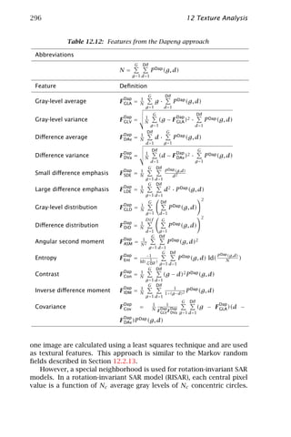
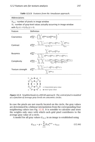
![298 12 Texture Analysis
Table 12.14: Features from the Amelung approach
Abbreviations
G
Number of pixels in image window: Npix = g =1 PH (g)
Feature Definition
Gw
1
Average F Ame =
Ave Npix PH (g) · g
g =1
Gw
1
Variance F Ame =
Var Npix PH (g) · (g − F Ame )2
Ave
g =1
Gw
1
3rd moment F Ame =
3Mo Npix PH (g) · (g − F Ame )3
Ave
g =1
Gw
1
4th moment F Ame =
4Mo Npix PH (g) · (g − F Ame )4
Ave
g =1
Gw
1
Angular second moment F Ame =
ASM 2
Npix
PH (g)2
g =1
Gw
−1 PH (g)
Entropy F Ame =
End 1 PH (g) · log( Npix )
log( G )
g =1
to determine the parameters θ1 , . . . , θNc , µ, σ from the image, with σ
being the standard deviation of and Nc being the number of circles
used per pixel. In our implementation, we have used four circles, which
leads to a total of six features.
A multiresolution SAR model calculates a sequence of image res-
olutions, for example, by means of a Gaussian pyramid, and deter-
mines model parameters for each image resolution. The collection of
all model parameters is used as a feature vector.
12.2.17 Statistical features
Amelung [26] has constructed a system called AST to evaluate a num-
ber of different statistical features from seven feature sets. The rest
of his features are already part of the foregoing discussion, therefore
only features extracted from gray level and gradient histograms are
combined in the features set discussed here.
Amelung’s features are shown in Table 12.14. For the histogram
PH (g) i the formulas of Table 12.14, three different histograms (gray
level histogram, histogram of absolute value and of direction of gradi-
ent) are used. A Sobel filter generates the gradient image.](https://image.slidesharecdn.com/computervision-handbookofcomputervisionandapplicationsvolume2-signalprocessingandpatternrecognition-120205081400-phpapp02/85/Computer-vision-handbook-of-computer-vision-and-applications-volume-2-signal-processing-and-pattern-recognition-323-320.jpg)
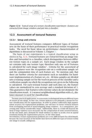
![300 12 Texture Analysis
Table 12.15: Data sets for benchmarking
Data sets
Brodatz Tumor Tilda Print Slab Vistex Hon
Abbreviation BRO 64 TUM 64 TIL 64 PRI 64 SLA 64 VIS 64 HON 64
Classes 13 2 6 26 11 15 6
Patterns per class
Training 64 72 1600 16 12 32 24
Testing 64 72 1600 8 12 32 24
Verification 128 71 1600 16 12 64 24
Window size 64 × 64 368 × 280 64 × 64 64 × 64 64 × 64 64 × 64 64 × 64
Bits per pixel 8 8 8 8 8 8 8
The calculation time is defined as time for calculating the floating
point vector of textural features from a 64 × 64 pixel image window.
The actual implementation was done on a Pentium 200 MHz PC with-
out MMX under Linux, Kernel Version 2.0.22 using the GNU g++ com-
piler, version 2.7.2.1. The calculation time was measured by averaging
over a data set with Brodatz images containing 65 image windows. A
comparison with other platforms can be performed on the basis of CPU
benchmarks. A simple linpack benchmark that can be performed per
internet using a java applet [27] has given a performance of 11.4 MFlops
for our computer.
12.3.2 Data sets for benchmarking
An overview of the underlying data sets is given in Table 12.15. The
number of classes in each data set is given as well as the patterns avail-
able per class. Note that all the data set have been divided into three
subsets each for training, testing, and verification. All the recognition
results given below were determined on the verification samples.
In order to allow the reader to benchmark his own textural feature
sets with the features given in this paper, we have included most of the
data sets in /images/12 on the CD-ROM. A general description of the
data sets is given in /images/12/readme.txt.
The testing sets are not used for any experiments in this paper, but
are included to serve as intermediate performance check when auto-
matically determining optimal feature subsets. While this will be one
focus of our future work, we have decided immediately to keep one
division of our data sets fixed. This will allow us to directly compare
the performance of the feature sets from the literature given in this pa-](https://image.slidesharecdn.com/computervision-handbookofcomputervisionandapplicationsvolume2-signalprocessingandpatternrecognition-120205081400-phpapp02/85/Computer-vision-handbook-of-computer-vision-and-applications-volume-2-signal-processing-and-pattern-recognition-325-320.jpg)
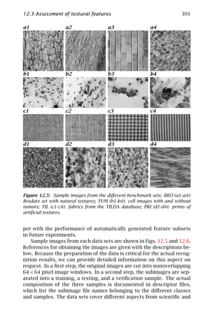
![302 12 Texture Analysis
e1 e2 e3 e4
f1 f2 f3 f4
g1 g2 g3 g4
Figure 12.6: Sample images from the different benchmark sets (II): SLA (e1-
e4): slabs of different type; VIS (f1-f4): natural images from the Vistex database;
HON (g1-g4): metal surfaces.
applied texture analysis. Some of them are established as benchmark
samples, others are quite new, but are both large and relevant.
The Brodatz sample (/images/12/bro) is a widespread benchmark sample
for the comparison of textural features. It consists of a collection of natural
textures. Our experiments are based on the electronic version from Weber [6],
which consists of 13 different classes.
In the tumor data sample (/images/12/tum), cell images from human spu-
tum are used for visual cancer diagnosis.This data set is the only one where
the textural features are calculated on the complete image without extracting
subimages. The reason for this is that each image contains regions of both
diseased and healthy cells, and the exact assignment is not known. For those
feature extraction methods which require quadratic input, the tumor images
have been stretched to a quadratic size of 256 × 256 pixel by means of bilin-
ear interpolation. Because the number of samples for the two classes was not
equal in this data set, the number of patterns per class given in Table 12.15 is
the minimum number for both classes.](https://image.slidesharecdn.com/computervision-handbookofcomputervisionandapplicationsvolume2-signalprocessingandpatternrecognition-120205081400-phpapp02/85/Computer-vision-handbook-of-computer-vision-and-applications-volume-2-signal-processing-and-pattern-recognition-327-320.jpg)
![12.3 Assessment of textural features 303
Recognition rates in %
Size of training and verification set
Figure 12.7: Recognition rates as a function of data set size for different data
sets. The error bars resemble the standard deviation calculated with randomly
chosen data sets.
Images of different fabrics are collected in the TILDA sample (see Schulz-
Mirbach [28]) and /images/12/til). The data have been collected within the
German research program “Automatische Sichtprüfung” (automatic visual in-
spection) of the “Deutsche Forschungsgemeinschaft” (DFG).
The print sample (/images/12/pri) consists of a collection of 26 different
textures from paper prints with imitations of natural wooden surfaces. Such
papers are used for coating chipboards, for example, for use in kitchens.
The slab sample (/images/12/sla) gives a collection of 11 different sur-
face types of slabs.
The Vistex benchmark sample ((/images/12/vis), see also [7]) contains a
collection of 15 different types of natural textures.
The Hon sample (/images/12/hon) contains images of metal surfaces. It
also stems from the research program “Automatische Sichtprüfung” and is
described in [29].
12.3.3 Experiments and results
We first wanted to determine the sensitivity of the recognition rates
with respect to the actual composition of the data set. For this reason,
we have calculated standard deviations of the recognition rates for dif-
ferent data set sizes n using the Galloway feature set. The size n is the
total number of image samples in the training set; the verification set
is of the same size.
The results are shown in Fig. 12.7. The error bars given resemble the
standard deviation σ , which was calculated on the basis of recognition
results from 120 randomly chosen data subset selections. As expected,
the recognition rates increase with growing training set sizes, while the
standard deviation decreases. For reliable results, a sample set size of
at least a few hundred images is a prerequisite. Table 12.16 gives the
details of the benchmarking experiments with the different textural fea-
ture sets on the seven data sets. The table lists the recognition results
and the feature extraction time on a 64 × 64 pixel image windows.](https://image.slidesharecdn.com/computervision-handbookofcomputervisionandapplicationsvolume2-signalprocessingandpatternrecognition-120205081400-phpapp02/85/Computer-vision-handbook-of-computer-vision-and-applications-volume-2-signal-processing-and-pattern-recognition-328-320.jpg)
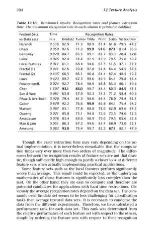
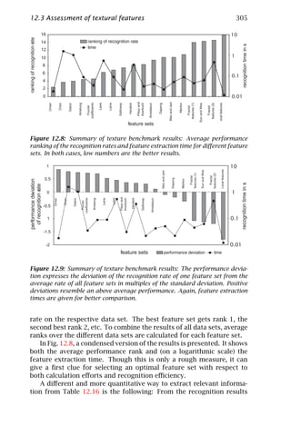
![306 12 Texture Analysis
of all feature sets for one data set, a mean value and a standard devi-
ation of the performance are calculated. From that, the difference of
each recognition result from the mean is expressed as a multiple of
the standard deviation for that data sample, which gives a quantitative
ranking of the performance of the different feature sets on one data
sample. We call this measure “performance deviation.” Summing the
performance deviation over all different data sets, one gets a character-
istic that is more quantitative than the forementioned ranking method.
The results are shown in Fig. 12.9.
It is obvious that the best results for a given data set will be obtained
by combining optimal features from all different data sets. While both
the methods for and the answers to this question lie beyond the scope
of this paper, we will briefly summarize the main aspects of this ap-
proach in the next section. Note that the application of the feature
selection technique to the area of object recognition has been demon-
strated in Volume 3, Chapter 13.
12.4 Automatic design of texture analysis systems
Further work will focus on the implications from benchmarking textural
features for the design of image processing systems. In order to lower
costs and efforts for the construction of image processing solutions,
it is, for a given problem or data set, desirable to have an automated
design process for the image processing solution.
In the best case, an automatic optimization selects optimal subsets
of textural features on the basis of a given data set. First experiments
on that topic compare the performance of different selection strategies
for textural features [30]. On state of the art computer hardware plat-
forms, such selection processes can be performed within hours and are
therefore already capable of supporting the design process for practical
solutions by suggesting suboptimal feature subsets.
In order to further extend the idea of an automatic image processing
system design, features themselves can be generated automatically, for
example, by means of genetic programming. Such experiments are still
in a more basic research stage. Unfortunately, huge amounts of com-
puting power are necessary to perform such experiments because the
evaluation of any newly created feature requires an evaluation on all
images of a data set as well as training and classification of this config-
uration. This takes at least several seconds. Further experiments will
extend the benchmarking approach in combination with automatic de-
sign considerations to other fields of application, such as object recog-
nition, especially for data sets with a large number of classes. For first
results on automatic feature selection for object recognition, the reader
is referred to Volume 3, Chapter 13.](https://image.slidesharecdn.com/computervision-handbookofcomputervisionandapplicationsvolume2-signalprocessingandpatternrecognition-120205081400-phpapp02/85/Computer-vision-handbook-of-computer-vision-and-applications-volume-2-signal-processing-and-pattern-recognition-331-320.jpg)
![12.5 References 307
Acknowledgments
Nowadays, applied image processing is very much team-based. The
results described in this contribution have been collected over many
years. Thanks go to all members of the Intelligent System Group at the
Fraunhofer Institute for Integrated Circuits, especially to (in alphabetic
order) Christian Küblbeck, Peter Plankensteiner, Steffen Steinhoff, Peter
Stransky, and Roland Weigelt. This work was partially supported by the
Bavarian “Hans-Zehetmair-Habilitationsförderpreis.”
12.5 References
[1] Pratt, W. K., (1991). Digital Image Processing. New York: John Wiley and
Sons.
[2] Julesz, B., (1962). Visual pattern discrimination. IRE Transactions on
Information Theory, IT-8:84–92.
[3] Schneider, B., (1995). Schnelle Merkmalsextraktion auf der Basis pyrami-
daler Bilddatenstrukturen für die Oberflächeninspektion. München, Wien:
Carl Hanser Verlag.
[4] Haralick, R. M. and Shapiro, L. G., (1992). Computer and Robot Vision,
chapter 9, pp. 453–507. Reading, MA: Addison-Wesley.
[5] Reed, T. R. and Buf, J. M. H. D., (1993). A review of recent texture segmen-
tation and feature extraction techniques. CVGIP: Image Understanding,
57(3):359–372.
[6] Weber, A., (1992). The USC-SIPI Image Database Vers. 3. Technical Report,
University of Southern California.
[7] MIT, (1997). VisTex Image database. Technical Report, MIT Media Lab at
http://vismod.www.media.mit.edu/vismod/imagery/VisionTexture/.
[8] Smith, G. and Burns, I., (1997). MeasTex Image Texture
Database. Technical Report, Cooperative Research Center for
Sensor Signal and Information Processing, Queensland, Australia
http://www.cssip.elec.uq.edu.au/˜guy/meastex/meastex.html.
[9] Press, W. H., (1992). Numerical recipes in C. Cambridge: Cambridge Uni-
versity Press.
[10] Haralick, M., Shanmugam, K., and Dinstein, I., (1973). Textural features for
image classification. IEEE Transactions on Systems, Man and Cybernetics,
SMC-3(6):610–621.
[11] Unser, M., (1986). Sum and difference histograms for texture analysis.
IEEE Trans. Pattern Analysis and Machine Intelligence, 8:118–125.
[12] Galloway, M. M., (1975). Texture analysis using gray level run lengths.
Computer Graphics and Image Processing, 4:172–179.
[13] Chen, Y., Nixon, M., and Thomas, D., (1995). Statistical geometrical fea-
tures for texture classification. Pattern Recognition, 28(4):537–552.
[14] Laine, A. and Fun, J., (1993). Texture classification by wavelet packet sig-
natures. IEEE Ttransactions on Pattern Analysis and Machine Intelligence,
15(11):1186–1191.](https://image.slidesharecdn.com/computervision-handbookofcomputervisionandapplicationsvolume2-signalprocessingandpatternrecognition-120205081400-phpapp02/85/Computer-vision-handbook-of-computer-vision-and-applications-volume-2-signal-processing-and-pattern-recognition-332-320.jpg)
![308 12 Texture Analysis
[15] Schramm, U., (1994). Automatische Oberflächenprüfung mit neuronalen
Netzen. Stuttgart: IRB-Verlag.
[16] Roß, T., Handels, H., Busche, H., Kreusch, J., Wolff, H. H., and Pöppl, S. J.,
(1995). Automatische Klassifikation hochaufgelöster Oberflächenprofile
von Hauttumoren mit neuronalen Netzen. In Mustererkennung 1995,
G. Sagerer, S. Posch, and F. Kummert, eds. Berlin: Springer-Verlag.
[17] Peleg, S., Naor, J., Hartley, R., and Avnir, D., (1984). Multiple resolution
texture analysis and classification. IEEE Transactions on Pattern Analysis
and Machine Intelligence, PAMI-6(4):518–523.
[18] Laws, K. I., (1980). Textured Image Segmentation. PhD thesis, Faculty of
the Graduate School, University of Southern California.
[19] Sun, C. and Wee, W. G., (1983). Neighboring gray level dependence matrix
for texture classification. Computer Vision, Graphics, and Image Process-
ing, 23:341–352.
[20] Pikaz, A. and Averbuch, A., (1997). An efficient topological character-
ization of Gray-Level textures, using a multiresolution representation.
Graphical Models and Image Processing, 59(1):1–17.
[21] Fogel, I. and Sagi, D., (1989). Gabor filters as texture discriminator. Bio-
logical Cybernetics, 61:103–113.
[22] Kashyap, R. L., Chellappa, R., and Khotanzad, A., (1982). Texture classifi-
cation using features derived from random field models. Pattern Recog-
nition Letters, 1:43–50.
[23] Dapeng, Z. and Zhongrong, L., (1986). Digital image texture analysis us-
ing gray level and energy cooccurrence. In Applications of Artificial Intel-
ligence IV, Vol. 657, pp. 152–156. Bellingham, WA: SPIE. Vol. 657.
[24] Amadasun, M. and King, R., (1989). Textural features corresponding to
textural properties. IEEE Trans. Systems, Man, and Cybernetics, 19(5):
1264–1276.
[25] Mao, J. and Jain, A. K., (1992). Texture classification and segmentation us-
ing multiresolution simultaneous autoregressive models. Pattern Recog-
nition, 25(2):173–188.
[26] Amelung, J., (1995). Automatische Bildverarbeitung für die Qual-
itätssicherung. Dissertation, Technische Hochschule Darmstadt, Darm-
städter Dissertationen D17.
[27] Dongarra, J., (1997). Linpack Benchmark in Java. Technical Report,
http://www.netlib.org/benchmark/linpackjava/.
[28] Schulz-Mirbach, H., (1996). Ein Referenzdatensatz zur Evaluierung von
Sichtprüfungsverfahren für Textiloberflächen. Technical Report, TU
Hamburg-Harburg, Technische Informatik I.
[29] Goetze GmbH, (1993). AE goetze honing guide - rating criteria for the
honing of cylinder running surfaces. Technical report, AE Goetze GmbH,
Burscheid, Germany.
[30] Küblbeck, C. and Wagner, T., (1996). Automatic configuration of systems
for surface inspection. In Proceedings of Machine Vision Application in
Industrial Inspection (SPIE), Vol. 3029, pp. 128–138. Bellingham, Washing-
ton: SPIE.](https://image.slidesharecdn.com/computervision-handbookofcomputervisionandapplicationsvolume2-signalprocessingandpatternrecognition-120205081400-phpapp02/85/Computer-vision-handbook-of-computer-vision-and-applications-volume-2-signal-processing-and-pattern-recognition-333-320.jpg)
![310 13 Motion
13.1 Introduction
Motion is a powerful feature of image sequences, revealing the dynam-
ics of scenes by relating spatial image features to temporal changes.
The task of motion analysis remains a challenging and fundamental
problem of computer vision. From sequences of 2-D images, the only
accessible motion parameter is the optical flow f , an approximation of
the 2-D motion field u, on the image sensor [1]. The motion field is
given as the projection of the 3-D motion of points in the scene onto
the image sensor. The estimated optical flow field can be used as input
for a variety of subsequent processing steps including motion detec-
tion, motion compensation, motion-based data compression, 3-D scene
reconstruction, autonomous navigation and the analysis of dynamical
processes in scientific applications.
The difficulties in motion estimation are manifold and originate in
the inherent differences between the optical flow and the real motion
field. As only the apparent motion in the sequence can be extracted,
further a priori assumptions on brightness changes, object properties,
and the relation between relative 3-D scene motion and the projec-
tion onto the 2-D image sensor are necessary for quantitative scene
analysis. Horn [2] gives an optimistic view of the possibility of 3-D
reconstruction from motion fields. He shows that the motion field
can almost always be unambiguously related to translational and ro-
tational velocities of rigid surfaces. However, the motion field itself is
often inaccessible. This can be nicely demonstrated by a simple exam-
ple illustrated in Fig. 13.1. Consider a rigid sphere with homogeneous
surface reflectance, spinning around an axis through the center of the
sphere. If the surface is not textured and the illumination stays con-
stant, the apparent optical flow field would equal zero over the entire
sphere. If a directional light source moves around the same sphere the
apparent illumination changes would be falsely attributed to motion
of the sphere surface. This rather academic problem shows that even
very simple experimental setups under perfect conditions can render
motion estimation impossible. This and other examples are given by
Horn [3]. Problems frequently encountered in real-world sequences in-
clude transparent overlay of multiple motions, occlusions, illumination
changes, nonrigid motion, stop-and-shoot motion, low signal-to-noise
(SNR) levels, aperture problem and correspondence problem—to men-
tion only some of them. For this reason, Verri and Poggio [4] conclude
that the true motion field is hardly ever accessible and suggest that
only qualitative properties of the motion field should be computed [5].
These problems, however, are not always present and are usually
not spread over the entire image area. Thus, there exist many appli-
cations where motion analysis becomes feasible. At the same time,
they pose a constraint on optical flow computation that is often disre-](https://image.slidesharecdn.com/computervision-handbookofcomputervisionandapplicationsvolume2-signalprocessingandpatternrecognition-120205081400-phpapp02/85/Computer-vision-handbook-of-computer-vision-and-applications-volume-2-signal-processing-and-pattern-recognition-335-320.jpg)
![13.1 Introduction 311
a b
3-D scene 3-D scene
optical flow field
optical flow field
Figure 13.1: Physical vs visual correspondence: a a spinning sphere with fixed
illumination leads to zero optical flow; b a moving illumination source causes
an apparent optical flow field without motion of the sphere.
garded: errors have to be detected and quantified! This is especially
important for quantitative scientific measurement tasks. In contrast to
the more qualitative requirements of standard computer vision appli-
cations, such as motion detection or collision avoidance, quantitative
measurements of dynamic processes require precise and dense optical
flow fields in order to reduce the propagation of errors into subse-
quent processing steps. In addition to the optical flow field, measures
of confidence have to be provided to discard erroneous data points and
quantify measurement precision.
Despite all of the problems, the importance of motion estimation
has continuously challenged investigations. There has been a recent
revival of interest in low-level motion estimation in the literature [6,
7, 8, 9]. An excellent overview of optical flow techniques by Barron
et al. [6] revisits existing techniques. Motion analysis seems to gain
increasing interest with a trend towards a quantitative performance
analysis of optical flow techniques. This trend might be accredited
to the rapidly increasing performance of computer hardware in both
speed and memory. More and more complicated and computationally
costly techniques have become applicable that were beyond the range
of feasibility only 10 yr ago. Rather than being restricted to only two
consecutive images, an extension of computer vision into the temporal
domain has led to new techniques with increasing performance.
Quantitative motion estimation requires the entirety of quantitative
visualization, geometric and radiometric calibration, and a quantitative
error analysis of the entire chain of computer vision algorithms. The
final results are only as precise as the least precise part of the sys-
tem. Quantitative visualization of object properties is up to the special](https://image.slidesharecdn.com/computervision-handbookofcomputervisionandapplicationsvolume2-signalprocessingandpatternrecognition-120205081400-phpapp02/85/Computer-vision-handbook-of-computer-vision-and-applications-volume-2-signal-processing-and-pattern-recognition-336-320.jpg)
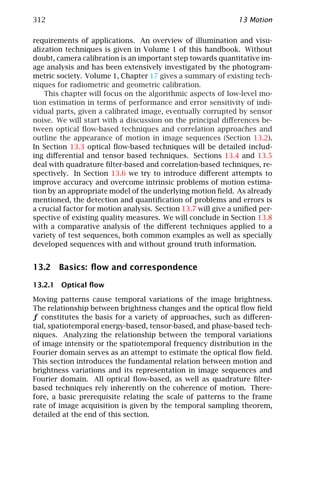
![13.2 Basics: flow and correspondence 313
Brightness change constraint. A common assumption on optical
flow is that the image brightness g(x, t) at a point x = [x, y]T at time t
should only change because of motion. Thus, the total time derivative,
dg ∂g dx ∂g dy ∂g
= + + (13.1)
dt ∂x dt ∂y dt ∂t
needs to equal zero. With the definitions f1 = dx/dt and f2 = dy/dt,
this directly yields the well-known motion constraint equation or bright-
ness change constraint equation, BCCE [10]:
( g)T f + gt = 0 (13.2)
T
where f = f1 , f2 is the optical flow, g defines the spatial gradient,
and gt denotes the partial time derivative ∂g/∂t.
This relation poses a single local constraint on the optical flow at a
certain point in the image. It is, however, ill-posed as Eq. (13.2) consti-
tutes only one equation of two unknowns. This problem is commonly
referred to as the aperture problem of motion estimation, illustrated in
Fig. 13.2a. All vectors along the constraint line defined by Eq. (13.2) are
likely to be the real optical flow f . Without further assumptions only
the flow f ⊥ ,
gt (x, t) g(x, t)
f ⊥ (x, t) = − n, n= (13.3)
g(x, t) g(x, t)
perpendicular to the constraint line can be estimated. This vector is
referred to as normal flow as it points normal to lines of constant image
brightness, parallel to the spatial gradient.
Although Eq. (13.2) is formulated for a single point in the image,
any discrete realization of the spatial and temporal derivatives requires
some neighborhood of the image point to be considered. From this fact,
the question arises, should the search for f be extended to a neighbor-
hood of finite size instead of focusing on a single point? If the spatial
gradient changes within this region, additional constraints can be used
to find the 2-D optical flow f . This is the common representation of the
aperture problem as illustrated in Fig. 13.2b and c. If the spatial struc-
ture within an aperture of finite size shows directional variations, the
optical flow f can be estimated unambiguously (Fig. 13.2b). In this case
the constraint lines of several points within the neighborhood have a
joint intersection. If, on the other hand, all gradient vectors within the
aperture are pointing into the same direction, all constraint lines fall
together and the aperture problem persists (Fig. 13.2c). A variety of
approaches have been proposed that directly use Eq. (13.2) by trying to
minimize an objective function pooling constraints over a small finite
area. They can be subdivided into differential techniques, using both
local and global constraints and tensor-based techniques (Section 13.3).](https://image.slidesharecdn.com/computervision-handbookofcomputervisionandapplicationsvolume2-signalprocessingandpatternrecognition-120205081400-phpapp02/85/Computer-vision-handbook-of-computer-vision-and-applications-volume-2-signal-processing-and-pattern-recognition-338-320.jpg)
![314 13 Motion
a
f2 b c
f
co
ns
tra f^
int
f^ lin
e
f1
Figure 13.2: Illustration of the aperture problem: a constraint line defined by
Eq. (13.2). The normal optical flow vector f ⊥ is pointing perpendicular to the
line and parallel to the local gradient g(x, t); b no aperture problem for local
neighborhoods with spatially distributed structures (moving corner); c within a
local neighborhood all gradients are parallel (moving edge). The optical flow
cannot be determined unambiguously.
In order to overcome the aperture problem, the size of the region of
interest has to be enlarged, as with the growing size of the local neigh-
borhood the chances for distributed spatial structure increase. At the
same time it becomes more likely that the region extends over motion
boundaries. These two competing obstacles of optical flow computa-
tion are referred to as the generalized aperture problem [11]. Recent
approaches to overcome this problem use robust statistics to avoid av-
eraging independent optical flow fields [12] (Section 13.6.2).
Optical flow in spatiotemporal images. In the previous section we
derived the brightness change constraint equation Eq. (13.2), relating
temporal and spatial derivatives of the image brightness to the optical
flow. Another basic relation can be found if we do not restrict the
analysis to two consecutive images but rather assume the brightness
pattern g(x, t) to be extended in both space and time, forming a 3-D
spatiotemporal image.
The displacement of brightness patterns within consecutive images
of a sequence yields inclined structures with respect to the temporal
axis of spatiotemporal images. Figure 13.3 shows examples of spa-
tiotemporal images for synthetic test patterns moving with constant
velocity.
T
Let r = [r1 , r2 , r3 ]T = a δx , δy , δt be the vector pointing into the
direction of constant brightness within the 3-D xt-domain. With δx
and δy we denote infinitesimal shifts of the brightness pattern within
the infinitesimal time step δt . The (arbitrary) scaling factor a will be
set to 1 in the remainder of this chapter, as only the fractions, r1 /r3
and r2 /r3 are relating r to the optical flow f . The relation between the
orientation angles, the spatiotemporal vector r, and the optical flow](https://image.slidesharecdn.com/computervision-handbookofcomputervisionandapplicationsvolume2-signalprocessingandpatternrecognition-120205081400-phpapp02/85/Computer-vision-handbook-of-computer-vision-and-applications-volume-2-signal-processing-and-pattern-recognition-339-320.jpg)
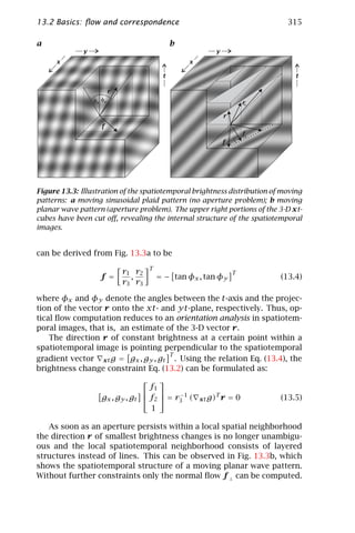
![316 13 Motion
It is important to note that Eqs. (13.2) and (13.5) are mathematically
equivalent and no constraint is added by extending the formulation of
the brightness conservation into 3-D space.
Motion constraint in Fourier domain. The concept of image sequences
as spatiotemporal images allows one to analyze motion in the corre-
sponding spatiotemporal frequency domain (Fourier domain).
Let g(x, t) be an image sequence of any pattern moving with con-
stant velocity, causing the optical flow f at any point in the image plane.
The resulting spatiotemporal structure can be described by
g(x, t) = g(x − f t) (13.6)
ˆ
The spatiotemporal Fourier transform g(k, ω) of Eq. (13.6) is given by
[13]
T
ˆ ˆ
g(k, ω) = g(k)δ(k f − ω) (13.7)
ˆ
where g(k) is the spatial Fourier transform of the pattern, and δ(·)
denotes Dirac’s delta distribution. Equation (13.7) states that the 3-D
Fourier spectrum of a pattern moving with constant velocity condenses
to a plane in Fourier space. The 2-D Fourier spectrum of the pattern is
being projected parallel to the temporal frequency ω onto the plane.
Figure 13.4a shows the spatiotemporal image of a 1-D random pattern
moving with 1 pixel/frame into positive x-direction. The corresponding
Fourier (power) spectrum is shown in Fig. 13.4b.
The equation of the plane in Fourier domain is given by the argument
of the delta distribution in Eq. (13.7):
T
ω(k, f ) = k f (13.8)
The normal vector of the plane is pointing parallel to the 3-D vec-
T
tor f1 , f2 , 1 . The plane constraint relation Eq. (13.8) is an equiv-
alent formulation of the brightness change constraint equation, BCCE
Eq. (13.2). It is the basis for all spatiotemporal energy-based techniques
(Section 13.4) that attempt to fit a plane to the Fourier spectrum of an
image sequence. From the inclination of the plane the optical flow can
be estimated. Taking the derivatives of ω(k, f ) Eq. (13.8) with respect
to kx and ky yields both components of the optical flow:
k ω(k, f ) =f (13.9)
The Fourier transform does not necessarily have to be applied to
the whole image. For local estimates, multiplication with an appropri-
ate window function prior to transformation restricts the spectrum to
a local neighborhood (Fig. 13.4c). It is, however, not possible to per-
form a Fourier transformation for a single pixel. The smaller the win-
dow, the more blurred the spectrum becomes [14] (compare Fig. 13.4b](https://image.slidesharecdn.com/computervision-handbookofcomputervisionandapplicationsvolume2-signalprocessingandpatternrecognition-120205081400-phpapp02/85/Computer-vision-handbook-of-computer-vision-and-applications-volume-2-signal-processing-and-pattern-recognition-341-320.jpg)
![13.2 Basics: flow and correspondence 317
a b
w
kx
t
x
c d
w
kx
t
x
Figure 13.4: Translating 1-D random pattern moving at 1 pixel/frame: a 2-
D xt-image (256 × 256); b power spectrum of the xt-image, with kx and ω
ranging from −π to π . The star-shaped patterns are due to the finite size of
the image; c windowed 2-D xt-image; d power spectrum of the windowed xt-
image.
with Fig. 13.4d). With the spatiotemporal window function w(x, t), the
resulting Fourier spectrum is blurred by the Fourier transform of w,
according to
ˆ ˆ
g · w(k, ω) = w(k, ω) ∗ [g(k)δ(kf − ω)] (13.10)
ˆ
where w(k, ω) denotes the Fourier transform of the window function
w(x, t), and ∗ defines the convolution
∞
a(k, ω) ∗ b(k, ω) = a(k − k , ω − ω )b(k , ω )dk dω (13.11)
−∞
Without additional windowing, w(x, t) is given by the size of the im-
age and the number of frames, that is, a box function with the size of
the spatiotemporal image. Its Fourier transform corresponds to a 2-
D sinc function, which can be observed in the star-shaped patterns of
Fig. 13.4b.
Hence, the Fourier domain formulation Eq. (13.8) intrinsically ex-
tends the motion constraint to a local neighborhood of a pixel. In case](https://image.slidesharecdn.com/computervision-handbookofcomputervisionandapplicationsvolume2-signalprocessingandpatternrecognition-120205081400-phpapp02/85/Computer-vision-handbook-of-computer-vision-and-applications-volume-2-signal-processing-and-pattern-recognition-342-320.jpg)
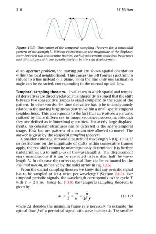
![13.2 Basics: flow and correspondence 319
the scale of a pattern, the more slowly it is allowed to move if the frame
rate cannot be increased. As all patterns can be decomposed into peri-
odic signals, Eq. (13.12) applies for any moving object. It is important
to note that it is not the size of the object, but rather the smallest wave
number contained in the Fourier spectrum of the object that is the limit-
ing factor. A large disk-shaped object can suffer from temporal aliasing
right at its edge, where high wave numbers are located.
If the temporal sampling theorem is violated by too large displace-
ments, temporal aliasing appears. In spatiotemporal images it shows
up as patterns with false inclinations or as distributed structures with-
out any relation at all. A prominent example of temporal aliasing is one
in which the wheels of horse-drawn carriages in movies seem to spin
around in the wrong direction.
An interesting analogy exists in the human visual system. From psy-
chophysical experiments with a random dot kinematogram [15] it was
found that human observers tend to estimate a coherent minimal mo-
tion, independent from the scale of clusters within the random pattern.
To explain these findings, Morgan [16] concludes that a coarse spatial
filter precedes motion detection in the human visual pathway [15].
Performing a low-pass filtering to remove all small scale spatial fre-
quencies beyond the critical limit is the basic idea of multiscale optical
flow computation techniques (Chapter 14). Starting from coarse pat-
terns, large displacements can be computed, which can be iteratively
refined from smaller scales. Such an approach, however, assumes that
patterns at all scales are moving with the same velocity. This is not
true for physical processes showing dispersion, such as water surface
waves.
It is important to note that the apparent motion, represented by the
optical flow field f , is the sampled motion, that is, the apparent mo-
tion after the spatiotemporal sampling process during image acquisi-
tion. If temporal aliasing persists, the real motion cannot be separated
from the apparently moving structures, unless other constraints apply.
Hence, optical flow computation or low level motion computation has to
be treated separately from higher level algorithms that attempt to solve
the problem of physical correspondence from visual correspondence.
13.2.2 Physical and visual correspondence
From the aperture problem we learned that only normal optical flow
can be computed in the case of linear symmetry of the brightness dis-
tribution within a local neighborhood. Translations parallel to lines of
constant gray values do not contribute to brightness variations and are
thus not detectable. The temporal sampling theorem states that large
displacements cannot be estimated from small-scale patterns. Both
problems of motion estimation can be considered as special cases of](https://image.slidesharecdn.com/computervision-handbookofcomputervisionandapplicationsvolume2-signalprocessingandpatternrecognition-120205081400-phpapp02/85/Computer-vision-handbook-of-computer-vision-and-applications-volume-2-signal-processing-and-pattern-recognition-344-320.jpg)
![320 13 Motion
a more general problem, commonly referred to as the correspondence
problem. The motion of patterns does not always allow for relating cor-
responding features in consecutive frames in an unambiguous manner.
The physical correspondence of features can remain undetectable due
to an aperture problem, missing texture (recall the example of the spin-
ning sphere in Fig. 13.1) or overly large displacements. Conversely, the
apparent motion can lead to false correspondence. Variation in scene
intensity may not be due to motion but instead may be caused by vari-
ations in illumination.
If local constraints are violated, correspondence-based techniques
try to estimate a best match of features within consecutive frames
(Chapter 13.5). Depending on the kind of features under considera-
tion, these techniques can be classified into correlation methods and
token tracking techniques [17]. Correlation techniques are computa-
tionally costly and therefore restricted to short-range displacements.
Token tracking methods extract features, such as corners, straight line
segments or blobs [18] and track them over time. The search can be
extended to the entire image area, which enables estimates of long-
range displacements. All correspondence-based techniques consider
only two single images. They do not use any information about the
continuous temporal domain.
13.2.3 Flow versus correspondence
There has been much discussion of the pros and cons of optical flow
based techniques in contrast to correspondence-based techniques. We
do not want to contribute to this dispute but rather recall which method
seems to be best suited under certain circumstances.
In order to solve the aperture problem a variety of optical flow-based
approaches have been proposed that try to minimize an objective func-
tion pooling constraints over a small finite area. An excellent overview
of the current state of the art is given by Barron et al. [6]. They conclude
that differential techniques, such as the local weighted least squares
method proposed by Lucas and Kanade [19] (Section 13.3.1), perform
best in terms of efficiency and accuracy. Phase-based methods [20]
(Section 13.4.3) show slightly better accuracy but are less efficient in im-
plementation and lack a single useful confidence measure. Bainbridge-
Smith and Lane [9] come to the same conclusion in their comparison of
the performance of differential methods. Performing analytical studies
of various motion estimation techniques, Jähne [21] and [13] showed
that the 3-D structure tensor technique (Section 13.3.2) yields the best
results with respect to systematic errors and noise sensitivity. This
could be verified by Jähne et al. [22], in their analysis of a calibrated
image sequence with ground truth data provided by Otte and Nagel [8].](https://image.slidesharecdn.com/computervision-handbookofcomputervisionandapplicationsvolume2-signalprocessingandpatternrecognition-120205081400-phpapp02/85/Computer-vision-handbook-of-computer-vision-and-applications-volume-2-signal-processing-and-pattern-recognition-345-320.jpg)
![13.3 Optical flow-based motion estimation 321
On the other hand, correspondence-based techniques (Section 13.5)
are less sensitive to illumination changes. They are also capable of es-
timating long-range displacements of distinct features that violate the
temporal sampling theorem. In this case any optical flow-based tech-
nique will fail. However, correlation-based approaches are extremely
sensitive to periodic structures. With nearly periodic inputs (such as
textures or bandpass filtered signals) they tend to find multiple local
minima [6]. Comparative studies show that correlation-based tech-
niques produce unpredictable output for straight edges (aperture prob-
lem), while optical-flow based techniques correctly estimate normal
flow. Correlation techniques also perform less effectively in estimat-
ing subpixel displacements than do optical flow-based techniques [6,
23]. Especially at very small displacements in the order of less than
1/10 pixel/frame, optical flow-based techniques yield better results.
Before we turn towards a detailed description of the various tech-
niques, we want to draw the conclusion that neither correlation nor
optical flow-based techniques are perfect choices in any case. If the
temporal sampling theorem can be assured to be fulfilled, optical flow-
based techniques are generally the better choice. In other cases, when
large displacements of small structures are expected, correlation-based
approaches usually perform better.
For both kind of techniques, it is important to get confidence mea-
sures in addition to the optical flow. No technique is without errors in
any case. Only if errors can be detected and quantified can the result
be reliably interpreted. It also shows that differences in precision, at-
tributable to details of the initial formulation, are, in fact, a result of
different minimization procedures and a careful numerical discretiza-
tion of the used filters.
13.3 Optical flow-based motion estimation
In this section we want to focus on common optical flow-based tech-
niques. We can not detail all facets of the spectrum of existing tech-
niques, but rather try to give a concise overview of the basic principles.
13.3.1 Differential techniques
Local weighted least squares. Assuming the optical flow f to be
constant within a small neighborhood U Lucas and Kanade [19] propose
a local weighted least squares estimate of the constraint Equation (13.2)
on individual pixels within U. Similar approaches are reported by [24,
25, 26, 27]. The estimated optical flow is given by the solution of the](https://image.slidesharecdn.com/computervision-handbookofcomputervisionandapplicationsvolume2-signalprocessingandpatternrecognition-120205081400-phpapp02/85/Computer-vision-handbook-of-computer-vision-and-applications-volume-2-signal-processing-and-pattern-recognition-346-320.jpg)
![322 13 Motion
following minimization problem:
∞
2
2 2
f = arg min e 2, e 2 = w(x − x ) ( g)T f + gt dx (13.13)
−∞
with a weighting function w(x) selecting the size of the neighborhood.
In practical implementations the weighting is realized by a Gaussian
smoothing kernel. Additionally, w could weight each pixel according
to some kind of confidence measure, for example, the magnitude of
the gradient. In that way, a priori known errors are not propagated into
the optical flow computation.
In the initial formulation of [19], Eq. (13.13) was given by a discrete
sum of the squared residuals ( g)T f + gt , which have to be minimized.
The mathematically equivalent continuous least squares formulation
Eq. (13.13) replaces the weighted sum by a convolution integral [13, 21].
This formulation enables us to use linear filter theory, which allows, for
example, optimizing the convolution kernels independently from the
minimization procedure. In this way practical implementations of dif-
ferent approaches can be quantitatively compared without confusing
discretization errors with intrinsic errors of the algorithms.
The minimization of Eq. (13.13) is carried out by standard least
squares estimation. Both partial derivatives of e 2 with respect to
2
the two components f1 and f2 of the optical flow f have to equal zero
at the minimum of e 2 : 2
∞
∂ e 22 !
=2 w(x − x )gx ( g)T f + gt dx = 0 (13.14)
∂f1
−∞
∞
∂ e 22 !
=2 w(x − x )gy ( g)T f + gt dx = 0 (13.15)
∂f2
−∞
If the optical flow f is assumed to be constant within the area of influ-
ence of w, it can be drawn out of the integral. Combining Eq. (13.14)
and Eq. (13.15) yields the following linear equation system
g x gx gx gy f1 g x gt
=− (13.16)
gx gy gy gy f2 gy gt
A f b
with the abbreviation
∞
a = w(x − x ) a dx (13.17)
−∞](https://image.slidesharecdn.com/computervision-handbookofcomputervisionandapplicationsvolume2-signalprocessingandpatternrecognition-120205081400-phpapp02/85/Computer-vision-handbook-of-computer-vision-and-applications-volume-2-signal-processing-and-pattern-recognition-347-320.jpg)
![13.3 Optical flow-based motion estimation 323
In operator notation, the components of Eq. (13.16) are given by
gp gq = B(Dp · Dq ), and gp gt = B(Dp · Dt ) (13.18)
where B is a smoothing operator and Dp , Dq , and Dt are discrete first-
order derivative operators in the spatial directions p and q and in time
direction t, respectively. The solution of Eq. (13.16) is given by
f = A−1 b (13.19)
provided the inverse of A exists. If all gradient vectors within U are
pointing into the same direction, A gets singular. Then, the brightness
distribution can be expressed locally as
T
g(x) = g(d x) (13.20)
T
where d = [d1 , d2 ] is a vector pointing perpendicular to lines of con-
stant brightness. From Eq. (13.20) the first-order partial derivatives
can be computed as gx = d1 g and gy = d2 g , where the abbreviation
T
g = ∂g/∂(d x) is used. The determinant
2
det (A) = gx gx gy gy − gx gy (13.21)
equals zero and A cannot be inverted. Thus, averaging Eq. (13.2) over
a small neighborhood does not yield more information than a single
point if the aperture problem persists within the neighborhood. In this
case, only the normal flow f ⊥ is computed according to Eq. (13.3).
Instead of zero determinant, singularity of A can be identified by an-
alyzing the eigenvalues of the symmetric matrix A prior to inversion.
While Simoncelli [27] suggests using the sum of eigenvalues, Barron
et al. [6] conclude that the smallest eigenvalue constitutes a more reli-
able measure. In Section 13.7 we will compare common confidence and
type measures of different approaches and show how they are related.
Jähne [13] shows that an extension of the integration in Eq. (13.13)
into the temporal domain yields a better local regularization, provided
that the optical flow is modeled constant within the spatiotemporal
neighborhood U. However, this does not change the minimization pro-
cedure and results in the same linear equation system Eq. (13.16). All
that needs to be changed are the components a
∞
a = w(x − x , t − t ) a dx dt (13.22)
−∞
where both the integration as well as the window function w have been
extended into the temporal domain.
While the presence of an aperture problem can be identified by the
singularity of the matrix A, the initial assumption of constant optical](https://image.slidesharecdn.com/computervision-handbookofcomputervisionandapplicationsvolume2-signalprocessingandpatternrecognition-120205081400-phpapp02/85/Computer-vision-handbook-of-computer-vision-and-applications-volume-2-signal-processing-and-pattern-recognition-348-320.jpg)
![324 13 Motion
flow within U remains to be proved. In any case, an averaged optical
flow will be computed by the solution of Eq. (13.19). This leads to
over-smoothing of the optical flow field at motion discontinuities and
false estimation at the presence of transparent motion overlay. Such
cases lead to nonzero values of the expression ( g)T f + gt , which
is called the measurement innovation, or the residual. The residual
reflects the discrepancy between the predicted measurement ( g)T f
and the actual measurement gt . A residual of zero means that both are
in complete agreement. Thus, a nonconstant optical flow field can be
detected by analyzing the variance of the data σ 2 , given by the squared
magnitude of the residuals [13]
2
2
σ2 = e 2 = ( g)T f + gt (13.23)
where f is the estimated optical flow. In case of constant f within
U, the residuals in Eq. (13.23) vanish and σ 2 reduces to the variance
cause by noise in the image. Thus, a variance significantly larger than
the noise variance is a clear indicator for a violation of the assumption
of constant optical flow. In real applications, f will never be constant
over the whole image. If it varies smoothly over the image area, it can be
considered locally constant and the local least squares estimate can be
applied. Other models of the spatial distribution of f (x), such as linear
(affine) motion, can be incorporated into the least squares approach as
well. This will be the subject of Section 13.6.1.
From a probabilistic point of view, the minimization of Eq. (13.13)
corresponds to a maximum likelihood estimation of the optical flow,
given Gaussian-distributed errors at individual pixels [28]. Black and
Anandan [12] show that the Gaussian assumption does not hold for
motion discontinuities and transparent motions. By replacing the least
squares estimation with robust statistics they come up with an iterative
estimation of multiple motions (Section 13.6.2).
Second-order techniques. Instead of grouping constraints over a lo-
cal neighborhood, it has been proposed to use second-order informa-
tion to solve for both components of f [29, 30, 31]. This can be moti-
vated by extending the brightness constancy assumption to an assump-
tion on the conservation of the gradient g under translation:
d( g)
=0 (13.24)
dt
Evaluating Eq. (13.24) yields the following linear equation system for a
single point:
gxx gxy f1 gtx
=− (13.25)
gxy gyy f2 gty
H f b](https://image.slidesharecdn.com/computervision-handbookofcomputervisionandapplicationsvolume2-signalprocessingandpatternrecognition-120205081400-phpapp02/85/Computer-vision-handbook-of-computer-vision-and-applications-volume-2-signal-processing-and-pattern-recognition-349-320.jpg)
![13.3 Optical flow-based motion estimation 325
The matrix H is the Hessian of the image brightness function, con-
taining all second-order partial spatial derivatives gpq = ∂ 2 g/∂p∂q.
The second-order spatiotemporal derivatives in b are abbreviated by
gtp = ∂ 2 g/∂t∂p. The linear equation system Eq. (13.25) can be solved
by
f = H −1 b (13.26)
if the Hessian matrix is not singular. This happens if the determinant
vanishes,
2
det (H) = gxx gyy − gxy = 0 (13.27)
The trivial solution of Eq. (13.27) is given for vanishing second-order
derivatives, gxx = gyy = gxy = 0, that is, local planar brightness distri-
bution. Equation (13.27) also holds, if the image brightness shows lin-
ear symmetry within the local area supporting the second-order deriva-
tive operators. In this case, the brightness distribution can be ex-
pressed locally as
T
g(x) = g(d x) (13.28)
T
where d = [d1 , d2 ] is a vector pointing perpendicular to lines of con-
stant brightness. From Eq. (13.28) the second-order partial derivatives
can be computed as
gxx = d2 g ,
1 gyy = d2 g ,
2 and gxy = d1 d2 g (13.29)
T
where the abbreviation g = ∂ 2 g/∂(d x)2 is used. With Eq. (13.29) the
condition Eq. (13.27) is satisfied and the Hessian H cannot be inverted.
Thus, second-order techniques, just as first-order techniques, do
not allow for estimating the 2-D optical flow field f in case of an aper-
ture problem within a local neighborhood. Although no local averaging
has been performed to obtain the solution Eq. (13.25), a local neighbor-
hood is introduced by the region of support of the second-order deriva-
tive operators. In order to obtain second-order differential information,
first-order properties of the image area need to be related over an in-
creased area compared to first-order differentiation. From first-order
information the full 2-D optical flow can only be extracted if the spatial
orientation changes within the region of interest. Bainbridge-Smith and
Lane [9] conclude that first-order differential techniques, such as pro-
posed by Lucas and Kanade [19], are in fact generalized second-order
techniques, because they implicitly require variation of the gradient
within the region of support.
The initial assumption (Eq. (13.24)) requests that first-order (affine)
motions, such as dilation, rotation or shear, are not allowed in the op-
tical flow field. This constraint is much stronger than the brightness](https://image.slidesharecdn.com/computervision-handbookofcomputervisionandapplicationsvolume2-signalprocessingandpatternrecognition-120205081400-phpapp02/85/Computer-vision-handbook-of-computer-vision-and-applications-volume-2-signal-processing-and-pattern-recognition-350-320.jpg)
![326 13 Motion
conservation assumption of Eq. (13.2) and is fulfilled only rarely for
real motion fields. Hence, second-order techniques generally lead to
sparser optical flow fields than those of first-order techniques [6]. If
the assumption of conserved gradient is violated, the residual error
2 2
e 2 = [Hf − b] (13.30)
will increase beyond the noise variance σ 2 (compare to Eq. (13.23)),
which allows one to identify erroneous estimates of f .
Global constraints. Local least squares techniques minimize the
brightness change constraint equation Eq. (13.2) over a localized aper-
ture, defined by the size of the spatial window function w (Eq. (13.13)).
Global constraint methods extend the integration to the entire image
area and combine the local gradient constraint Eq. (13.2) with a spatial
coherence assumption. The resulting objective function e t 2 to be
2
minimized consists of two terms. The first one, e d 2 , contains the
2
local data (brightness) conservation constraint Eq. (13.2) at each pixel
and a second one, e s 2 , expresses the spatial relation between optical
2
flow vectors:
2
2 2 2 2
et 2 = ed 2 + λ2 e s 2 = ( g)T f + gt dx + λ2 e s 2 (13.31)
D
The integration is carried out over the domain D, which can be extended
to the entire image. The parameter λ controls the influence of the spa-
tial coherence term. The optical flow f is estimated by minimizing
et 2 ,
2
2
f = arg min e t 2 (13.32)
The introduction of a regularizing spatial coherence constraint e s 2 2
restricts the class of admissible solutions and makes the problem well-
posed [12]. A variety of approaches have been proposed in the liter-
ature, dealing with the choice of an appropriate spatial constraint. In
general, it should interpolate optical flow estimates at regions suffering
from the aperture problem or without sufficient brightness variations.
At the same time spatial oversmoothing of motion boundaries should
be prevented. Both are competing requirements.
The most common formulation of e s 2 has been introduced by
2
Horn and Schunk [10]. They propose a global smoothness constraint of
the form
2 2 2 2
2 ∂f1 ∂f1 ∂f2 ∂f2
es 2 = + + + dx (13.33)
∂x ∂y ∂x ∂y
D](https://image.slidesharecdn.com/computervision-handbookofcomputervisionandapplicationsvolume2-signalprocessingandpatternrecognition-120205081400-phpapp02/85/Computer-vision-handbook-of-computer-vision-and-applications-volume-2-signal-processing-and-pattern-recognition-351-320.jpg)
![13.3 Optical flow-based motion estimation 327
Minimizing Eq. (13.32) by means of Gauss-Seidel iteration [32] yields an
(k+1)
iterative solution for the optical flow f at time step k + 1 given the
(k)
flow f at time k:
(k)
(k+1) (k)
g f + gt
f = f − g 2
(13.34)
g 2 + λ2
(k) (k) (0)
where f denotes a local average of f . The initial estimate f
is usually set to zero for the entire image. It is important to note that
the gradient g apparently controls the influence of both terms in
Eq. (13.34). If the gradient vanishes, that is, at regions with low spatial
structure, the optical flow is interpolated from adjacent estimates. In
regions with high contrast the local brightness change constraint (nu-
merator of the right term in Eq. (13.34)) becomes dominant.
The propagation of the flow field into regions with low contrast is
an important feature of Horn and Schunck’s smoothness constraint.
However, as no directional selectivity is included in Eq. (13.33) the re-
sulting flow field is blurred over motion discontinuities. It also has
the drawback that a localized error can have a far-reaching effect if the
surrounding gradients are small [9].
In order to reduce smoothing across edges, Nagel [29, 33, 34] sug-
gests an oriented smoothness constraint:
2 1
es 2 = 2 [E1 + δE2 ] dx (13.35)
g 2 + 2δ
D
2 2
∂f1 ∂f1 ∂f2 ∂f2
E1 = gy − gx + gy − gx (13.36)
∂x ∂y ∂x ∂y
2 2 2 2
∂f1 ∂f1 ∂f2 ∂f2
E2 = + + + (13.37)
∂x ∂y ∂x ∂y
The additional parameter δ controls the relative influence of the ori-
ented smoothness term E1 compared to E2 , which constitutes Horn and
Schunck’s global smoothness constraint. Again, the solution is given by
an iterative Gauss-Seidel method. As an interesting feature, the rather
complicated solution equations implicitly contain second-order deriva-
tives.
In a more restrictive way, Hildreth [35, 36] reduce all computations
to zero crossings of a Laplace-filtered image. Along these contour lines
C, an objective function is defined according to
2 2
2
2 ∂f1 ∂f2
et 2 = ( g)T f + gt + λ2 + ds (13.38)
∂s ∂s
C](https://image.slidesharecdn.com/computervision-handbookofcomputervisionandapplicationsvolume2-signalprocessingandpatternrecognition-120205081400-phpapp02/85/Computer-vision-handbook-of-computer-vision-and-applications-volume-2-signal-processing-and-pattern-recognition-352-320.jpg)
![328 13 Motion
where the first term in the integral is given by the standard data conser-
vation constraint Eq. (13.31) and ∂fp /∂s, denotes the directional deriva-
tive of fp into the direction s along the contour C. In contrast to other
approaches, all integrations are carried out along contour lines instead
of by 2-D averaging. Thus, no information is smoothed across bright-
ness edges. However, the approach inherently assumes that all edges
belong to the same object. If contours of independently moving objects
merge, the resulting optical flow field is blurred along the contour line
as well.
All approaches incorporating global constraints have in common
that they result in systems of differential equations relating spatial vari-
ations of the optical flow within the entire domain D. Such a system can
only be solved iteratively using numerical iteration methods, such as
Gauss-Seidel iteration or successive overrelaxation [28, 37]. Although
efficient iterative solutions have been developed in numerical mathe-
matics, they are still slower than closed solutions. Another problem of
iterative solutions is the question of convergence, which may depend on
image content. Further information on global constraints can be found
in Chapter 16, where a general toolbox for variational approaches is
proposed, together with an efficient numerical iteration scheme.
13.3.2 Tensor-based techniques
In Section 13.2.1 we have shown that optical flow computation can be
formulated as orientation analysis in spatiotemporal images. A prac-
tical example of such a spatiotemporal image and the corresponding
structures is shown in Fig. 13.6. This application example has been
chosen for illustration because it demonstrates nicely how any mov-
ing gray-value structure causes inclined patterns, regardless of certain
object properties.
In order to determine local orientation Bigün and Granlund [38] pro-
posed a tensor representation of the local image brightness distribution.
Starting with a different idea, Kass and Witkin [39] came to a solution
that turned out to be equivalent to the tensor method. Searching for
a general description of local orientation in multidimensional images,
Knutsson [40, 41] concluded that local structure in an n-dimensional
domain can be represented by a symmetric n × n tensor of second-
order. In the analysis of data with a dimensionality higher than two it
turns out that using scalars and vectors is no longer always convenient
[42]. Tensors—a generalization of the vector concept—are perfectly
suited to describe symmetries within local neighborhoods in multidi-
mensional spatial and spatiotemporal signals.
This section outlines the practical application of tensor representa-
tions to optical flow computation and its relation to other optical flow-
based techniques. We will show how a local least squares estimation](https://image.slidesharecdn.com/computervision-handbookofcomputervisionandapplicationsvolume2-signalprocessingandpatternrecognition-120205081400-phpapp02/85/Computer-vision-handbook-of-computer-vision-and-applications-volume-2-signal-processing-and-pattern-recognition-353-320.jpg)
![13.3 Optical flow-based motion estimation 329
Figure 13.6: Illustration of the spatiotemporal brightness distribution of moving
patterns. The sequence shows infrared images of the ocean surface moving
mainly in positive x-direction. The upper right portion of the 3-D xt- cube has
been cut off, revealing the internal structure of the spatiotemporal image.
of optical flow, such as the approach of Lucas and Kanade [19], can be
improved by using total least squares estimation instead of standard
least squares. This leads directly to the structure tensor technique for
optical flow computation [43, 44, 45, 46], which constitutes the most di-
rect approach to linear symmetry detection in spatiotemporal images.
Another tensor representation, based on combinations of quadrature
filters, will be outlined in Section 13.4.2.
The structure tensor approach. The optical flow f and the direction
r of constant brightness within a spatiotemporal image are related by
f = r3 1 [r1 , r2 ]T (Eq. (13.4)). Within a local neighborhood U, the vector
−
r has to be as perpendicular as possible to the spatiotemporal gradient
T
xt g = gx , gy , gt . Thus, the scalar product ( xt g)T r has to vanish
at any point within U for the optimum estimate of r (Eq. (13.5)). In a
least squares sense, r can be found by minimizing
∞
2
2 2 T
r = arg min e 2, e 2 = w(x − x ) ( xt g) r dx (13.39)
r T r =1
−∞
which is equivalent to Eq. (13.13). In order to avoid the trivial solution
r = 0, the constraint r T r = 1 has to be imposed on r. The information
within a local neighborhood U around the central point x = [x, y, t]T
is weighted by a window–function w(x − x ). In practical applications
the size of the local neighborhood U represents the area over which
the optical flow is averaged. Again, the spatial integration can be ex-
tended into the time domain for local regularization without changing
the results of the following minimization procedure [13].](https://image.slidesharecdn.com/computervision-handbookofcomputervisionandapplicationsvolume2-signalprocessingandpatternrecognition-120205081400-phpapp02/85/Computer-vision-handbook-of-computer-vision-and-applications-volume-2-signal-processing-and-pattern-recognition-354-320.jpg)
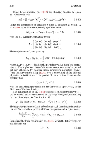
![13.3 Optical flow-based motion estimation 331
Thus, the minimization reduces to an eigenvalue problem of the sym-
metric matrix J. Once a minimizing r is found, Eq. (13.41) reduces
to
2
e 2 = r T J r = r T λr = λ (13.48)
which shows that the minimum of Eq. (13.41) is reached if the vector r
is given by the eigenvector of the tensor J to the minimum eigenvalue
λ.
Total least squares versus standard least squares. Although the
local least squares technique (Eq. (13.13)) and the structure tensor tech-
nique (Eq. (13.39)) are based on the same initial formulation, the corre-
sponding solutions Eqs. (13.19) and (13.47) are quite different. Practical
implementations of both techniques also show that the structure tensor
technique is more accurate (Section 13.8). Performing analytical stud-
ies Jähne [13] showed that the local least squares technique is biased
towards lower values of f in the presence of noise, while the structure
tensor technique yields an unbiased estimate for isotropic noise. What
are the basic differences of both techniques and how are they related?
In order to answer this question we have to examine the minimization
procedure of Eqs. (13.13) and (13.39), respectively.
In a discrete formulation, both problems of local optical flow esti-
mation constitute linear equation systems of the form
gx (x 1 ) gy (x 1 ) gt (x 1 )
gx (x 2 ) gy (x 2 ) f gt (x 2 )
1
. . = − . (13.49)
.
. .
. f2 .
.
gx (x N ) gy (x N ) gt (x N )
X f y
for N points within the local neighborhood U. The weighting coeffi-
cients w(x i ) have been set to unity in order to simplify the notation.
However, this does not affect the algebraic relations of the following
argumentation.
The task of optical flow estimation can be formulated in the fol-
lowing way: given a set of explanatory variables g(x i ) (data matrix
X) and a set of response variables gt (x i ) (vector of observations y),
try to find a best estimate of the true but unknown model parameters
T
f = f1 , f2 , which are assumed to be constant within U. If Eq. (13.49)
is overdetermined (N > 2), only approximate solutions can be found
using either a standard least squares (LS) or a total least squares (TLS)
approach. An excellent overview of the total least squares problem and
practical applications can be found in [47].](https://image.slidesharecdn.com/computervision-handbookofcomputervisionandapplicationsvolume2-signalprocessingandpatternrecognition-120205081400-phpapp02/85/Computer-vision-handbook-of-computer-vision-and-applications-volume-2-signal-processing-and-pattern-recognition-356-320.jpg)
![332 13 Motion
Least squares The classical least squares (LS) approach assumes the
explanatory variables of the data matrix X to be free of error, that
is, measured with infinite precision. All errors are confined to the
observation vector y. To find the model parameter f , the least
squares estimate seeks to
2
min y − y 2, y = Xf (13.50)
by searching for a minimizing f . In minimizing Eq. (13.50) the gra-
dients g(x i ) and the temporal derivatives gt (x i ) are treated sep-
arately. A best estimate f is found by taking the derivatives of the
quadratic objective function y − y 2 —which can be considered,
2
as squared magnitude of a 2-D residual error vector —with respect
to the two components f1 and f2 .
Total least squares The total least squares (TLS) approach is motivated
by the fact that errors due to sampling and noise may imply inaccu-
racies of the data matrix X as well. In the case of motion estimation
both spatial and temporal derivatives may be corrupted. This fact
can be accounted for by combining X and y to the augmented data
matrix C
gx (x 1 ) gy (x 1 ) gt (x 1 )
gx (x 2 ) gy (x 2 ) gt (x 2 )
C = [X; y] = . . . (13.51)
.
. .
. .
.
gx (x N ) gy (x N ) gt (x N )
With Eq. (13.51) the linear equation system Eq. (13.49) reduces to
T T
[X; y] f ; 1 = r3 1 Cr = 0
−
(13.52)
where the 3-D vector r is defined in Eq. (13.4). In order to find a best
estimate of r, we seek to
2
min Cr 2, subject to r T r = 1 (13.53)
where the quadratic constraint r T r = 1 is added to avoid the trivial
solution r = 0. In minimizing Eq. (13.53), the gradients g(x i ) and
the temporal derivatives gt (x i ) are treated on an equal basis. A best
estimate for r is found by taking the derivatives of the quadratic ob-
jective function Cr 2 —which can be considered as squared mag-
2
nitude of a 3-D residual error vector —with respect to all three com-
ponents r1 , r2 , and r3 . This method of obtaining a linear relation
between the columns of a matrix C is known as linear orthogonal
l2 approximation [48, 49], which is an alternative formulation of the
total least squares estimation problem [47, 50].](https://image.slidesharecdn.com/computervision-handbookofcomputervisionandapplicationsvolume2-signalprocessingandpatternrecognition-120205081400-phpapp02/85/Computer-vision-handbook-of-computer-vision-and-applications-volume-2-signal-processing-and-pattern-recognition-357-320.jpg)
![13.3 Optical flow-based motion estimation 333
a b
least squares (LS) total least squares (TLS)
yi yi 2σx
2σy 2σy
error error
distribution distribution
xi xi
Figure 13.7: Illustration of the difference between a standard least squares (LS)
and b total least squares (TLS) estimation. Errors in the measured variables are
indicated by Gaussian distributions. While LS assumes errors to be confined to
the observables yi , TLS allows errors in the variables xi as well.
The basic difference of least squares and total least squares can
be illustrated by a simple regression problem fitting a straight line to
measurements. Standard least squares minimizes the vertical deviation
of the response variables to the estimated line, while total least squares
minimizes the Euclidean distances of the points to the line (Fig. 13.7).
In terms of optical flow computation, using TLS instead of LS esti-
mation implies two important differences on the results of either tech-
nique:
• Instead of only the two parameters f1 and f2 , the total least squares
technique varies all three parameters of the vector r. This leads to
a robust estimate of the spatiotemporal orientation in contrast to a
fixed temporal component using standard least squares.
• Both techniques yield matrices with components of the form gp gq ,
where gp denotes partial derivatives in x, y, and t. Comparing the
structure tensor Eq. (13.42) to the least squares solution Eq. (13.16)
shows that the purely temporal component gt gt of Eq. (13.42) is
missing in Eq. (13.16). This component, however, allows to sepa-
rate isotropic noise, occlusions, and fast accelerations from coher-
ent motion as shown in the following section. Such regions violating
the model assumption of constant f within U have to be detected
by analyzing the residual errors in the standard least squares esti-
mation.
As a conclusion we note that the difference between the local least
squares method of Lucas and Kanade [19] and the structure tensor for-
mulation is neither imposed by the formulation of the minimization
problem nor by the extension into the temporal domain, but rather by
the minimization procedure.](https://image.slidesharecdn.com/computervision-handbookofcomputervisionandapplicationsvolume2-signalprocessingandpatternrecognition-120205081400-phpapp02/85/Computer-vision-handbook-of-computer-vision-and-applications-volume-2-signal-processing-and-pattern-recognition-358-320.jpg)
![334 13 Motion
Most recently, a number of authors have become aware of the sub-
tle difference between the two minimization procedures, which leads to
significant differences in the accuracy of a variety of optical flow tech-
niques [51, 52]. An interesting extension of the TLS technique, referred
to as extended least squares technique (ELS), was proposed by Srinivasan
and Chellappa [52]. They show that the TLS optical flow solution is un-
biased only if the error in estimating the temporal gradient is equal in
variance to the error in estimating the spatial gradient. This, however,
cannot always be satisfied, for example, if spatial and temporal deriva-
tive operators have different extensions. Using the ELS solution, this
bias can be avoided.
All least squares techniques, however, intrinsically assume that the
errors are Gaussian and independent with constant variance for all
points within U [32]. This prerequisite leads directly to the quadratic
form of the error function of either technique. The assumption of Gaus-
sian error distributions is violated for multiple motions within U. In
this case, quadratic objective functions tend to over-weight outliers,
which can be reduced using robust error norms [12] (Section 13.6.2).
Eigenvalue analysis. In order to estimate optical flow from the struc-
ture tensor J we need to carry out an eigenvalue analysis of the sym-
metric 3×3 tensor (Eq. (13.47)). The symmetry of J implies that all three
eigenvalues are real and it further implies that there is an orthonormal
basis of eigenvectors [37]. These vectors are pointing into the direc-
tions of minimal and maximal brightness changes, respectively, span-
ning the principal-axes coordinate system of the local 3-D spatiotem-
poral neighborhood U. In the principal-axes system, the transformed
structure tensor J is diagonal and contains the eigenvalues of J as
diagonal elements:
λ1 0 0
J = 0 λ2 0 (13.54)
0 0 λ3
Without restricting generality, the eigenvalues are sorted in descending
order:
λ1 ≥ λ2 ≥ λ3 ≥ 0 (13.55)
and the corresponding eigenvectors are denoted by r 1 , r 2 , and r 3 .
Eigenvalue analysis is a nontrivial but standard problem of numer-
ical linear algebra for which a number of efficient solutions have been
developed [28, 37]. A standard procedure in numerical eigenvalue anal-
ysis is the Jacobi method. It consists of a sequence of orthogonal simi-
larity transformations designed successively to annihilate off-diagonal
elements of the matrix. The Jacobi method is absolutely foolproof for
all real symmetric matrices, such as the structure tensor (regardless of
the image content).](https://image.slidesharecdn.com/computervision-handbookofcomputervisionandapplicationsvolume2-signalprocessingandpatternrecognition-120205081400-phpapp02/85/Computer-vision-handbook-of-computer-vision-and-applications-volume-2-signal-processing-and-pattern-recognition-359-320.jpg)
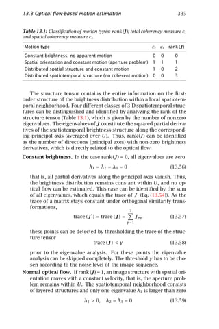
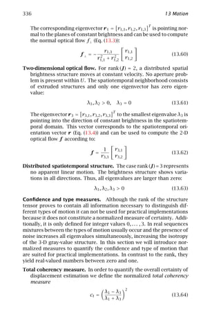
![13.3 Optical flow-based motion estimation 337
with λ1 and λ3 denoting the largest and smallest eigenvalue of the
structure tensor, respectively. Table 13.1 shows the values of ct
for different cases of motion. For both types of apparent motion,
that is, aperture problem and no aperture problem, ct equals one.
If no displacement can be computed it is identical to zero. With
increasing noise level ct approaches zero for all different types of
motion.
Spatial coherency measure. While the total coherency ct gives a nor-
malized estimate for the certainty of local spatiotemporal orienta-
tion it does not allow identification of areas of apparent aperture
problem. In order to quantify the presence of an aperture problem
we define the spatial coherency measure (edge measure)
2
λ 1 − λ2
cs = (13.65)
λ1 + λ2
where λ2 denotes the second largest eigenvalue of the structure ten-
sor. Table 13.1 shows the values of cs for different cases of motion.
Only if an aperture problem is present does cs reach its maximum
value of ct . For all other types of motion it equals zero. The spatial
coherency measure can be identified as the coherency measure of 2-
D local orientation estimation (Volume 2, Section 10.6.7, Eq. (10.74)).
Note that cs is normalized between zero and ct because it is not pos-
sible to detect the presence of an aperture problem more reliably
than the overall certainty.
Corner measure. From the two independent measures ct and cs , a third
number, which can be referred to as corner measure cc , can be com-
puted by cc = ct −cs . It constitutes the counterpart of cs , quantifying
the absence of an aperture problem, that is, selecting points where
both components f1 and f2 of the optical flow f can be reliably
computed.
Figure 13.8 illustrates the coherency and type measures for a mov-
ing calibration target on a linear positioning table. The coherency mea-
sure shows the entire grid without regions of homogeneous brightness.
These areas split up into the edges and crossing points of the grid for
the edge and corner measure, respectively.
The importance of confidence and type measures for quantitative
image sequence analysis are illustrated in Fig. 13.9 for a moving ring
pattern with additive noise. The optical flow field shows random flow
vectors in regions with homogeneous brightness. With the total co-
herency measure these regions can be identified. Further knowledge
about the presence of an aperture problem allows reconstruction of
the 2-D flow field from normal flow, using the local regularization tech-
nique outlined in the following section [44]. It has to be pointed out](https://image.slidesharecdn.com/computervision-handbookofcomputervisionandapplicationsvolume2-signalprocessingandpatternrecognition-120205081400-phpapp02/85/Computer-vision-handbook-of-computer-vision-and-applications-volume-2-signal-processing-and-pattern-recognition-362-320.jpg)
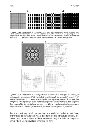
![13.3 Optical flow-based motion estimation 339
Two-dimensional flow from normal flow. For all image points with
high values of the total coherency measure and simultaneously low
values of the spatial coherency measure, that is, (ct − cs ) ≈ ct ≈ 1,
the 2-D optical flow f can be computed according to Eq. (13.62). But
how do we treat points suffering from the aperture problem, that is,
cs ≈ ct ≈ 1?
It is important to note that an aperture problem does not introduce
an erroneous optical flow field but only allows computation of partial
information, eventually with high precision. As another important fact,
more edge-like structures are statistically contained in images than iso-
lated points or corners. Hence, it would be too much of a restriction
to throw away all aperture problem pixels. On the other hand, long
and straight lines are also less likely than slightly curved structures.
Thus, it should be possible to reliably compute normal flow at edges
and group it over an enlarged neighborhood to estimate the 2-D optical
flow. The two measures cs and ct quantify the presence of an aperture
problem as well as a certainty of the corresponding normal flow vector
f ⊥ . Given this information and the previously computed normal flow
f ⊥ , we try to find a best estimate of the 2-D optical flow f .
For any point suffering from the aperture problem, the normal flow
f ⊥ is related to the optical flow f by
T g
ˆ
f ⊥ = f n, ˆ
n= (13.66)
g
where n = [n1 , n2 ]T denotes a unit vector normal to lines of constant
ˆ
brightness in the image, that is, perpendicular to edges. The normal
vector can be computed directly from the eigenvector of the structure
T
tensor to the largest eigenvalue, r 1 = r1,1 , r1,2 , r1,3 , by
2 2
−1/2 r1,1
ˆ
n = r1,1 + r1,2 (13.67)
r1,2
using solely the spatial components of r 1 .
Similar to the local least squares approach of Lucas and Kanade
[19], the search for a best estimate of f can be extended to a slightly
larger neighborhood, U > U, where U denotes the area of support of
the smoothing kernel w used for the initial estimate of normal flow in
Eq. (13.39) [44].
A local least squares estimate of f can be found by minimizing the
following objective function with respect to both components f1 and
f2 :
2
f = arg min e 2 (13.68)
with](https://image.slidesharecdn.com/computervision-handbookofcomputervisionandapplicationsvolume2-signalprocessingandpatternrecognition-120205081400-phpapp02/85/Computer-vision-handbook-of-computer-vision-and-applications-volume-2-signal-processing-and-pattern-recognition-364-320.jpg)
![340 13 Motion
∞
T 2
2 −1
e 2 = c ˆ
w(x − x )c(x ) f n(x ) − f⊥ (x ) dx (13.69)
−∞
and
∞
c = w(x − x )c(x ) dx (13.70)
−∞
The size of the local neighborhood is defined by a window function
w, which can be chosen independently from the one in Eq. (13.39).
The measure c incorporates any confidence measure, such as, for ex-
ample, binary masks obtained by thresholding ct and cs , or analytical
functions of ct and cs . Unequal weighting of individual pixels due to
distributed confidence within U formally requires a normalization of
the objective function, given by c −1 . This corresponds to a normal-
ized convolution, introduced by Granlund and Knutsson [42]. However,
c −1 constitutes a constant within U that does not propagate into the
following minimization procedure and, therefore, can be omitted in the
practical implementation.
Solving Eq. (13.68) by standard least squares technique yields the
linear equation system
cn1 n1 cn1 n2 f1 cn1 f⊥
= (13.71)
cn1 n2 cn2 n2 f2 cn2 f⊥
A f b
with
∞
cnp nq = w(x − x )c(x )np (x )nq (x ) dx (13.72)
−∞
and
∞
cnp f⊥ = w(x − x )c(x )np (x )f⊥ (x ) dx (13.73)
−∞
Equation (13.71) has a solution if the Matrix A can be inverted, which
is the case only if
2
det (A) = cn1 n1 cn2 n2 − cn1 n2 ≠0 (13.74)
If all normal vectors within U are collinear, det (A) = 0. In this case the
aperture problem remains within U and Eq. (13.71) does not yield more
ˆ
information than a single value of f⊥ . As the vectors n are normalized
and 0 ≤ c ≤ 1, the determinant det (A) is also normalized between 0
ˆ
and 1. For orthogonal spatial distribution of n and high confidence
c = 1, it reaches the maximum value of 1. Thus, det (A) constitutes a](https://image.slidesharecdn.com/computervision-handbookofcomputervisionandapplicationsvolume2-signalprocessingandpatternrecognition-120205081400-phpapp02/85/Computer-vision-handbook-of-computer-vision-and-applications-volume-2-signal-processing-and-pattern-recognition-365-320.jpg)
![342 13 Motion
Augmented second-order solution. The second-order approach of
Tretiak and Pastor [30] and Uras et al. [31] can be interpreted as a two-
feature method, applying the optical flow constraint to the horizontal
and vertical spatial derivative Eq. (13.24).
Equation (13.25) can be extended by incorporating the first-order
BCCE Eq. (13.2) to form an overdetermined system of equations,
gx gy gt
f1
gxx gxy = − gxt (13.75)
f2
gxy gyy gyt
The relative influence of first- and second-order terms in Eq. (13.75) can
be changed by attaching weights to the corresponding equations. In a
least squares sense this entails multiplying each side of Eq. (13.75) with
T
gx gy w1 0 0
W = gxx gxy 0 w2 0 (13.76)
gxy gyy 0 0 w2
where the diagonal matrix contains the weights w1 and w2 of the first-
and second-order terms, respectively [9]. Using the fractional weight
w = w1 /w2 and carrying out the matrix multiplication yields the fol-
lowing system of equations
2 2
wgx + gxx + gxy2 wgx gy + gxx gxy + gyy gxy f1
wgx gy + gxx gxy + gyy gxy 2 2
wgy + gyy + gxy2 f2
wgy gt + gxx gxt + gxy gyt
=−
wgx gt + gxy gxt + gyy gyt
(13.77)
This approach is referred to as augmented second-order technique by
Bainbridge-Smith and Lane [9]. They demonstrate that the first-order
weighted least squares approach of Lucas and Kanade [19] (Eq. (13.13))
becomes equivalent to Eq. (13.77) if the aperture is restricted to a size
where the brightness distribution can be adequately described by a
second-order Taylor series. For larger apertures, the effect of higher-
order derivatives leads to a more robust performance of the first-order
local weighted least squares technique.
Multifeature structure tensor technique. The effect of linearly de-
pendent constraint equations on the solubility of the corresponding
algebraic equations, can be demonstrated by a simple example using
the structure tensor technique.](https://image.slidesharecdn.com/computervision-handbookofcomputervisionandapplicationsvolume2-signalprocessingandpatternrecognition-120205081400-phpapp02/85/Computer-vision-handbook-of-computer-vision-and-applications-volume-2-signal-processing-and-pattern-recognition-367-320.jpg)
![13.3 Optical flow-based motion estimation 343
T
Let G(x) = [g(x), h(x)] be a vector-valued image (e. g., color im-
age) that contains only two components with 1-D horizontal and verti-
cal brightness changes
g(x) ax
G(x) = = (13.78)
h(x) by
moving with the velocity u = [u1 , u2 ]T .
The temporal derivatives of g and h are given by the brightness
change constraint equation Eq. (13.2), that is, gt = −( g)T u = −au1
T
and ht = −( h)T u = −bu2 , with g = [a, 0]T and h = [0, b] . As all
partial derivatives are constant over the entire image area, the structure
tensor Eq. (13.42) of g and h computes directly to
a2 0 −a 2 u 1 0 0 0
Jg = 0 0 0 , and J h = 0 b2 −b2 u2 (13.79)
− a 2 u1 0 a 2 u21 0 −b 2 u2 b 2 u2
2
respectively. As one row equals zero and the two remaining rows are
linearly dependent, rank (J g ) = rank (J h ) = 1. Thus, both components
are subject to the aperture problem over the entire image area due to
the linear brightness variation (Table 13.1). Estimating the optical flow
from g and h independently yields f g = [u1 , 0]T and f h = [0, u2 ]T .
Without further assumptions, the connection between f g and f h re-
mains unknown.
The vector-valued image, G, however, allows one to extract the 2-D
optical flow in an unambiguous fashion. How can the information from
both components be adequately combined to accomplish this?
Simply adding up both component images results in a third image
with linear spatial brightness distribution
g(x) + h(x) = ax + by (13.80)
which suffers from the aperture problem as well. This can be verified
by computing the structure tensor J g +h
a2 ab −a(au1 + bu2 )
J g +h = ab b2 −b(au1 + bu2 ) (13.81)
−a(au1 + bu2 ) −b(au1 + bu2 ) (au1 + bu2 )2
where any two rows are collinear. Hence, rank (J g +h ) = 1, that is, the
sum of both components does not yield additional information.
By adding up the structure tensors of both components (Eq. (13.79)),
we obtain
a2 0 − a2 u 1
Jg + Jh = 0 b2 −b 2 u2 (13.82)
2 u −b 2 u −(a2 u2 + b 2 u2 )
−a 1 2 1 2](https://image.slidesharecdn.com/computervision-handbookofcomputervisionandapplicationsvolume2-signalprocessingandpatternrecognition-120205081400-phpapp02/85/Computer-vision-handbook-of-computer-vision-and-applications-volume-2-signal-processing-and-pattern-recognition-368-320.jpg)
![344 13 Motion
In this matrix the third row can be expressed by a linear combination
of the two first rows, which reduces the rank by one. As no other linear
dependency exists, rank (J g + J h ) = 2, which allows for unambiguously
determining the 2-D optical flow f = u (Table 13.1).
This example demonstrates the importance of the order in which
linear and nonlinear operations are carried out. Adding features with
linear brightness variations retains the linear relationship. Adding up
the structure tensors of individual components (which consists of non-
linear operations), regularizes the combined structure tensor of linearly
independent (uncorrelated) features. This technique can be easily ex-
tended to multiple features.
13.3.4 Accurate and efficient implementation
All optical flow-based techniques require combinations of partial deriva-
tives of first- or higher-order and local smoothing. Both types of oper-
ations can be optimized for both speed-up and accuracy. Hence, any of
the algorithms outlined in this section will benefit from a careful im-
plementation. Comparative studies of different approaches are likely
to be biased if different implementations of low-level operations have
been used.
Using binomial operators, smoothing can be performed very effi-
ciently by cascading elementary binomial kernels, as detailed in Chap-
ter 7. If large kernels are required, the smoothing can be carried out
on a multigrid data structure (Sections 4.4 and 7.5).
A more critical point is the choice of appropriate derivative oper-
ators. The numerical discretization of derivative filters is often taken
for granted with a restriction to the standard symmetric difference filter
0.5 [1 0 -1]. It can be shown, however, that derivative filters optimized
for a minimum deviation from the correct direction of the gradient
vector reduce the errors in the optical flow by more than one order of
magnitude.
Figure 13.10 illustrates this fact by a simple numerical study using
the structure tensor technique. With the standard symmetric difference
filter, large deviations from the correct displacements of more than 0.1
pixels/frame occur. With an optimized 3×3 Sobel-type filter [53], the
error is well below 0.005 pixels/frame for displacements small enough
to fulfill the temporal sampling theorem. This kernel results from a
nonlinear approach for filter optimization, which will be detailed in
Chapter 6.
Analyzing the impact of noise on differential least-squares tech-
niques, Bainbridge-Smith and Lane [9] reported the same errors as in
Fig. 13.10a and identified them as discretization errors of the derivative
operators. In order to reduce these errors they used a combination of
smoothing and derivative kernels for local regularization in only one](https://image.slidesharecdn.com/computervision-handbookofcomputervisionandapplicationsvolume2-signalprocessingandpatternrecognition-120205081400-phpapp02/85/Computer-vision-handbook-of-computer-vision-and-applications-volume-2-signal-processing-and-pattern-recognition-369-320.jpg)
![13.4 Quadrature filter techniques 345
a b
0.2 0.03
0.1 0.02
0.01
0
0
- 0.1
- 0.01
- 0.2
- 0.02
0 0.2 0.4 0.6 0.8 1 1.2 0 0.2 0.4 0.6 0.8 1 1.2 1.4
Figure 13.10: Systematic error in the velocity estimate as a function of the
interframe displacement of a moving random pattern. Derivatives have been
computed with a the symmetric difference filter and b an optimized 3×3 Sobel
filter [53] (Chapter 6).
dimension. The error in the estimated optical flow decreases smoothly
as the width of the smoothing kernel increases. In order to obtain er-
rors in the same order of magnitude as those of the 2-D optimization
in Fig. 13.10b, the 1-D regularization requires kernel sizes of at least 9
pixels.
13.4 Quadrature filter techniques
This section deals with different approaches based on the motion con-
straint in Fourier domain, detailed in Section 13.2.1. As the Fourier
spectrum of moving patterns falls onto a plane (Eq. (13.7)), quadrature
filter techniques try to estimate the orientation of this plane by using
velocity-tuned filters in the Fourier domain. A variety of approaches
have been proposed that differ in both the design of frequency-selective
filters and the combination of the filter outputs. All approaches have
in common that the 3-D frequency distribution is interpolated from
the response of a finite number of smoothly varying window functions,
subsampling the 3-D spectrum.
A certain wave number/frequency band can be extracted by mul-
tiplying the Fourier spectrum with an appropriate window function
ˆ
w(k, ω). The result of this operation, however, would be an oscillat-
ing signal with the selected wave numbers and frequencies, rather than
quantification the “presence” of the selected frequency band. In order
to reduce these oscillations and to omit zero crossings, we need to find
a second signal with the same amplitude but a phase shift of ±π /2 for
every wave number and frequency. At zero crossings of the bandpass
filtered signal, the phase-shifted signal shows extremes. A filter that
performs such a phase shift is known as Hilbert filter . It has an imag-](https://image.slidesharecdn.com/computervision-handbookofcomputervisionandapplicationsvolume2-signalprocessingandpatternrecognition-120205081400-phpapp02/85/Computer-vision-handbook-of-computer-vision-and-applications-volume-2-signal-processing-and-pattern-recognition-370-320.jpg)
![346 13 Motion
inary transfer function with odd symmetry, while the bandpass filter
has a real-valued transfer function with even symmetry.
A frequency selective filter and its Hilbert transform is called a
quadrature filter (Section 4.2.2). The output q of the quadrature fil-
ter G is a complex valued number,
q = G ∗ g = q+ − i q− (13.83)
where g denotes the spatiotemporal image, q+ the bandpass filtered
signal and q− its Hilbert transform, with the indices ‘+’ and ‘-’ refer-
ring to the even and odd symmetry of the corresponding filters. The
magnitude
2 2
q = q+ + q− (13.84)
minimizes the sensitivity to phase changes in the signal and provides
an estimate of the spectral density or energy of the corresponding
periodic image structure. For this reason, quadrature-filter-based ap-
proaches are commonly referred to as spatiotemporal energy-based ap-
proaches in the literature. For the simple case of a sinusoidal signal
T
a sin(k x + ωt) (corresponding to a delta peak in the Fourier spec-
trum), the magnitude of q will be completely phase invariant:
T T
ˆ ˆ
q = w(k, ω)a sin(k x + ωt) − i w(k, ω)a cos(k x + ωt) (13.85)
T T
q = w 2 (k, ω)a2 sin2 (k x + ωt) + cos2 (k x + ωt) = w 2 (k, ω)a2
ˆ ˆ
The most common quadrature filter pair is the Gabor filter . It se-
lects a certain spatiotemporal frequency region with a Gaussian window
function centered at (k0 , ω0 ) (Fig. 4.2, Section 4.2.2). The correspond-
ing complex filter mask is given by
x2 y2 t2
G(x, t) = exp [i(k0 x + ω0 t)] exp − 2
+ 2
+ (13.86)
2σx 2σy 2σt2
More detailed information about the basic concept of quadrature filters
can be found in [13, 42]. In the following sections we will outline how
these filters can be used for optical flow estimation.
13.4.1 Spatiotemporal energy models
One-dimensional optical flow. In order to estimate 1-D motion, Adel-
son and Bergen [54] proposed the use of three quadrature filters tuned
for leftward motion qL , rightward motion qR , and static patterns qS , re-
spectively. They noted that the output of quadrature filters is affected](https://image.slidesharecdn.com/computervision-handbookofcomputervisionandapplicationsvolume2-signalprocessingandpatternrecognition-120205081400-phpapp02/85/Computer-vision-handbook-of-computer-vision-and-applications-volume-2-signal-processing-and-pattern-recognition-371-320.jpg)
![13.4 Quadrature filter techniques 347
by the contrast of the signal (i. e., low signal contrast generates low re-
sponse and vice versa) and suggested using ratios of filter responses to
get a contrast-independent estimate of the 1-D optical flow [24, 54]:
qR − qL
f1 = (13.87)
qS
This solution is closely related to the first-order local least squares
technique of Lucas and Kanade [19]. For gy = 0, the 1-D solution of
Eq. (13.16) reduces to
gx gt Bxt (Dx · Dt )
f1 = − =− , (13.88)
gx gx Bxt (Dx · Dx )
where Bxt denotes a 2-D spatiotemporal binomial operator and Dx and
Dt are first-order derivative operators along the indexed coordinate.
Jähne [13] shows that a presmoothing of the image with Bxt prior to the
computation of the derivatives yields a solution similar to Eq. (13.87).
Replacing Dx by Dx Bxt and Dt by Dt Bxt in Eq. (13.88), the 1-D least
squares solution is given by
Bxt (R · R − L · L)
f1 = (13.89)
Bxt (S · S)
where R, L, and S are combinations of derivatives of binomial filters:
R = (Dx + Dt ) Bxt
L = (Dx − Dt ) Bxt (13.90)
S = 2Dx Bxt
Instead of the magnitude of quadrature filter responses, the squared
output of derivative filters is used. The final smoothing of the squared
signal, however, reduces the phase dependency and zero crossings if
the scale of the local structure is smaller than the area of support of
the smoothing operator.
Two-dimensional optical flow. A quadrature filter technique for the
computation of 2-D optical flow was developed by Heeger [55, 56]. At
each of several spatial scales, he used twelve Gabor filters tuned to dif-
ferent spatial orientation at three different temporal frequencies. The
filters are arranged in three layers with cylindrical symmetry about the
temporal frequency axis (Fig. 13.11a). The expected response of a Ga-
bor filter (Eq. (13.86)) tuned to frequency (kx , ky , ω) for translating
white noise, as a function of the velocity f = [f1 , f2 ]T , is given by:
4π 2 σx σy σt2 (f1 kx + f2 ky + ω)
2 2
Rk,ω (f1 , f2 ) = exp − 2 2 2
(13.91)
f 1 σx σt + f 2 σy σt + σ x σy](https://image.slidesharecdn.com/computervision-handbookofcomputervisionandapplicationsvolume2-signalprocessingandpatternrecognition-120205081400-phpapp02/85/Computer-vision-handbook-of-computer-vision-and-applications-volume-2-signal-processing-and-pattern-recognition-372-320.jpg)
![348 13 Motion
a b
Figure 13.11: Illustration of 3-D spatiotemporal filters in Fourier domain.
Shown are level surfaces of the power spectra of the filters. Surfaces are ren-
dered assuming a fixed point light source and a Lambertian surface: a arrange-
ment of the twelve Gabor filters used in the approach of Heeger [55]. The ω axis
is pointing along the cylindrical axis of symmetry; b spatiotemporal frequency
spectra of the directional derivative filters used in the local least squares ap-
proach of Lucas and Kanade [19]. (Images courtesy of E. P. Simoncelli, New
York University, [27].)
In order to find the optical flow f that best fits the measured filter
energy responses, Heeger [55] performed a least squares plane fit of
the twelve different Rk,ω , using a numerical optimization procedure.
The Gabor filters used in this approach are, however, not symmetri-
cally arranged about the origin. This leads to systematic errors in veloc-
ity estimates if the wave number of the moving pattern does not match
the center response of the filters [27]. The choice of Gabor filters has
been motivated by the fact that they minimize a joint space-frequency
localization criterion and have been suggested for use in biological vi-
sion modeling [27, 57, 58].
Similar to the 1-D case, the 2-D first-order least squares solution can
be interpreted as a spatiotemporal energy-based approach. Simoncelli
[27] showed that the components of Eq. (13.16) can be reformulated as
local averages of squares of directional filters and differences of two
such squares. This corresponds to eight different spatiotemporally ori-
ented bandpass filters. Again, the local average of squared bandpass
filters approximates the magnitude of quadrature filters. Level con-
tours of the eight transfer functions are symmetrically arranged about
the origin (Fig. 13.11b), in contrast to the Gabor filters of Heeger [55]
(Fig. 13.11a). Thus, the velocity estimate computed with the first-order
least squares solution will be invariant to scaling of the spatial fre-
quency of the input signal.
Another interesting similarity between the first-order least squares
solution and the plane constraint in Fourier domain can be found by
transforming the objective function e 2 into Fourier domain. If the
2](https://image.slidesharecdn.com/computervision-handbookofcomputervisionandapplicationsvolume2-signalprocessingandpatternrecognition-120205081400-phpapp02/85/Computer-vision-handbook-of-computer-vision-and-applications-volume-2-signal-processing-and-pattern-recognition-373-320.jpg)
![13.4 Quadrature filter techniques 349
integration in Eq. (13.13) is extended to the entire image area, Parseval’s
rule allows us to find the corresponding formulation of the objective
function in Fourier domain:
∞
2 2
e 2 = gx (x)f1 + gy (x)f2 + gt (x) dx dt
−∞
∞
2
= ˆ ˆ ˆ
k1 g(k, ω)f1 + k2 g(k, ω)f2 + ωg(k, ω) dk dω (13.92)
−∞
∞
T 2
= k f +ω ˆ
g(k, ω) 2 dk dω
−∞
which is exactly the form of a least squares planar regression error
function, weighted by the image power spectrum, g(k, ω) 2 [27]. The
ˆ
term in brackets is the squared ω-distance between the point (k, ω)
T
and the plane defined by k f = −ω. This solution shows that the local
least squares solution corresponds directly to a least squares plane
fit in Fourier domain without the need for scale-selective quadrature
filters. Using a local estimate by selecting a small image area with a
window function does not change this solution.
13.4.2 Structure tensor from quadrature filter sets
In Section 13.3.2 we pointed out that tensors are perfectly suited to
describe symmetries within local neighborhoods of spatiotemporal sig-
nals. In this section we discuss how to design optimal quadrature fil-
ters that detect both spatiotemporal orientation and wave number. We
further show, how these filters can be combined to compute the struc-
ture tensor introduced in Section 13.3.2. This section is based on the
work of Knutsson [40, 41], summarized in an excellent monograph by
Granlund and Knutsson [42] detailing the theory of tensors for local
structure analysis.
Spherically separable filters. In order to interpolate the spatiotem-
poral frequency distribution optimally from the frequency responses of
directionally selective filters, they are required to have particular inter-
polation properties. Directional filters having the necessary properties
were first suggested by Knutsson [40] for the 2-D case and further ex-
tended by Knutsson [41] for the 3-D case. He found that an optimal
filter should be polar separable, that is, the transfer function should
separate into a function of radius R and a function of direction D
ˆ ¯ T
Q(k) = R(k)D(k) with k = [k1 , k2 , ω] (13.93)](https://image.slidesharecdn.com/computervision-handbookofcomputervisionandapplicationsvolume2-signalprocessingandpatternrecognition-120205081400-phpapp02/85/Computer-vision-handbook-of-computer-vision-and-applications-volume-2-signal-processing-and-pattern-recognition-374-320.jpg)
![350 13 Motion
a b
1 1
1/8 1/4
1/2 0 π /4 π /2 3π / 4
0.8 0.8
0.6 0.6
0.4 0.4
0.2 0.2
0 ~ 1
0
0 0.5 1 1.5 2 2.5 φ 3
0 0.2 0.4 0.6 0.8 k
Figure 13.12: a Radial and b angular part of the 2-D polar separable quadra-
ture filter according to Eqs. (13.94) and (13.96) with l = 1 and B = 2 with
different peak wave numbers k0 and four directions (0°, 45°, 90°, and 125°)
Here k denotes the 3-D spatiotemporal frequency vector. The argu-
¯
ments k = k and k = k/k are the magnitude of k and the unit direc-
tional vector, respectively.
The radial function R(k) can be chosen arbitrarily without violating
the basic requirements. Typically, R(k) is a bandpass function with a
certain center frequency and bandwidth. Knutsson et al. [59] suggested
the following radial function:
2
(ln k − ln k0 )
R(k) = exp − 2
(13.94)
(B/2) ln 2
which is a lognormal function, that is, a Gaussian function on a loga-
rithmic scale. The constant B is the relative bandwidth of the filter and
k0 the peak frequency.
¯
The following directional function D(k) incorporating the necessary
interpolation properties was suggested by Knutsson [41]:
¯T ¯ ¯T ¯
(k di )2l if k di > 0
¯
D(k) = (13.95)
0 otherwise
¯
where di is the unit vector pointing into the direction of the filter. The
¯
directional function has a maximum at the filter direction di and varies
as cos2l (φ), where φ is the difference in angle between an arbitrary
¯
direction k and di .
For the real even and the imaginary odd filter of the quadrature filter,
the radial part R is the same and only the directional part D differs:
T
¯ ¯ ¯
D+ (k) = (k di )2l
(13.96)
¯ ¯T ¯ ¯T ¯
D− (k) = i (k di )2l sign(k di )
Figure 13.12 illustrates the transfer function of this quadrature filter
with different peak wave number k0 and in four directions.](https://image.slidesharecdn.com/computervision-handbookofcomputervisionandapplicationsvolume2-signalprocessingandpatternrecognition-120205081400-phpapp02/85/Computer-vision-handbook-of-computer-vision-and-applications-volume-2-signal-processing-and-pattern-recognition-375-320.jpg)
![13.4 Quadrature filter techniques 351
Number and direction of filters. The filters used to compute local
spatiotemporal structure have to be symmetrically distributed in the
3-D Fourier domain. It is shown in [41] that the minimum number of
filters has to be greater than 4. However, as there is no way of distribut-
ing 5 filters symmetrically in 3-D space, the next possible number is 6.
The orientations of these filters are given by the following 6 normal
vectors:
¯ T ¯ T
d1 = c [a, 0, b] d2 = c [−a, 0, b]
¯ T ¯ T
d3 = c [b, a, 0] d4 = c [b, −a, 0] (13.97)
d¯ 5 = c [0, b, a] d6 = c [0, b, −a]T
T ¯
where
a = 2, b = (1 + 5), and c = (10 + 2 5)−1/2 (13.98)
Tensor construction. From the responses of the 6 directional filters,
the structure tensor J (Section 13.3.2) can be computed. According to
Granlund and Knutsson [42], J can be obtained by linear summation of
the quadrature filter output magnitudes:
5
T
J(x) = qi M i , ¯ ¯
M i = αdi di − βI (13.99)
i =0
where qi is the magnitude of the complex-valued output of the quadra-
¯
ture filter in the direction di , M i is a tensor associated with the quadra-
ture filter i, and I is the identity tensor (matrix). The two constants are
given by α = 5/4 and β = 1/4. As the elements M i are constant tensors,
they can be precalculated. Thus, the structure tensor can be estimated
by a weighted summation of the tensors M i , where the weights are the
quadrature filter outputs qi .
Optical flow computation. Given the structure tensor J, the optical
flow can be computed analogously to that shown in Section 13.3.2. Af-
ter an eigenvalue analysis of the structure tensor, the corresponding
eigenvectors are pointing into the directions of minimal and maximal
brightness changes, respectively. They can be used to compute either
the normal flow f ⊥ or the 2-D optical flow f depending on the distri-
bution of the eigenvalues.
13.4.3 Phase techniques
Another class of techniques, based on the work of Fleet and Jepson [20],
uses quadrature filters to estimate the local phase of the spatiotempo-
ral image. The use of phase information is motivated by the fact that
the phase component of a bandpass filtered signal is less sensitive to il-
lumination changes than the amplitude component of the filter output](https://image.slidesharecdn.com/computervision-handbookofcomputervisionandapplicationsvolume2-signalprocessingandpatternrecognition-120205081400-phpapp02/85/Computer-vision-handbook-of-computer-vision-and-applications-volume-2-signal-processing-and-pattern-recognition-376-320.jpg)
![352 13 Motion
[60]. This corresponds to the fact that the phase of the Fourier trans-
form carries the essential information: an image can still be recognized
when the amplitude information is lost, but not vice versa [61].
Consider a planar spatiotemporal wave with a wave number k and a
temporal frequency ω, corresponding to a delta peak in the 3-D Fourier
domain:
T
g(x, t) = g0 exp [−iφ(x, t)] = g0 exp −i(k x − ωt) (13.100)
This spatiotemporal signal corresponds to a planar 2-D wave, traveling
T
with a phase speed u, with ω = k u (Eq. (13.8)). The phase of the signal
T T T
φ(x, t) = k x − ωt = k x − k ut (13.101)
varies linearly in space and time. The projection fc of the 2-D velocity
u onto the wave number unit vector k,¯
¯T 1 T
fc = k u = k u (13.102)
k
is called component velocity. It is the instantaneous motion normal to
level phase contours of a periodic structure (the output of a bandpass
filter), as opposed to normal velocity, which constitutes the velocity
component normal to the local intensity structure.
The component velocity f c is pointing parallel to the phase gradient
and can be computed by
φt (x, t) φ(x, t)
fc = − (13.103)
φ(x, t) φ(x, t)
which can be directly verified using Eq. (13.101). Comparing Eq. (13.103)
to Eq. (13.3) shows that, in fact, the phase-based technique is a differen-
tial technique applied to phase rather than intensity. The phase-based
technique, however, allows one to estimate multiple component veloc-
ities at a single image location, compared to only one normal velocity
in Eq. (13.3). If the wave-number vectors k of the different components
are linear independent, the full 2-D optical flow can be recovered. Fig-
ure 13.13 illustrates the phase and component velocity for a simple
pattern composed of two periodical signals.
The phase φ can be computed using a quadrature filter. As with any
complex number, the argument arg(q) of the filter output represents
the local phase of the signal:
q− (x, t)
φ(x, t) = arg(q) = arctan (13.104)
q+ (x, t)
Unfortunately, a phase computed with the inverse tangent is restricted
to the main interval [−π , π [ and jumps at the transition from −π to π](https://image.slidesharecdn.com/computervision-handbookofcomputervisionandapplicationsvolume2-signalprocessingandpatternrecognition-120205081400-phpapp02/85/Computer-vision-handbook-of-computer-vision-and-applications-volume-2-signal-processing-and-pattern-recognition-377-320.jpg)
![13.5 Correlation and matching 353
a b c
fc2
fc1
f = fc + fc
1 2
Figure 13.13: Illustration of the phase technique: a sinusoidal plaid pattern
composed of two sinusoids moving with the optical flow f ; b the two individual
1
components allow one to extract the corresponding component velocities f c and
2
f c , respectively. The 2-D optical flow f is reconstructed from the component
velocities; c phase images of the two sinusoidal patterns.
(Fig. 13.13c). Computing the derivative of such a discontinuous signal
would inevitably lead to errors in the velocity estimate.
Fleet and Jepson [20] found a solution to avoid this problem by di-
rectly computing the phase derivatives from the quadrature filter pair,
without prior computation of the phase. This can be performed using
the identity
q+ (x, t) xt q− (x, t) − q− (x, t) xt q+ (x, t)
xt φ(x, t) = 2 2
(13.105)
q+ (x, t) + q− (x, t)
T
where xt denotes the spatiotemporal gradient xt φ = φx , φy , φt .
Fleet and Jepson [20] propose to decompose the image into periodic
structures by a set of Gabor filters. From the output of these filters,
the component velocity of each bandpass filtered signal is computed
by Eq. (13.103) using Eq. (13.105) for the partial derivatives. The 2-D
optical flow is composed from these component velocities by a tech-
nique similar to the minimization procedure given in Eq. (13.68) (Sec-
tion 13.3.2). The 2-D optical flow is estimated locally by solving a lin-
ear system of equations relating the component velocities to an affine
model of optical flow (Section 13.6.1).
13.5 Correlation and matching
Differential and quadrature filter-based approaches are subject to er-
rors, if the temporal sampling theorem is violated, that is, for large
displacements of the moving pattern within two consecutive frames.
Additionally, differential approaches and most quadrature filter tech-](https://image.slidesharecdn.com/computervision-handbookofcomputervisionandapplicationsvolume2-signalprocessingandpatternrecognition-120205081400-phpapp02/85/Computer-vision-handbook-of-computer-vision-and-applications-volume-2-signal-processing-and-pattern-recognition-378-320.jpg)
![354 13 Motion
niques yield biased optical flow estimates, if the illumination changes
within the temporal region of support.
Correspondence-based approaches are less sensitive to these er-
ror sources. They try to find the best match of a characteristic image
feature and the corresponding feature in the consecutive frame. Cor-
respondence techniques can be classified into region-based matching
and feature-based matching techniques, respectively. Comprehensive
overviews of feature-based matching techniques are given by Faugeras
[62] and Murray [17]. These techniques—also referred to as token track-
ing techniques—are commonly extended into 3-D space to estimate dis-
parity, recover 3-D motion (object motion and ego-motion), and to track
objects. In this section we focus on region-based matching techniques,
such as cross correlation and distance minimization.
Region-based matching techniques approximate the optical flow f
by
s(x)
f (x) = (13.106)
t2 − t1
where s = [s1 , s2 ]T is the displacement that yields the best match be-
tween two image regions in consecutive frames g(x, t1 ) and g(x − s, t2 ).
A best match is found by either minimizing a distance measure, or max-
imizing a similarity measure, with respect to the displacement s.
13.5.1 Cross correlation
A suitable similarity measure of two image regions is given by the cross-
correlation function
g(x , t1 )g(x − s, t2 )
r (x, s) = 1/2
(13.107)
g 2 (x , t1 ) g 2 (x − s, t2 )
which has to be maximized over s. The abbreviation Eq. (13.17) has
been used in Eq. (13.107) to simplify notation. The window function
w in the terms < · > determines the size of the region to be matched.
The cross-correlation function is independent of illumination changes.
It is zero for totally dissimilar patterns and reaches a maximum of one
for similar features.
The cross-correlation function is a 4-D function, depending on both
the position x within the image as well as on the shift s. In order to
restrict the number of admissible matches and to minimize computa-
tional costs, the search range of s is restricted to a finite search window.
To speed up computations, a fast maximum search strategy has
been proposed by Jähne [13]. Assuming the cross-correlation function
r (s) to be appropriately approximated by a second-order polynomial
in s, he shows that the s m maximizing r (s) can be estimated by the](https://image.slidesharecdn.com/computervision-handbookofcomputervisionandapplicationsvolume2-signalprocessingandpatternrecognition-120205081400-phpapp02/85/Computer-vision-handbook-of-computer-vision-and-applications-volume-2-signal-processing-and-pattern-recognition-379-320.jpg)
![13.5 Correlation and matching 355
following linear system of equations:
m
rs1 s1 rs1 s2 s1 rs1
m =− (13.108)
rs1 s2 rs2 s2 s2 rs2
with
∂r ∂2r
rsp = and r sp sq = (13.109)
∂sp ∂sp ∂sq
The first- and second-order partial derivatives of r with respect to the
components s1 and s2 are taken at s = 0. However, the fast maximum
search according to Eq. (13.108) will fail, if r cannot be approximated
by a second-order polynomial within the search region of s. In order
to overcome this problem, an iterative coarse-to-fine strategy can be
applied. Beginning at the coarsest level of a Laplacian pyramid (Sec-
tion 4.4.3), where displacements are assumed to be in the order of
1 pixel/frame or less, maxima of r can be located within a small search
space of only 1-3 pixels. Within this region the second-order approx-
imation of r is appropriate. Subpixel displacements are successively
computed from finer levels of the Laplacian pyramid, by a quadratic
approximation of r about s m from coarser levels.
13.5.2 Distance minimization matching
An alternative approach to maximizing the cross-correlation function is
to minimize a distance measure, quantifying the dissimilarity between
two image regions. A common distance measure is given by the sum-
of-squared difference (SSD):
2
d1,2 (x, s) = [g(x , t1 ) − g(x − s, t2 )] (13.110)
The indices 1 and 2 refer to the time t1 and t2 , respectively. Again
the abbreviation Eq. (13.17) has been used to simplify notation. Inter-
estingly, Eq. (13.110) is closely related to the approach of Lucas and
Kanade [19]. Approximating g(x − s, t2 ) in Eq. (13.110) by a truncated
Taylor expansion about s = 0 and skipping all terms above first-order
yields the gradient-based formulation Eq. (13.13).
Approaches using SSD-based matching are reported by Anandan
[63] and Singh [64, 65]. The matching technique of Anandan [63] uses
a coarse-to-fine strategy based on a Laplacian pyramid. Similar to the
maximum search for the cross-correlation function described in the
preceding, the minimization of d is initially carried out on the coarsest
level of the pyramid and then successively refined to subpixel accuracy.
An interesting extension of the two-frame matching techniques is
proposed by Singh [64, 65]. He averages the SSD of two consecutive](https://image.slidesharecdn.com/computervision-handbookofcomputervisionandapplicationsvolume2-signalprocessingandpatternrecognition-120205081400-phpapp02/85/Computer-vision-handbook-of-computer-vision-and-applications-volume-2-signal-processing-and-pattern-recognition-380-320.jpg)
![356 13 Motion
pairs of bandpass filtered images, that is, three frames, to average spu-
rious SSD minima due to noise or periodic texture:
d2 (x, s) = d1,2 (x, −s) + d2,3 (x, s) (13.111)
In a second stage, this error measure is converted into a probability
response distribution using
ln(0.95)d2 (x, s)
R(x, s) = exp (13.112)
min(d2 (x, s))
The choice for an exponential function for converting error distri-
bution into response distribution is motivated by the fact that the re-
sponse obtained with an exponential function varies continuously be-
tween zero and unity over the entire range of error. Hence, finding
a minimum of d2 corresponds to maximizing the response function
R(x, s) over s. In order to avoid local maxima, Singh [65] suggests find-
ing a best estimate s m of the displacement s by computing the center
of mass of R with respect to s:
N −1
R(x, s n )s n
m n=0
s (x) = N −1
(13.113)
R(x, s n )
n=0
where the summation is carried out over all N integer values s n within
the search window. The center of mass only approximates the maxi-
mum peak value if R is symmetrically centered about the peak. Thus, a
coarse-to-fine strategy based on a Laplacian pyramid is used to ensure
the surface of R to be centered close to the true displacement [6].
13.6 Modeling of flow fields
In all optical flow techniques detailed in this chapter, tight restrictions
have been imposed on the optical flow field f (x). All techniques that
group constraints over a local neighborhood U intrinsically assumed f
to be constant within U . In order to fulfill this prerequisite, the local
neighborhood tends to be chosen as small as possible to get a local
estimate of f . The larger the neighborhood gets, the more likely it is
that f varies within U, or that U contains multiple motions. At the
same time, U has to be chosen sufficiently large as to contain enough
information to constrain the solution, that is, to overcome the aperture
problem. This competition of requirements is commonly referred to as
generalized aperture problem [66].](https://image.slidesharecdn.com/computervision-handbookofcomputervisionandapplicationsvolume2-signalprocessingandpatternrecognition-120205081400-phpapp02/85/Computer-vision-handbook-of-computer-vision-and-applications-volume-2-signal-processing-and-pattern-recognition-381-320.jpg)
![13.6 Modeling of flow fields 357
A variety of approaches use least-squares estimates (either LS or
TLS) to group Eq. (13.2) or some other relation over a local neighbor-
hood U. By using a quadratic objective function, they inherently as-
sume Gaussian residual errors, locally independent with equal variance
within U. The merit of this assumption is a fairly simple, closed solu-
tion. As soon as multiple motions (e. g., occlusion boundaries or trans-
parent motion) are present within U, the residuals can not longer be
considered Gaussian [12]. If these motions are independent, the error
distribution might even become bimodal.
These considerations show that, in fact, we have already applied a
model to optical flow computation, namely the most simple model of
constant f and independent Gaussian errors within U. This section out-
lines two principal approaches to the forementioned problems. They
try to model more appropriately the flow field and can be incorporated
into techniques detailed so far. These approaches weaken the simple
model assumptions by modeling both smooth spatial variations in the
optical flow field as well as multiple motions.
13.6.1 Parameterization of flow fields
Parameterized flow field models assume the optical flow f (x) to be
modeled according to some parametric function in the image coordi-
nates. An appropriate optical flow technique has to estimate the model
parameters a, which include the mean optical flow, as well as spatial
derivatives of f . If the model appropriately describes the spatial varia-
tion of f within a certain area, the local neighborhood can be increased
up to this size without violating the model assumption. In fact, the local
region of support has to be increased (compared to constant f within
U) in order to compute the model parameters reliably. The more pa-
rameters have to be estimated, the larger the local neighborhood has
to be in order to regularize the solution. At the same time the compu-
tational complexity increases with the number of parameters.
Affine optical flow field. A more complicated model of the optical
flow field assumes a linear variation of f , that is, an affine transforma-
tion of local image regions:
a1 a2 x a5
f (x) = + = Ax + t (13.114)
a3 a4 y a6
with
∂f1 ∂f1 ∂f2 ∂f2
a1 = , a2 = , a3 = , and a4 = (13.115)
∂x ∂y ∂x ∂y
This model appropriately describes the underlying optical flow field
f (x), if it can be locally expressed by a first-order Taylor expansion,](https://image.slidesharecdn.com/computervision-handbookofcomputervisionandapplicationsvolume2-signalprocessingandpatternrecognition-120205081400-phpapp02/85/Computer-vision-handbook-of-computer-vision-and-applications-volume-2-signal-processing-and-pattern-recognition-382-320.jpg)
![358 13 Motion
a b
c d
Figure 13.14: Elementary geometric transformations of a planar surface el-
ement undergoing affine transformation: a rotation; b dilation; c shear; d
stretching.
which is always possible for smoothly varying f (x). The size of the
local neighborhood U must be chosen such that it is small enough for
the first-order condition to hold, and simultaneously large enough to
constrain the solution.
The vector t = [a5 , a6 ]T represents the translation of the center of
the local neighborhood and corresponds to the constant optical flow
vector f used so far. From the four components a1 , . . . , a4 the four
elementary geometric transformations of the local neighborhood can
be computed (see also Eq. (16.34) in Chapter 16):
• If the optical flow field has nonzero vorticity, the local neighborhood
is subject to rotation, as illustrated in Fig. 13.14a and Fig. 13.15c.
Rotation (vorticity) can be computed from the nondiagonal elements
of A by
∂f1 ∂f2
rot(f ) = − = a3 − a2 (13.116)
∂y ∂x
• If the optical flow field has nonzero divergence, the local neighbor-
hood is subject to dilation (Fig. 13.14b and Fig. 13.15b). Dilation
(divergence) can be computed by
∂f1 ∂f2
div(f ) = + = a 1 + a4 (13.117)
∂x ∂y
which corresponds to the trace of the matrix A.
• The shear of the local neighborhood (Fig. 13.14c and Fig. 13.15d)
can be computed by
∂f1 ∂f2
sh(f ) = + = a2 + a 3 (13.118)
∂y ∂x
• The stretching of the local neighborhood (Fig. 13.14d and Fig. 13.15e)
can be computed by
∂f1 ∂f2
str(f ) = − = a1 − a4 (13.119)
∂x ∂y](https://image.slidesharecdn.com/computervision-handbookofcomputervisionandapplicationsvolume2-signalprocessingandpatternrecognition-120205081400-phpapp02/85/Computer-vision-handbook-of-computer-vision-and-applications-volume-2-signal-processing-and-pattern-recognition-383-320.jpg)
![13.6 Modeling of flow fields 359
a b c
d e f
T
Figure 13.15: Elementary affine flow fields: a pure translation (t = [1, 2] );
b pure divergence (div(f ) = 1.0); c pure rotation (rot(f ) = 1.0); d pure shear
(sh(f ) = 1.0); e pure stretching (str(f ) = 1.0); and f example of a linear com-
T
bination of all elementary transformations (t = [1, 2] , div(f ) = -1.0, rot(f )
= 1.0, sh(f ) = 0.3, str(f ) = 0.8).
In order to incorporate the affine model into optical flow estimation,
we need to replace the constant flow vector f in the objective functions
of any technique by the affine flow f (x, a) = Ax + t, as illustrated in
the two following examples:
Example 13.1: Local least squares estimate.
The brightness change constraint equation Eq. (13.2) for affine flow at
the point x is given by
T
(Ax + t) ( g(x)) + gt (x) = 0 (13.120)
Thus, a local least squares estimate corresponding to Eq. (13.13) can
be obtained by the following minimization problem:
2
2 2 T
f (x) = arg min e 2, e 2 = (Ax + t) ( g(x)) + gt (x)
(13.121)
T
with respect to the model parameters a = [a1 , . . . , a6 ] .
Minimizing Eq. (13.121) by standard least squares technique yields a
linear system of six equations in the six unknown parameters of a [13].](https://image.slidesharecdn.com/computervision-handbookofcomputervisionandapplicationsvolume2-signalprocessingandpatternrecognition-120205081400-phpapp02/85/Computer-vision-handbook-of-computer-vision-and-applications-volume-2-signal-processing-and-pattern-recognition-384-320.jpg)
![360 13 Motion
In order to reliably solve for all six parameters, the local neighborhood
has to be sufficiently large to contain enough information about the
spatial variation of f into all directions. For too small neighborhoods,
only the translation vector t can be estimated. Fleet and Jepson [20]
use least squares estimation together with an affine model of the op-
tical flow field to estimate the 2-D flow from component velocities
(Section 13.4.3).
Example 13.2: Region-based matching.
An affine model for the displacement vector field s(x) can also be
incorporated into region-based matching techniques. Replacing the
displacement vector s by the affine displacement s(x, a),
as as
1 2 x as
5 s s
s(x, as ) = + =A x+t (13.122)
as as
3 4 y as
6
T
as = as , . . . , as
1 6 = as (t2 − t1 ) (13.123)
yields the following modified sum-of-squared difference (SSD) mea-
sure Eq. (13.110):
2
d1,2 (x, as ) = g(x , t1 ) − g(x − As x − t s , t2 )
2 (13.124)
= g(x , t1 ) − g(Dx − t s , t2 )
with D = I −As . Please note that the translation vector t and the matrix
A have been replaced by the mean displacement t s and the matrix As ,
which contains the spatial derivatives of the displacement s, instead
of the optical flow f (Eq. (13.122)). Minimization of Eq. (13.124) yields
a linear 6 × 6 system, which has to be solved for the 6 parameters as .
An affine region matching approach based on SSD-minimization has
been proposed by Shi and Tomasi [18]. They point out that the matrix
As is hard to estimate for small image regions U because the varia-
tions of s within U are small compared to the mean displacement t s .
This, however, affects not only the parameters of As , but also causes
errors in the estimation of t s , because both parameter sets interact
in the minimization procedure. They conclude that a constant flow
model gives more reliable estimates for the translation of small im-
age regions and propose an iterative two-model approach. An initial
estimate for t s is computed by assuming As to be zero. In a second
step, the affine parameters As are estimated using the initial estimate
ts .
Other approaches based on SSD using linear deformation have been
reported in [67, 68], to mention only a few sources.
Lie group transformations. Affine flow is only one possible model
of local image transformations. A mathematical generalization of the
theory of transformations can be found by using the formalism of Lie
algebra. In fact, the affine group is a subgroup of the Lie group of](https://image.slidesharecdn.com/computervision-handbookofcomputervisionandapplicationsvolume2-signalprocessingandpatternrecognition-120205081400-phpapp02/85/Computer-vision-handbook-of-computer-vision-and-applications-volume-2-signal-processing-and-pattern-recognition-385-320.jpg)
![13.6 Modeling of flow fields 361
continuous transformations. Without detailing all mathematical pre-
requisites of Lie group theory, we approach this concept in terms of
coordinate transformations from Cartesian image coordinates into gen-
eralized coordinates, and outline the practical application to optical
flow computation. A more detailed treatment of Lie algebra is found in
[50, 69].
In the following, we assume the image brightness pattern to un-
dergo a spatial transformation within a time interval δt, which can be
expressed by
g(x, t) = g(x , t − δt) = g(S −1 (x, a), t − δt) (13.125)
T
where S = Sx , Sy defines a 2-D invertible transformation acting on
the image coordinates x:
x = S(x , a), and x = S −1 (x, a) (13.126)
T
With a = a1 , . . . , ap we denote the p-dimensional parameter vector
of the transformation, which is assumed to be constant within the time
interval δt. If S is chosen to form a Lie group of transformations it is
infinitely differentiable in x and analytic in a. Applied to the image
g(x, t) at a certain time instant t, it gives a transformed image g(x , t).
Thus, successive application of the transformation S(x, a(t)) defines
a trajectory through the sequence, along which the brightness of g re-
mains constant (although being treated as constant within δt, we allow
a to slowly vary over longer periods).
As S is analytic with respect to the parameters ai , we can expand
the coordinate transformation in a first-order Taylor series about a = 0,
assuming the transformation to be infinitesimal within the time interval
δt:
p
∂S(x , a)
x=x + ai , with x = S(x , a = 0) (13.127)
∂ai
i =1
where a = 0 is taken as the identity element of the transformation.
Using Eq. (13.127), we can determine how the spatiotemporal bright-
ness distribution g(x, t) depends on the individual parameters ai by
taking the partial derivative
∂g(x, t) ∂g ∂x ∂g ∂y ∂g ∂Sx ∂g ∂Sy
= + = + (13.128)
∂ai ∂x ∂ai ∂y ∂ai ∂x ∂ai ∂y ∂ai
In operator notation, this expression can be reformulated for any g(x, t)
as
∂g(x, t)
= Li g(x, t) (13.129)
∂ai](https://image.slidesharecdn.com/computervision-handbookofcomputervisionandapplicationsvolume2-signalprocessingandpatternrecognition-120205081400-phpapp02/85/Computer-vision-handbook-of-computer-vision-and-applications-volume-2-signal-processing-and-pattern-recognition-386-320.jpg)
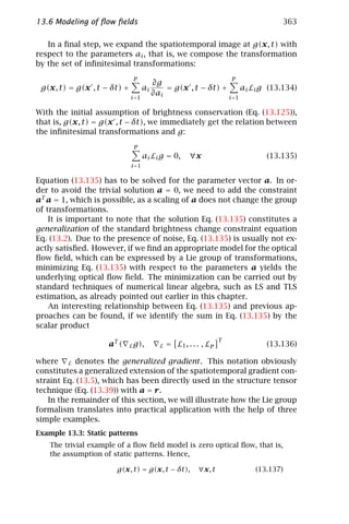
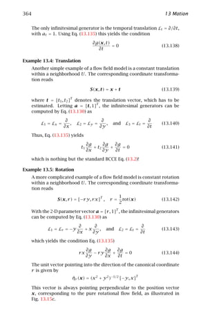
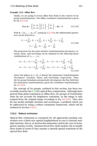
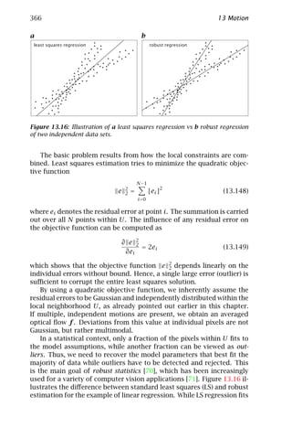
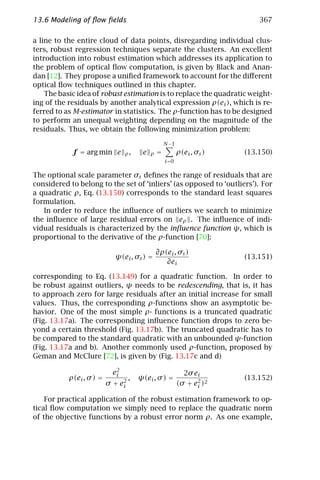
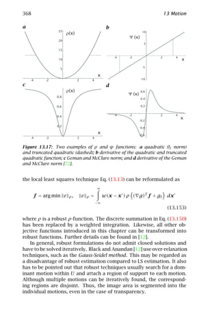
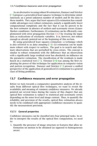
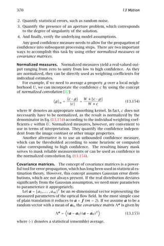
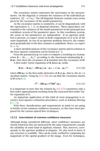
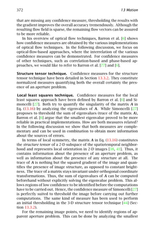
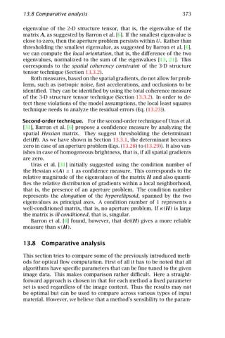
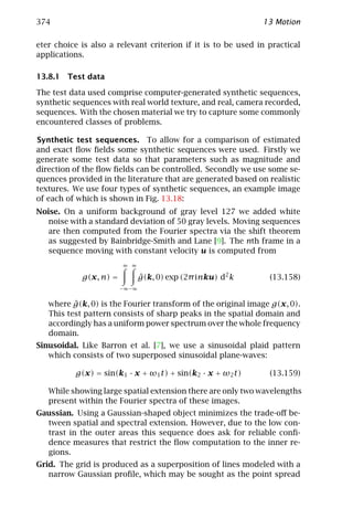
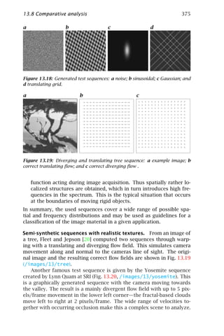
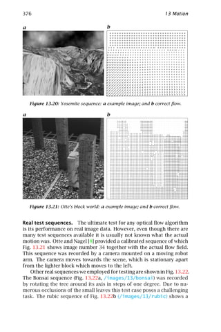
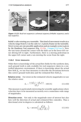
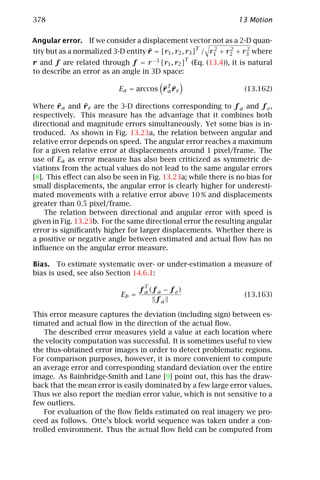
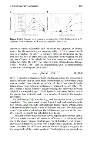
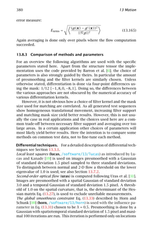
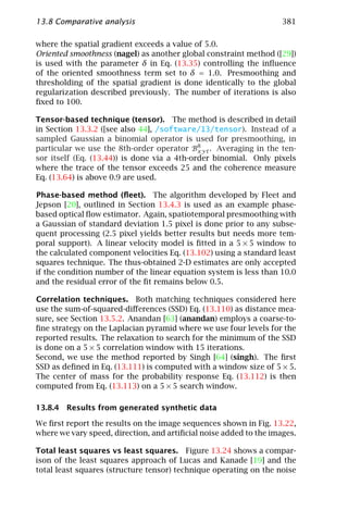
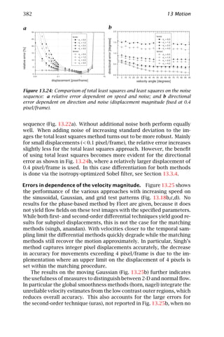
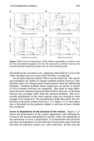
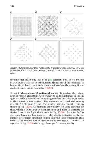
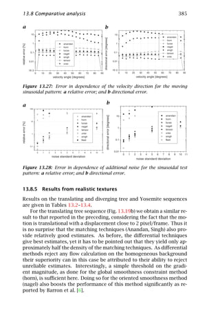
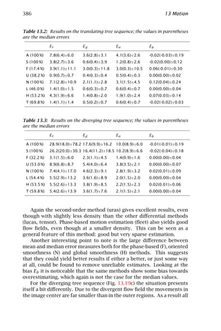
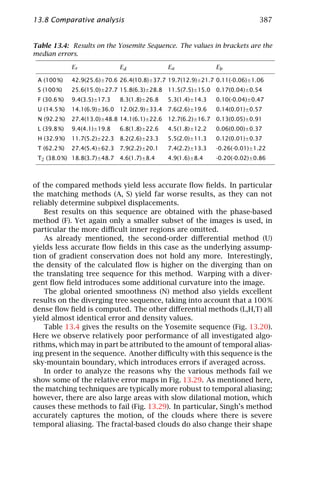
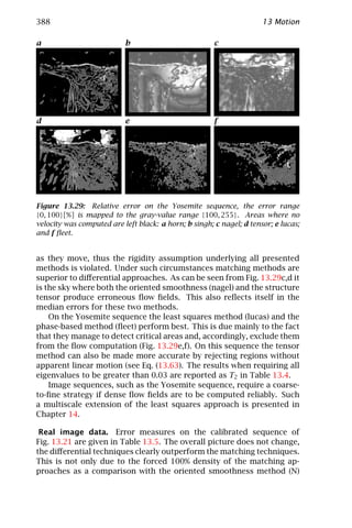
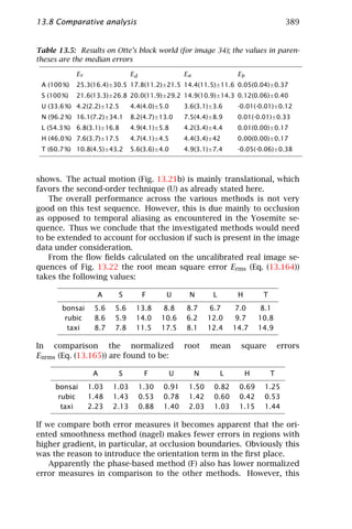
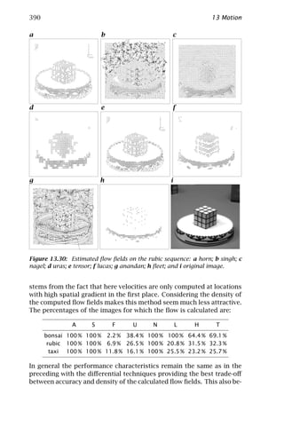
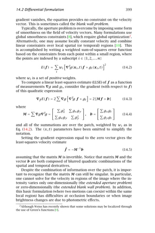
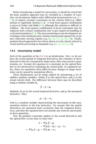
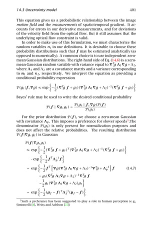

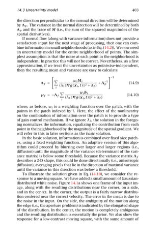
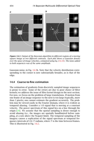
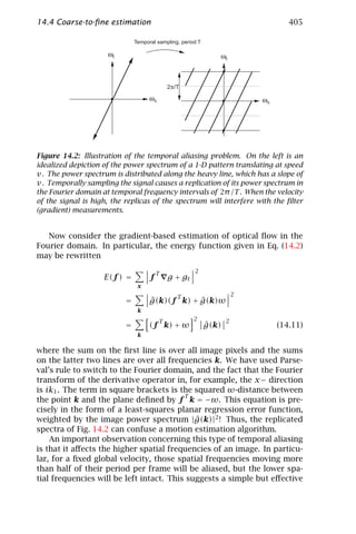
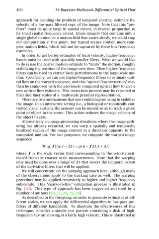
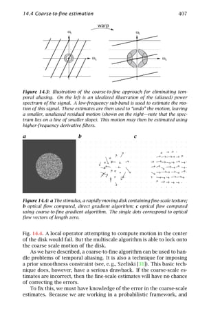
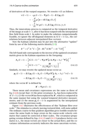
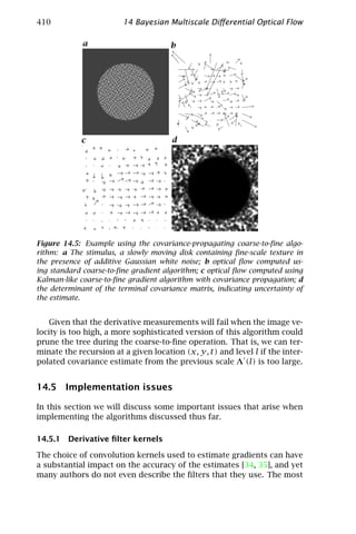
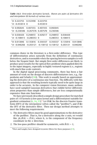
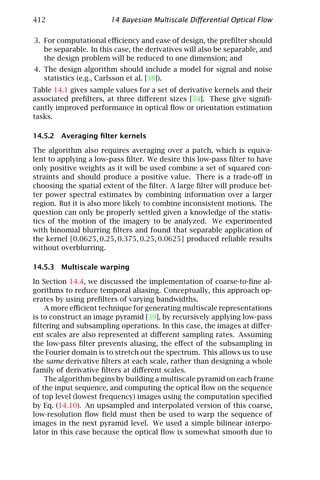
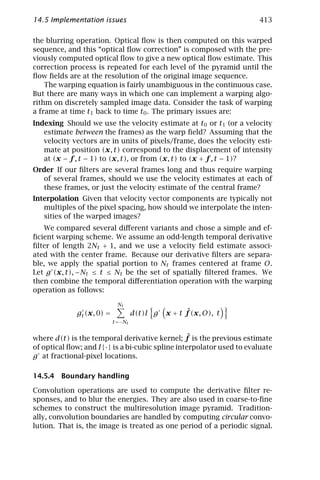
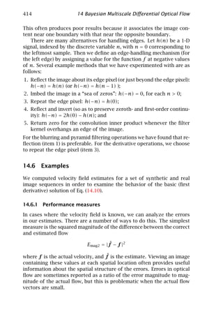
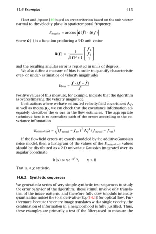
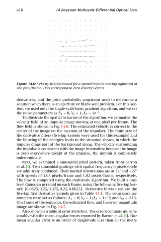
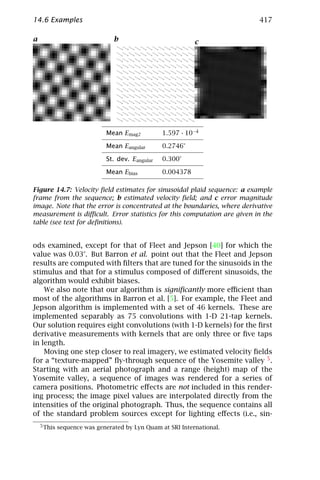
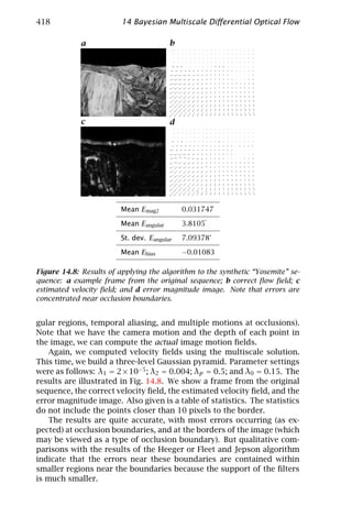
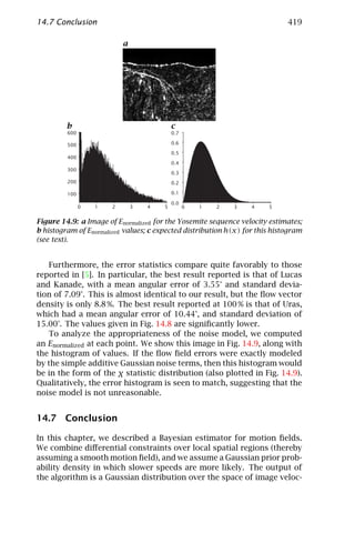
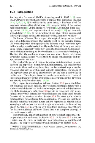
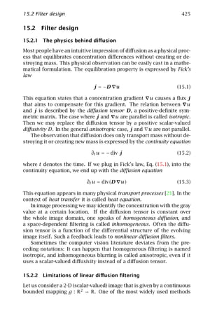
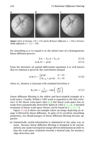
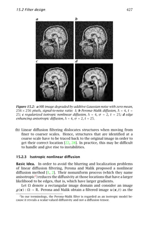
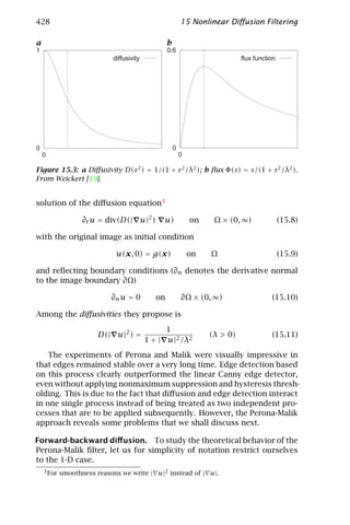
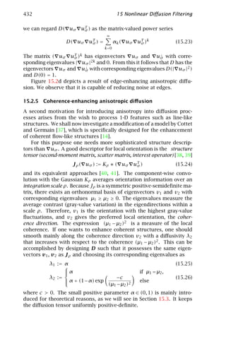
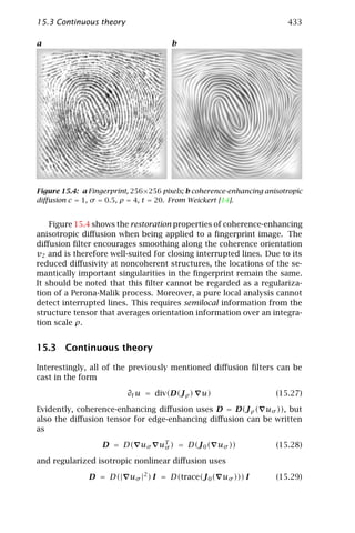
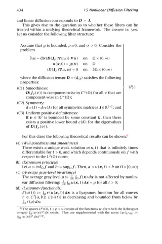
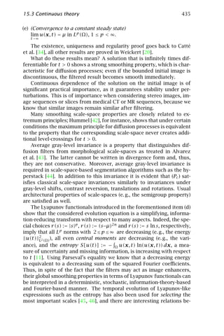
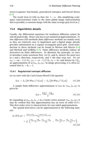
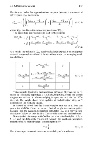
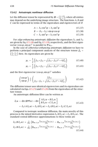
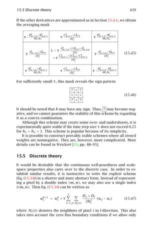
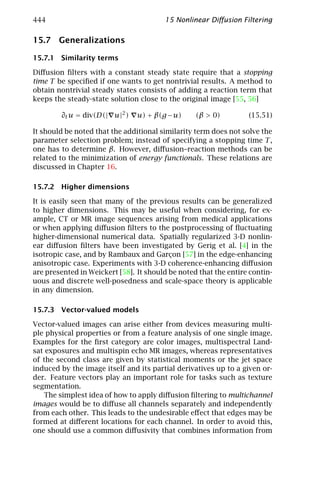
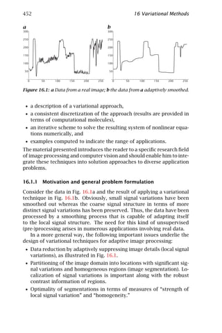
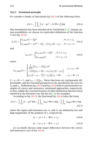
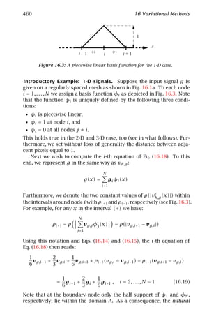
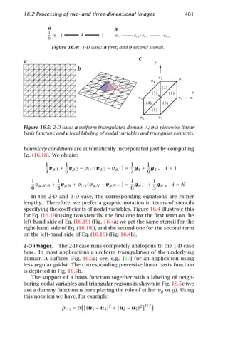
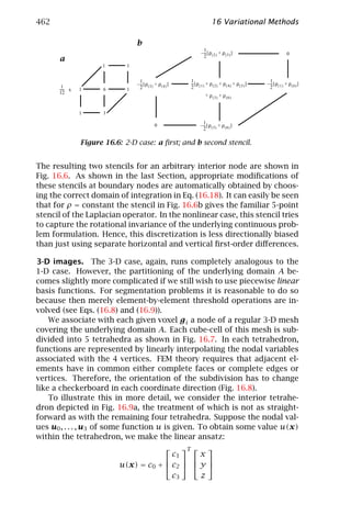
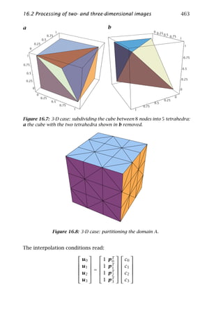
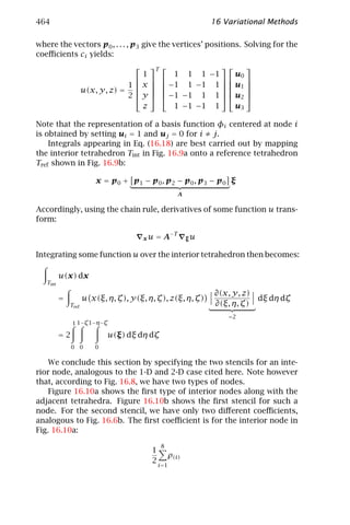
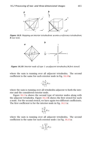
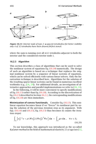
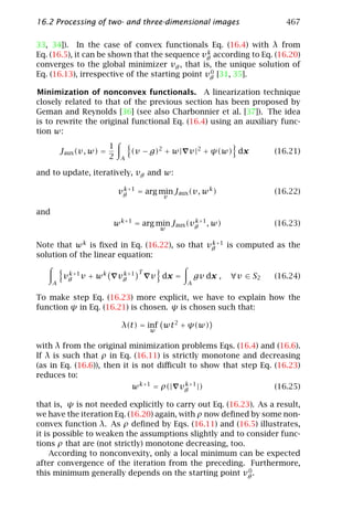
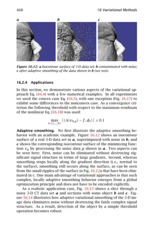
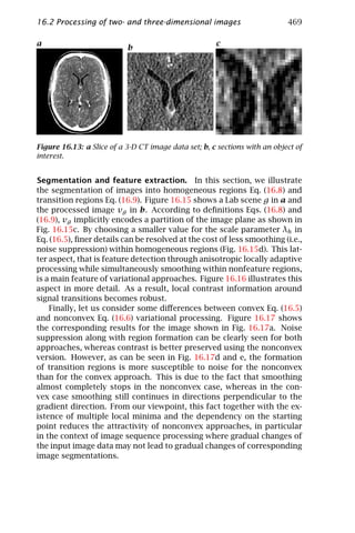
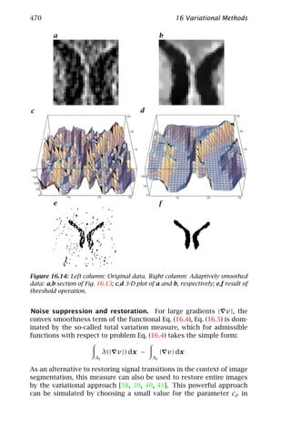
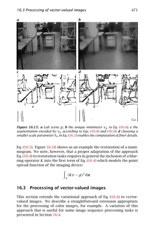
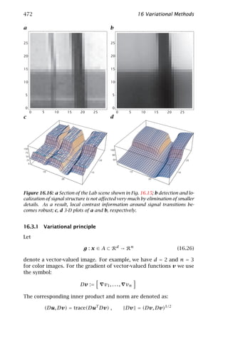
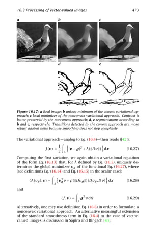
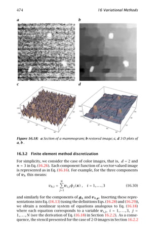
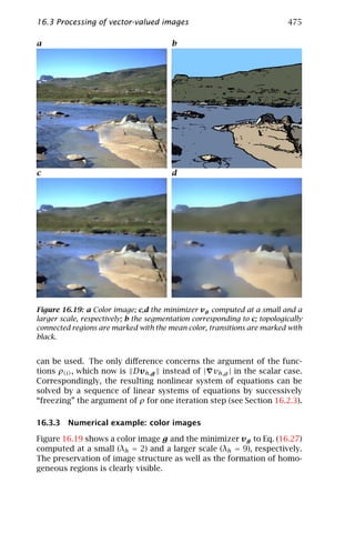
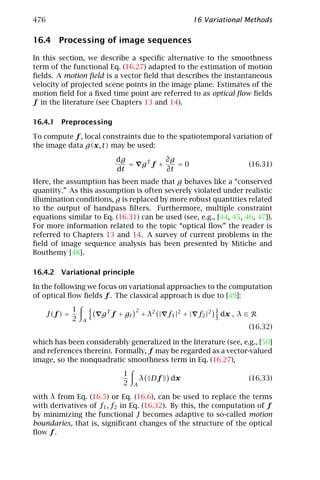
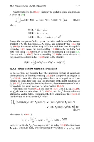
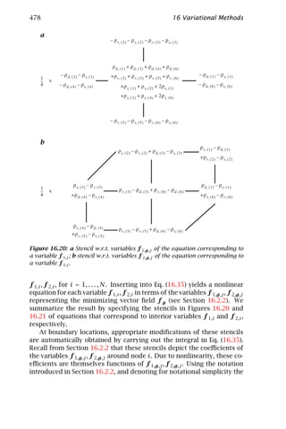
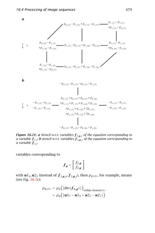
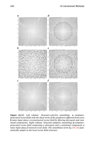
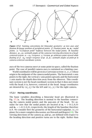
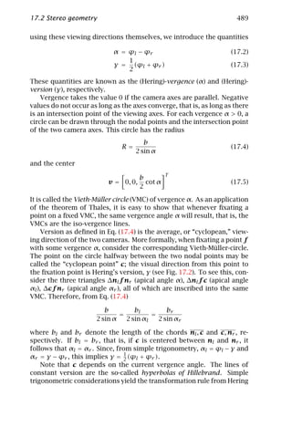
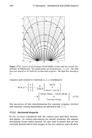
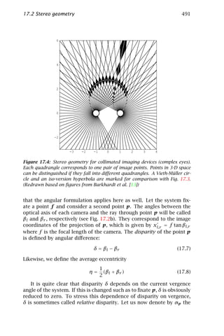
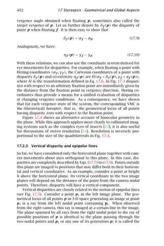
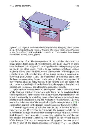
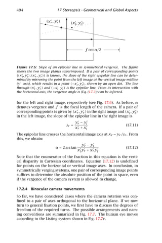
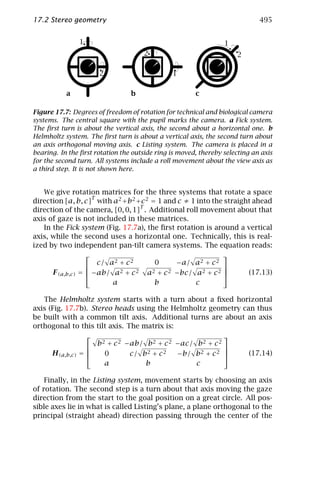
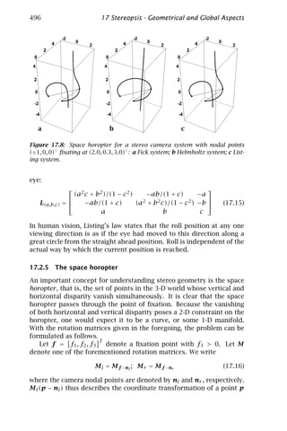
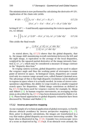
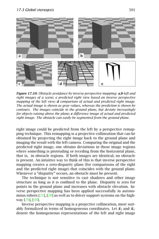
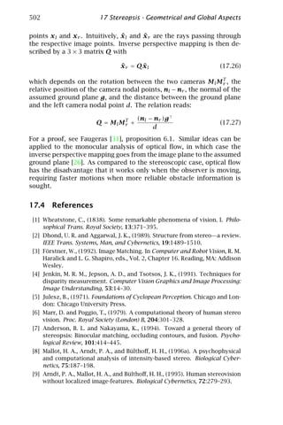
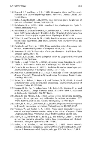
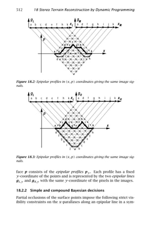
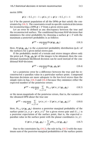
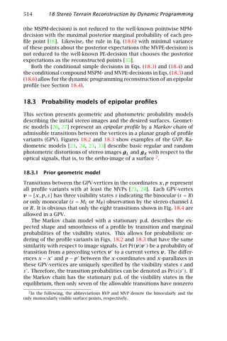
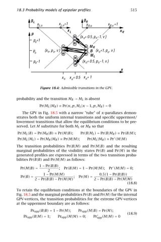
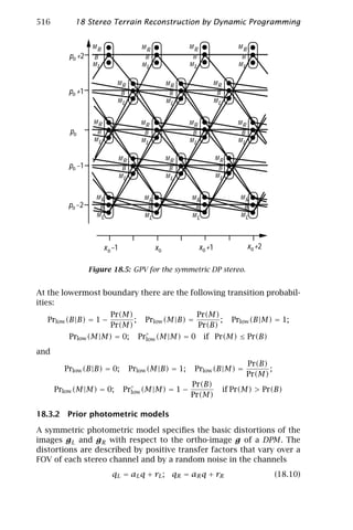
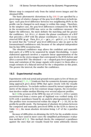
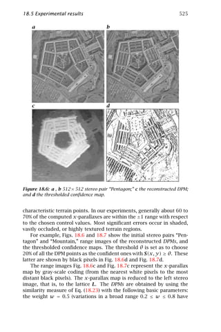
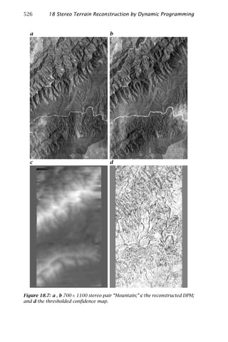
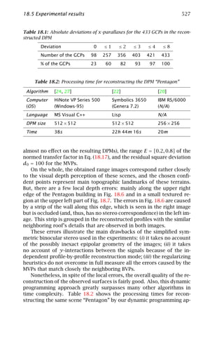
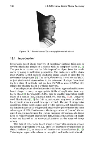
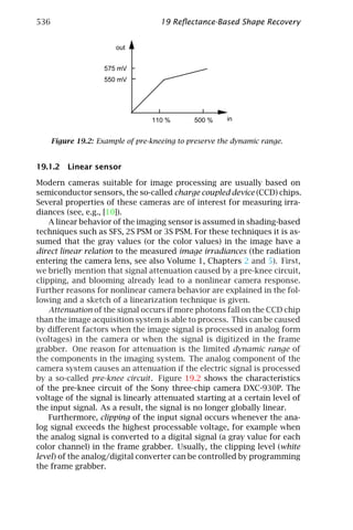
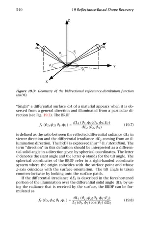
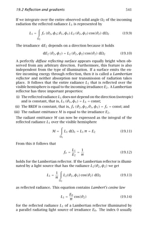
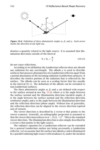
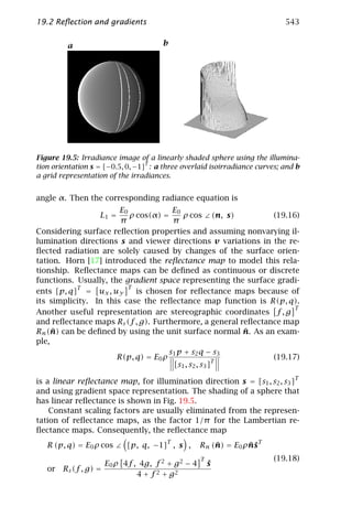
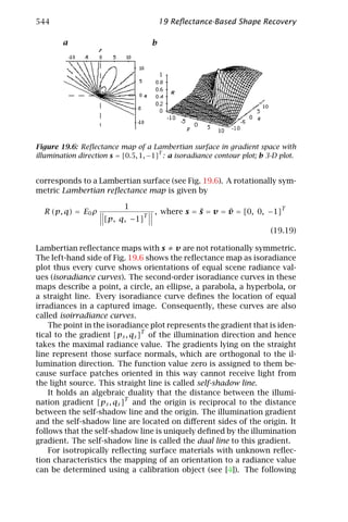
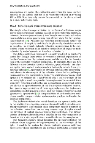
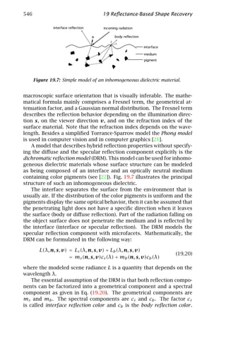
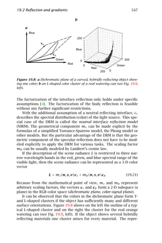
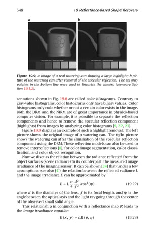
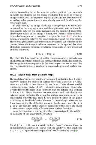
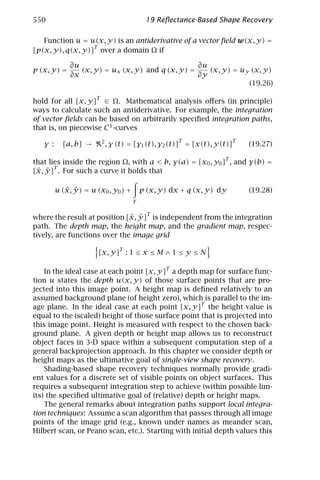
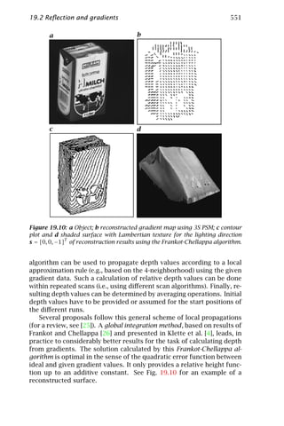
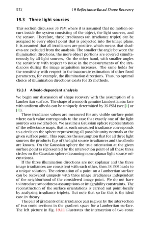
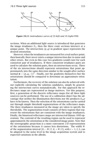
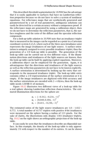
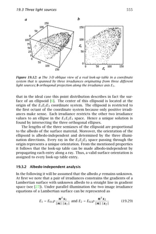
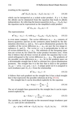
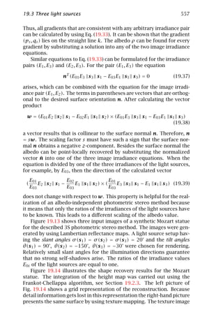
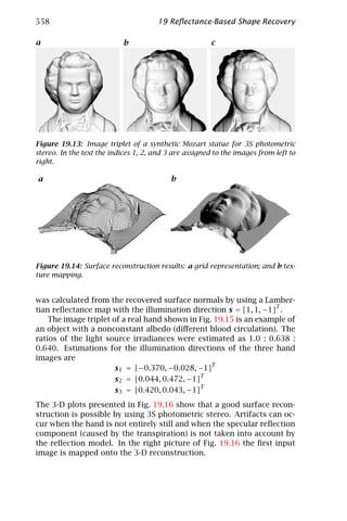
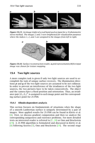
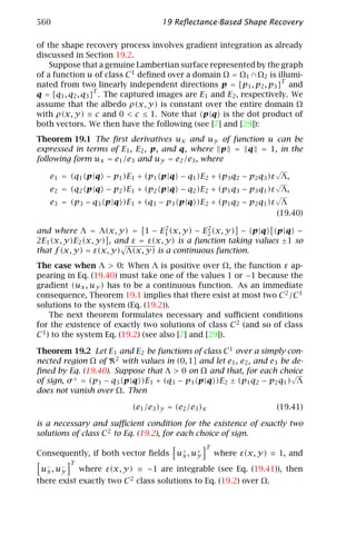
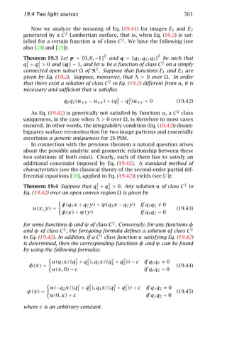
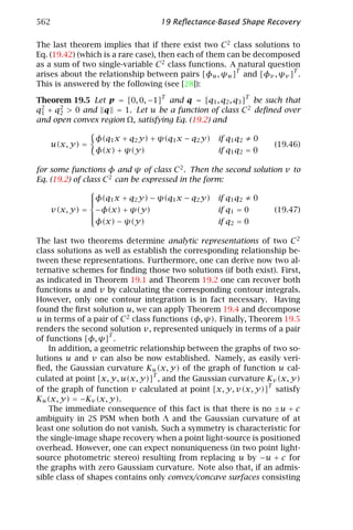
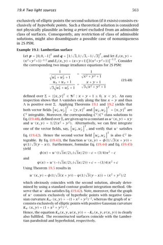
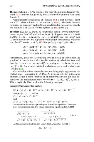
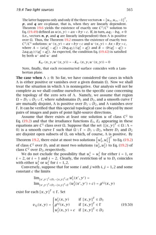
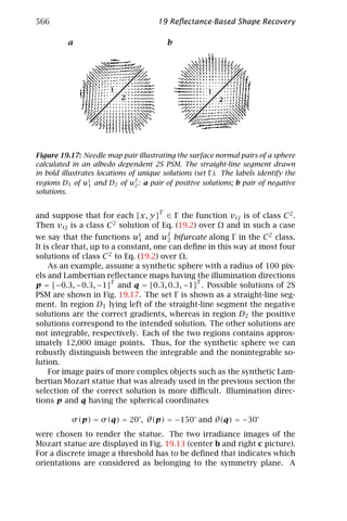
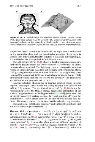
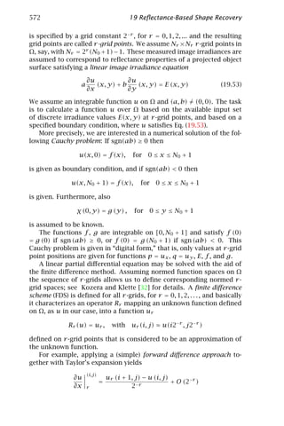
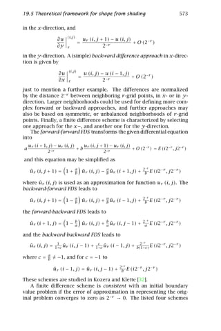
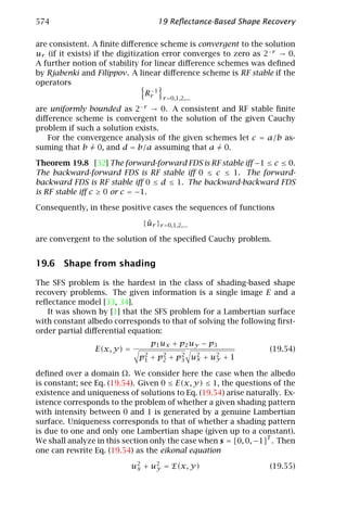
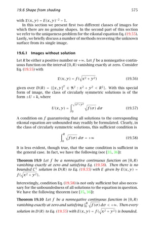
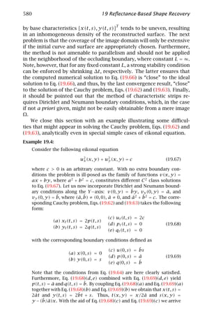
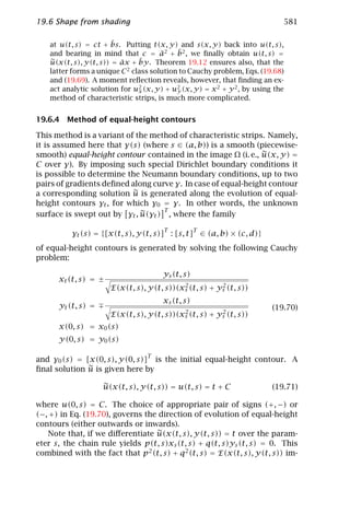
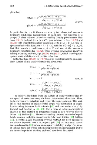
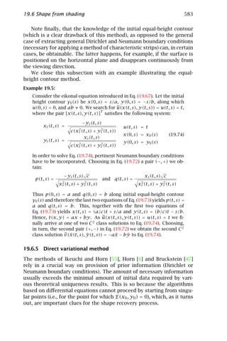
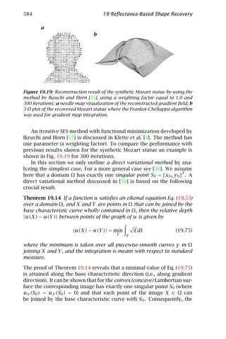
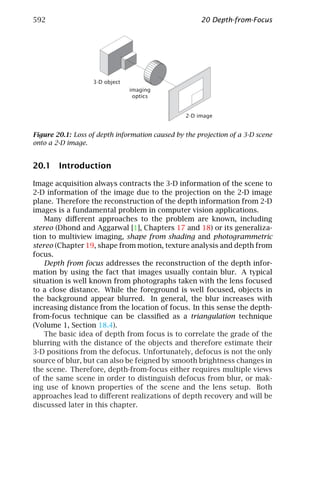
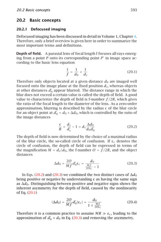
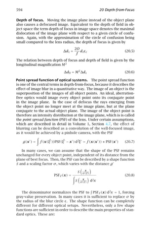
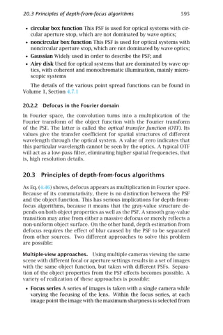
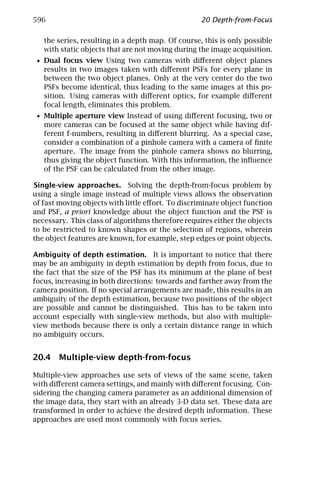
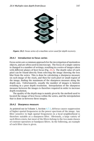
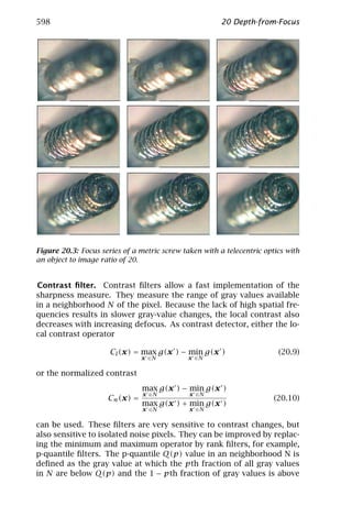
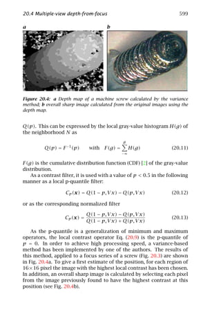
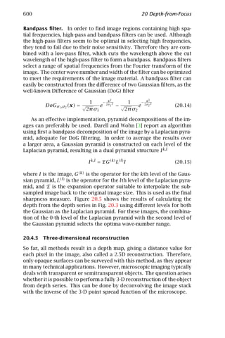
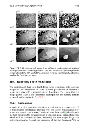
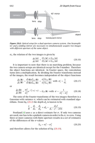
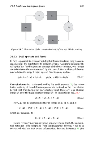
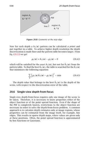
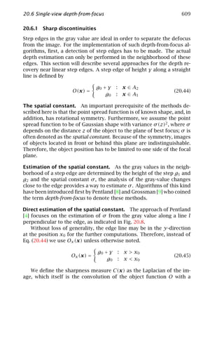
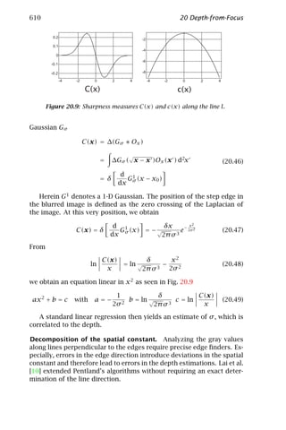
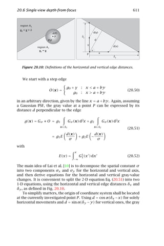
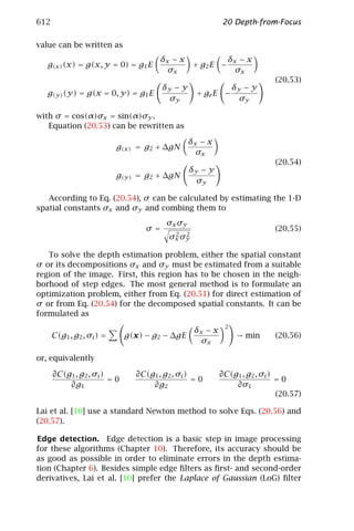
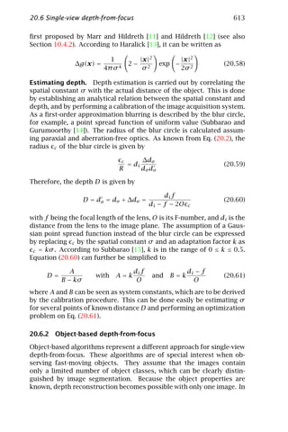
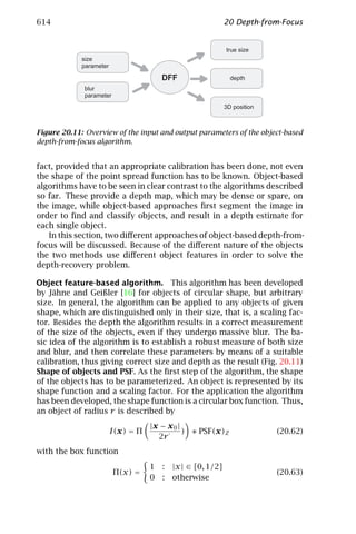
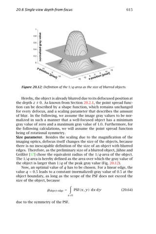
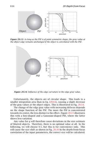
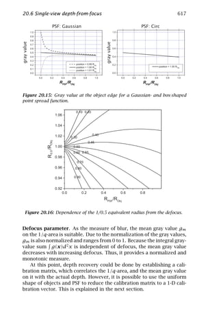
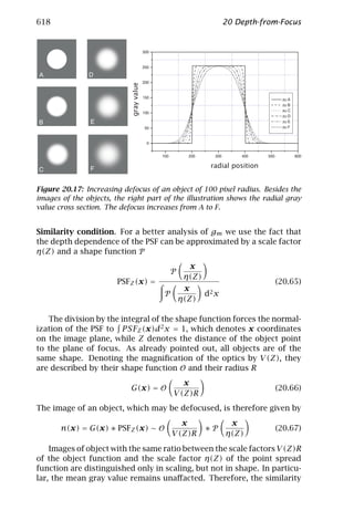
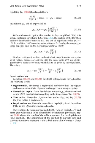
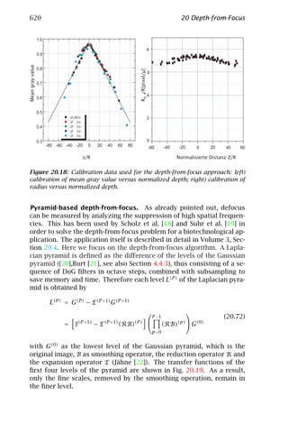
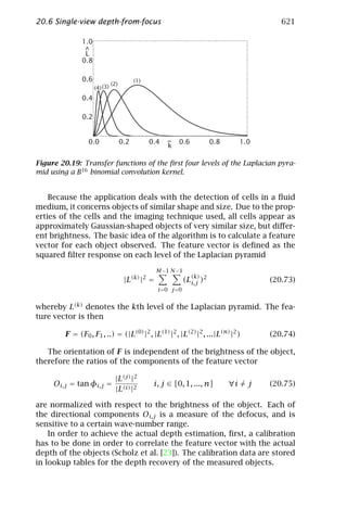


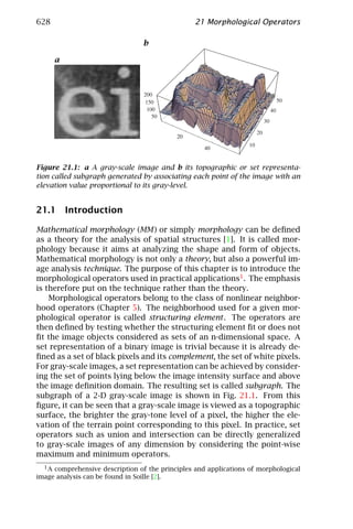
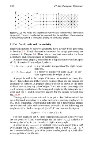
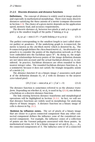
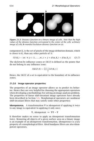
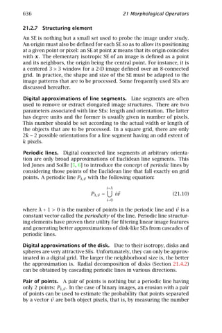
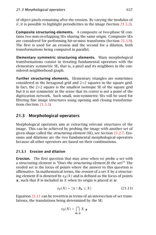
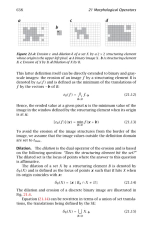
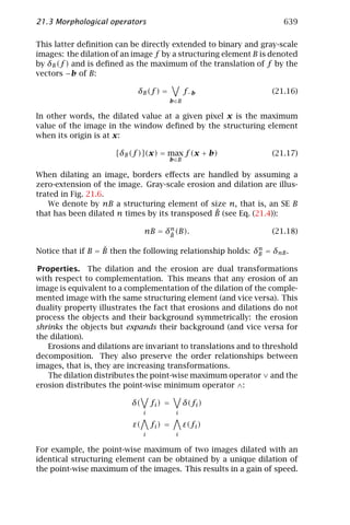
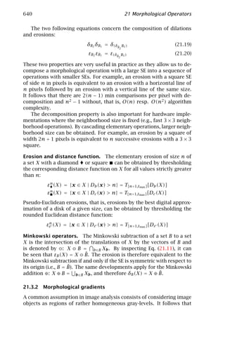
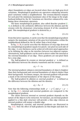
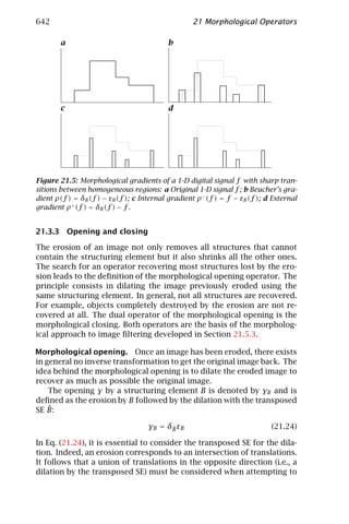
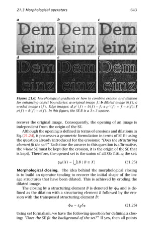
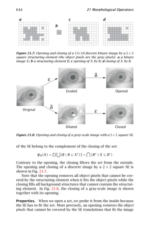
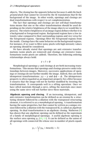
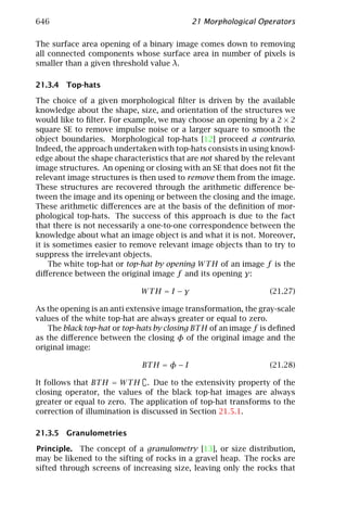
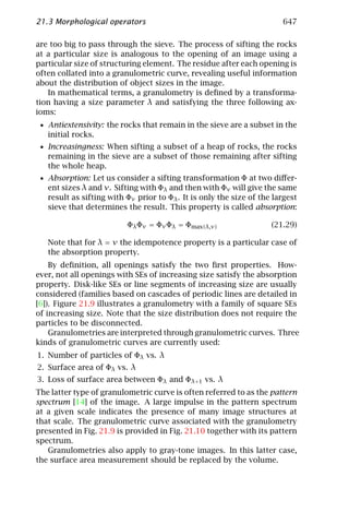
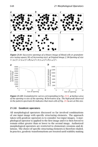
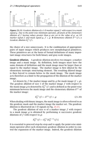
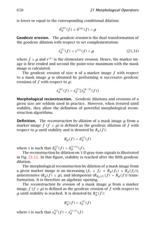
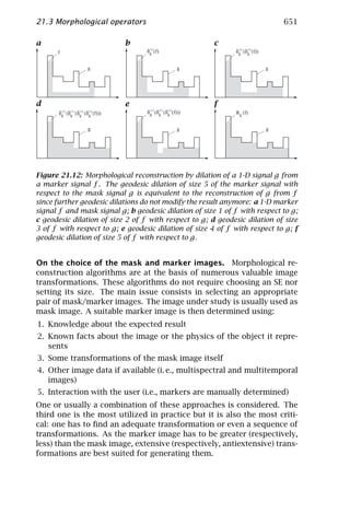
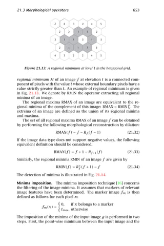
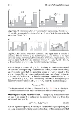
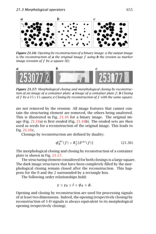
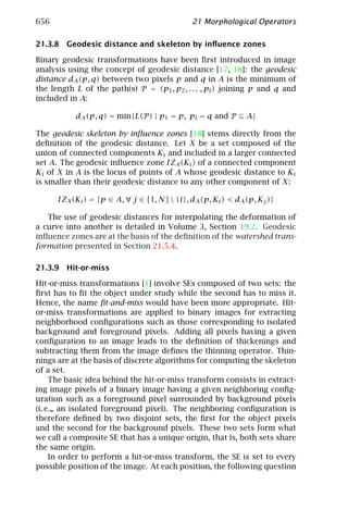
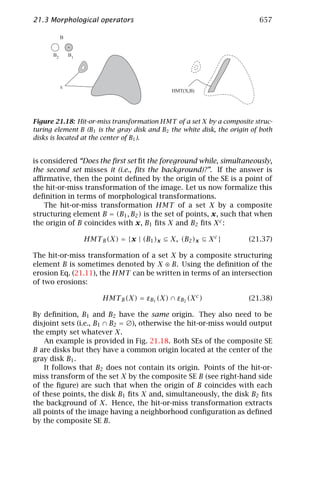
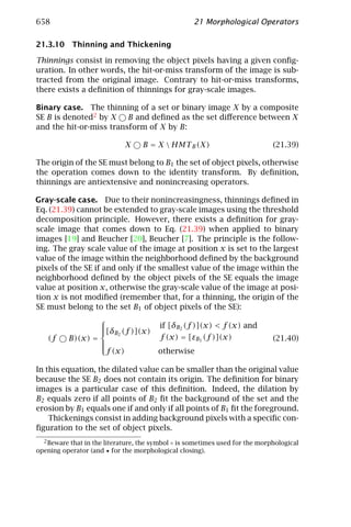
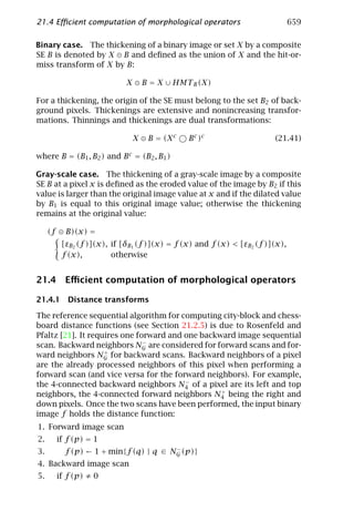
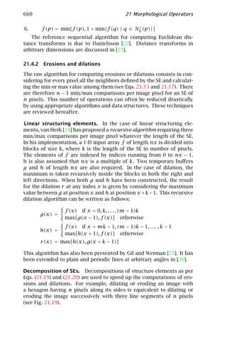
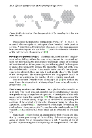
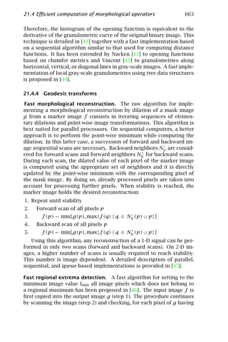
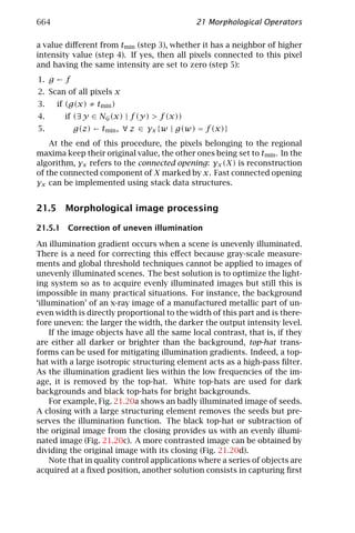
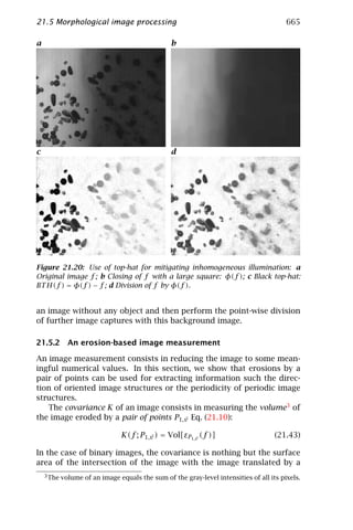
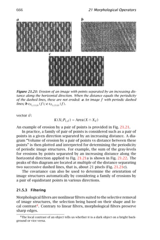
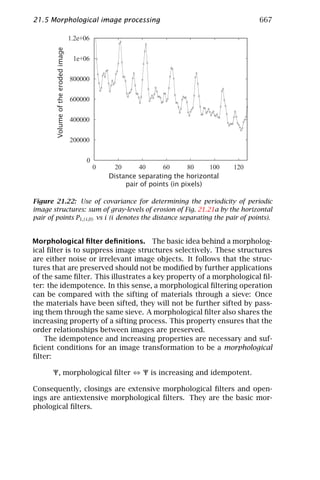
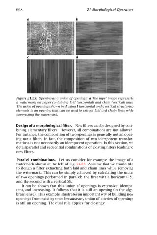
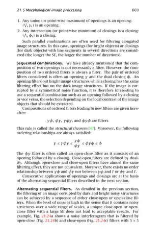
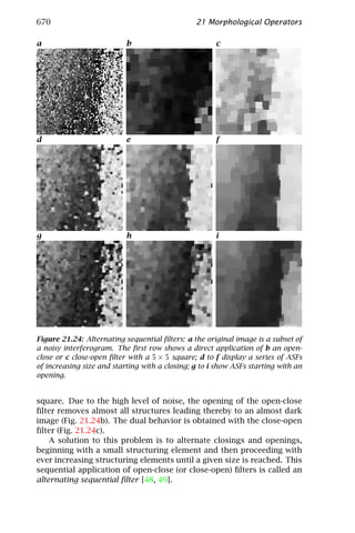
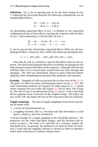
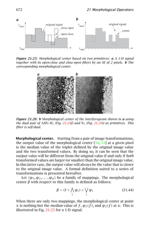
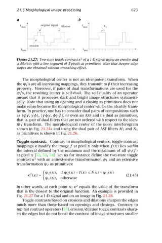
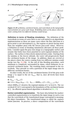
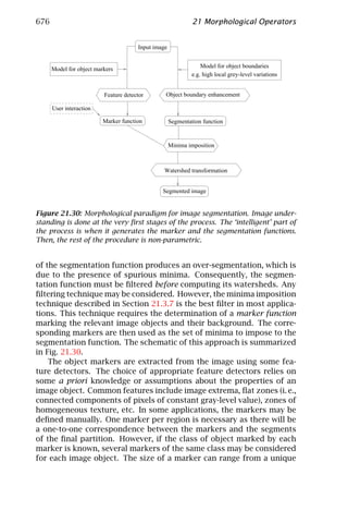

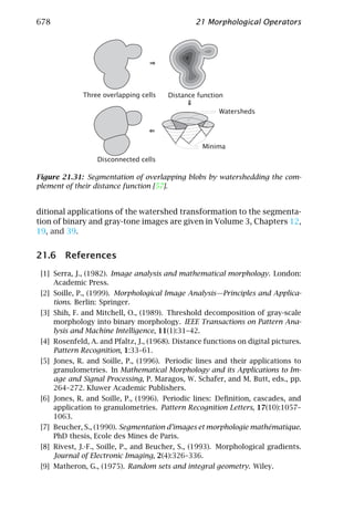

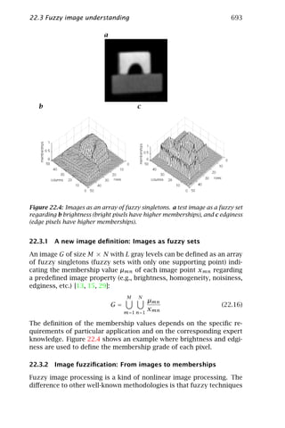
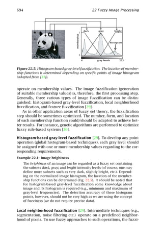
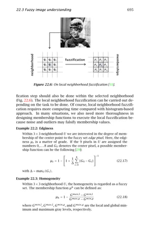
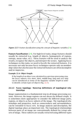
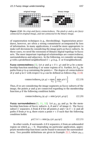
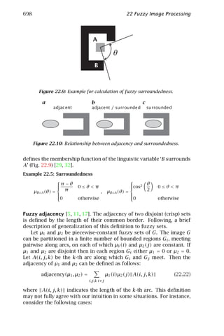
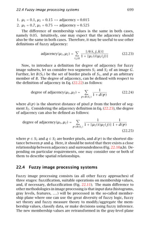
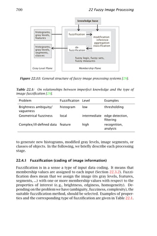
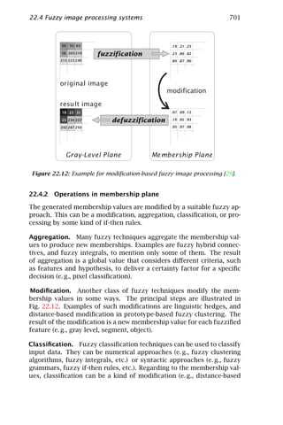
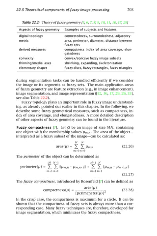
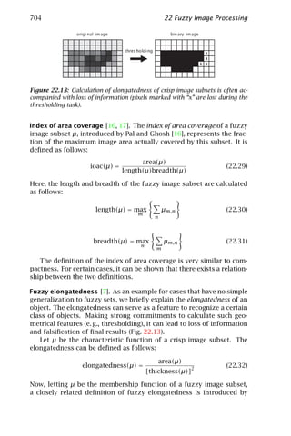
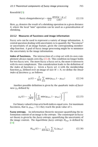
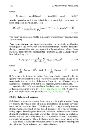
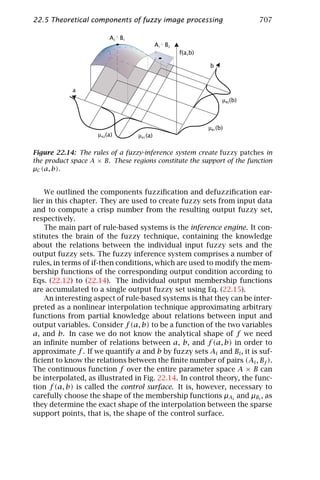
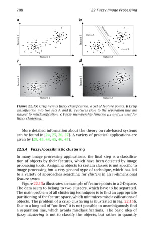
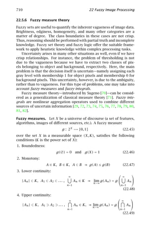
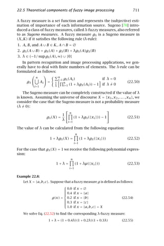
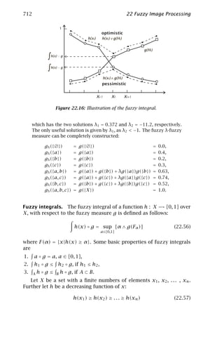
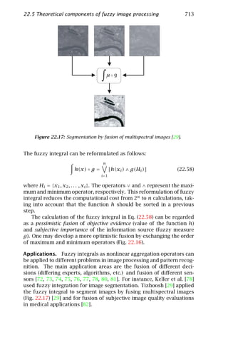
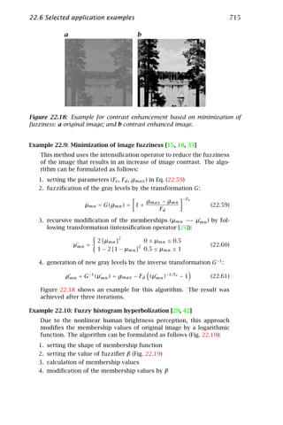
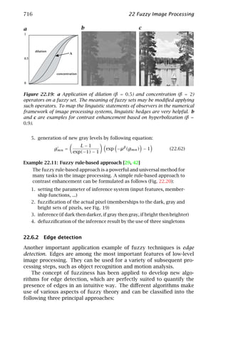
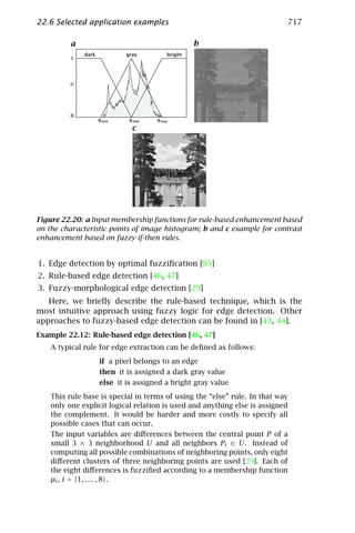
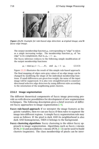
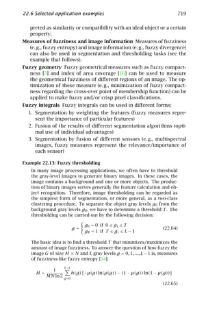
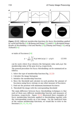
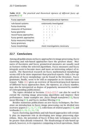

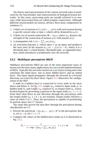
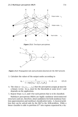
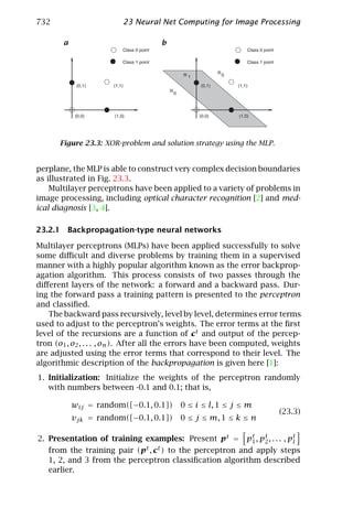
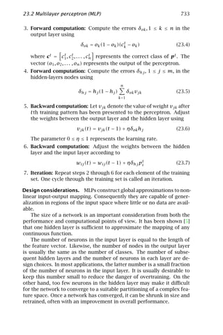
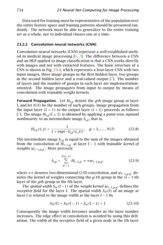
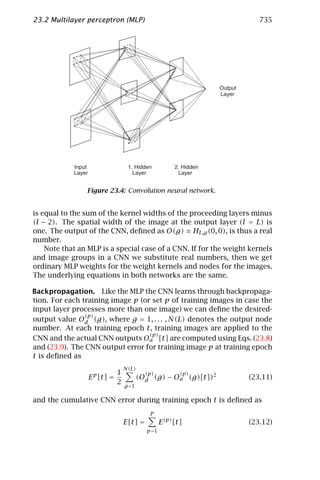
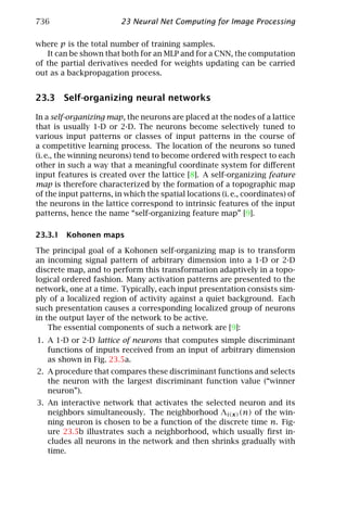
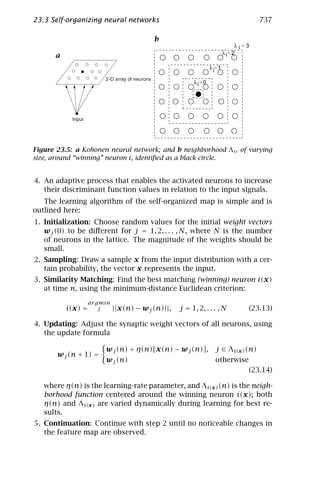
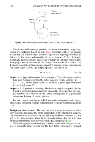
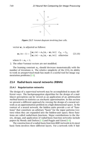
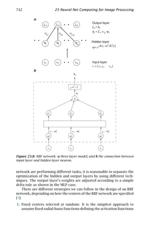
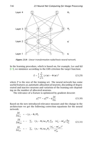
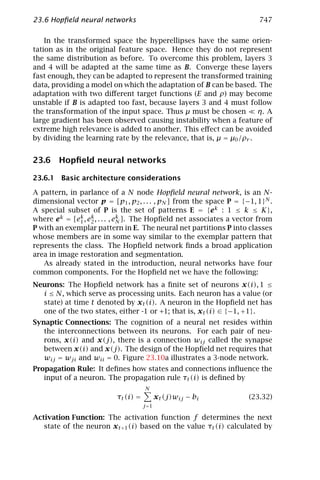
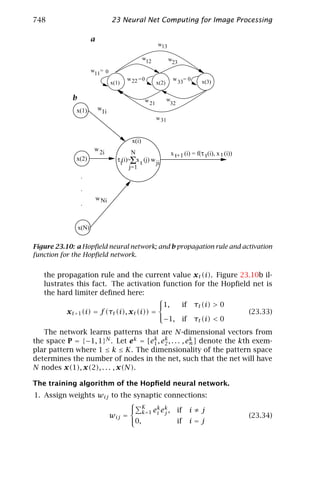
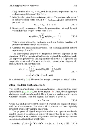
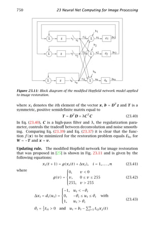
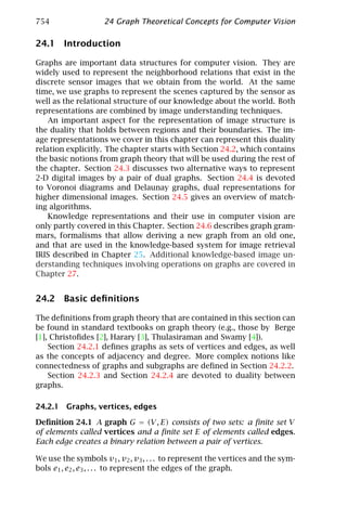
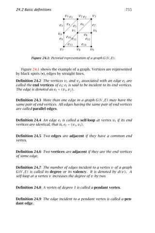
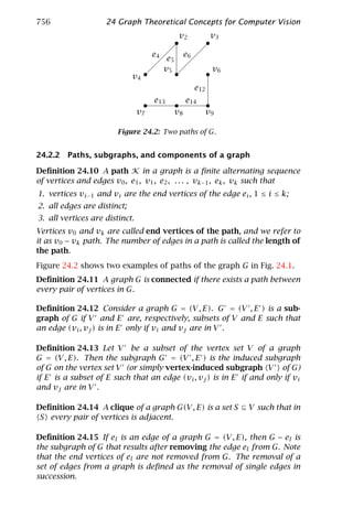
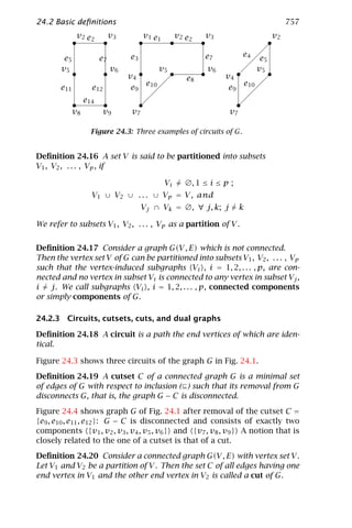
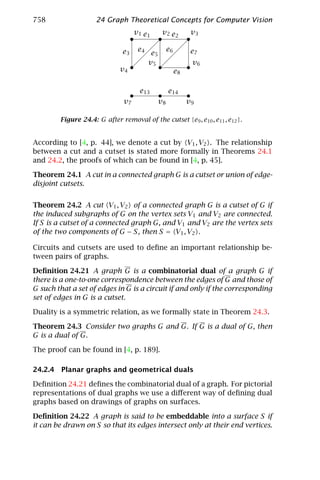
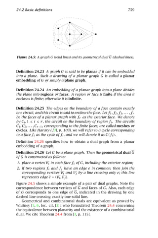
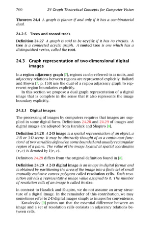
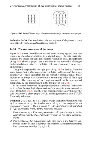
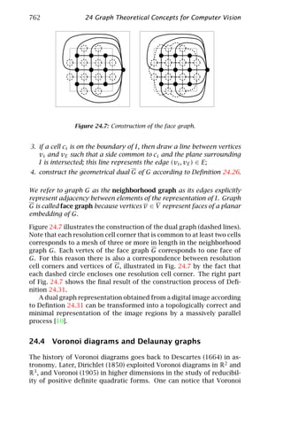
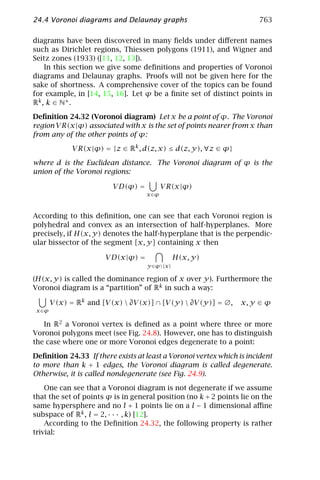
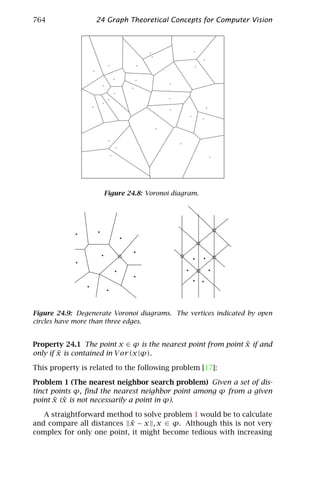
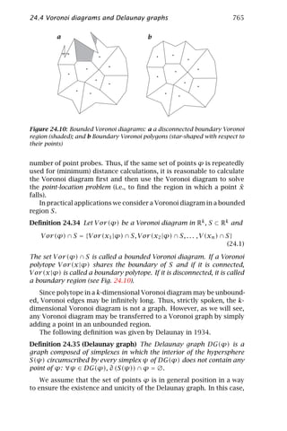
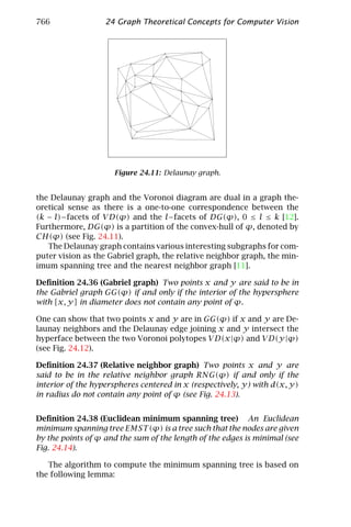
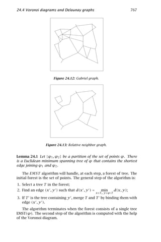
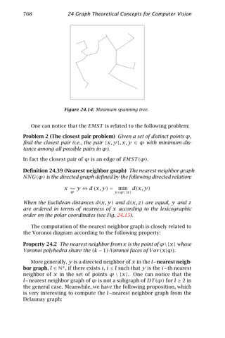
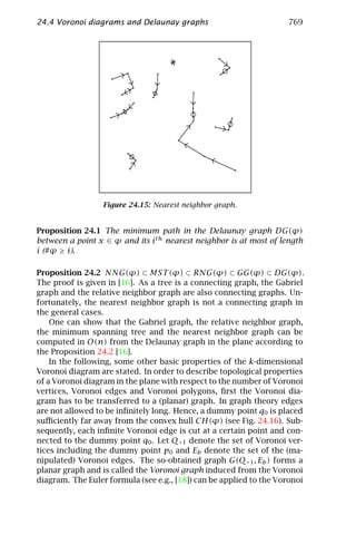
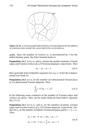
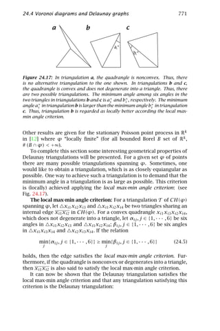
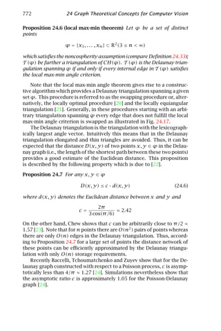
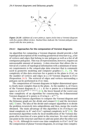
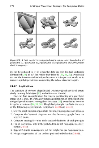
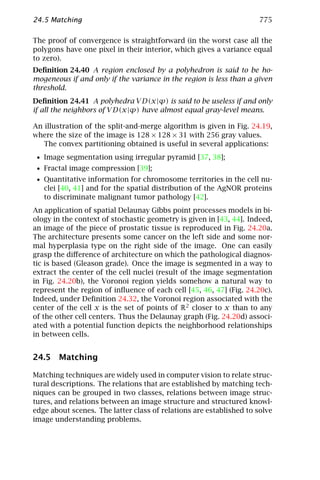
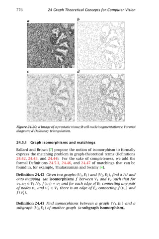
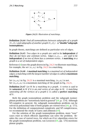
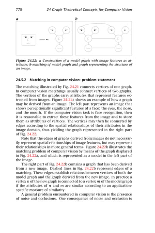
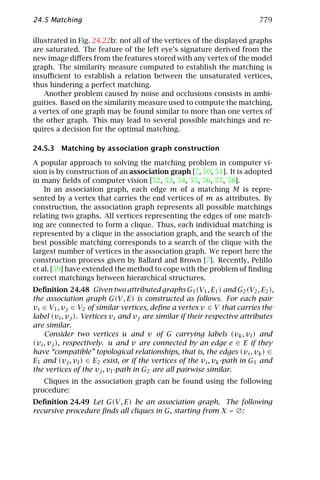
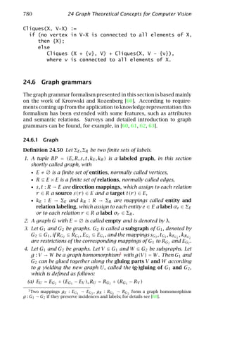
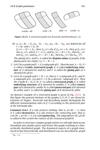
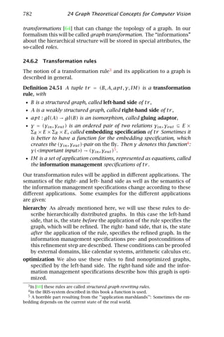
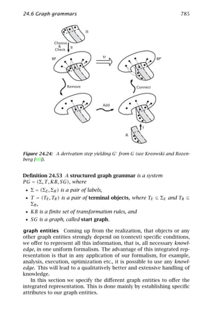
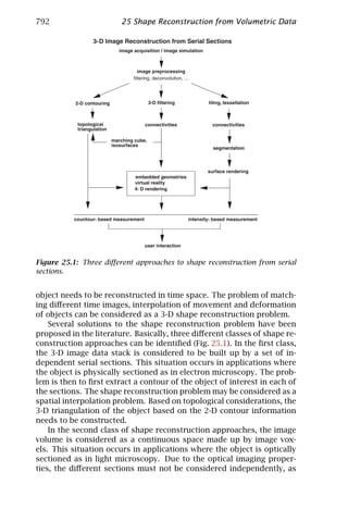
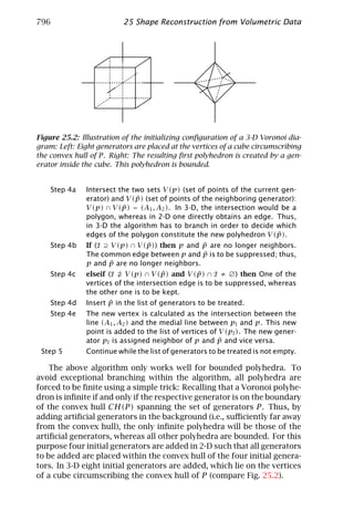
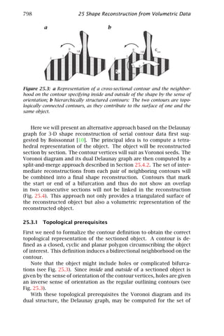
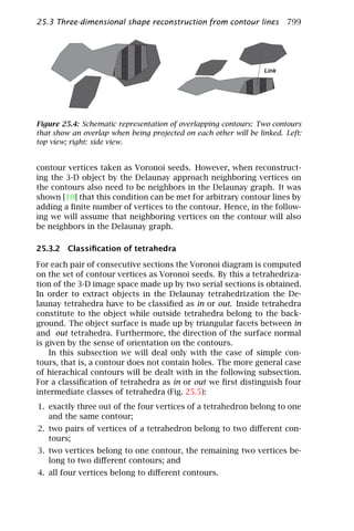
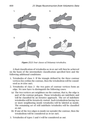
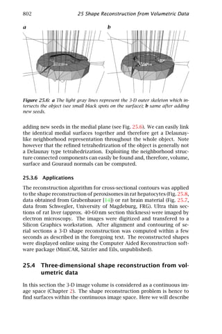
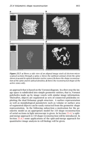
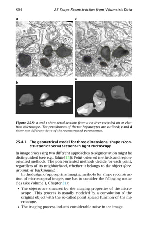
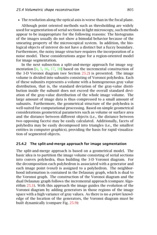
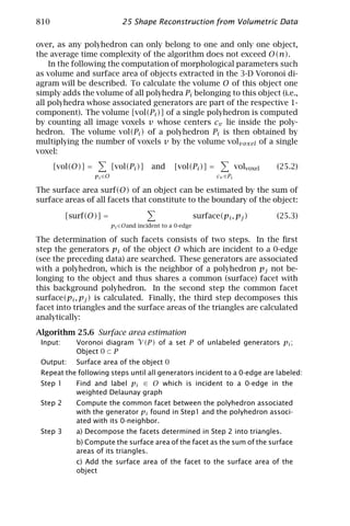
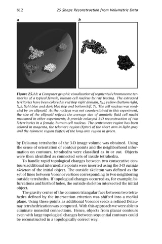


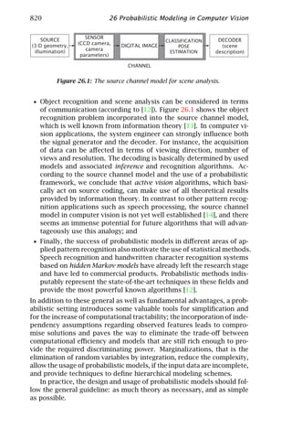
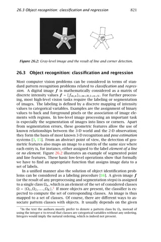

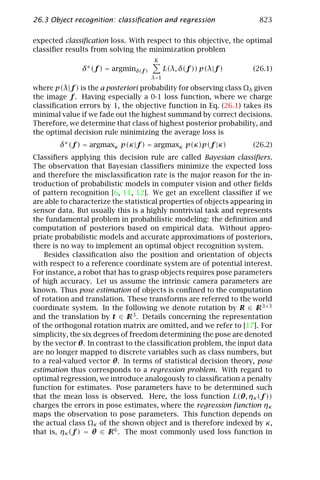
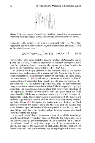
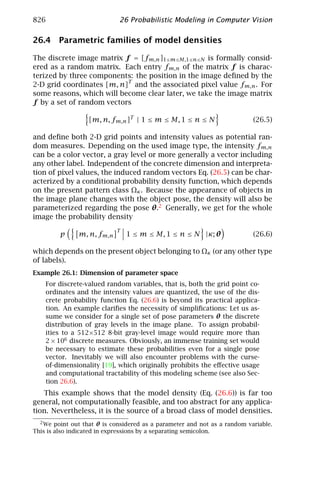
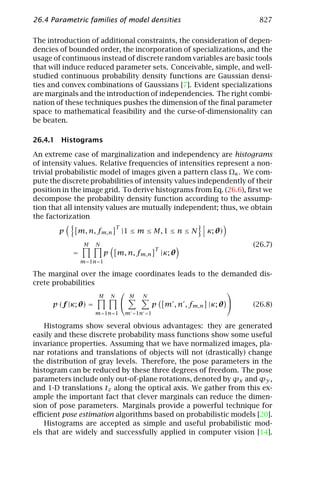
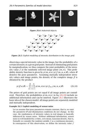
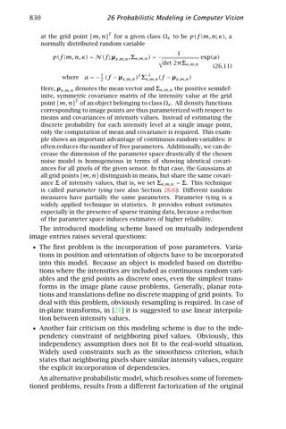
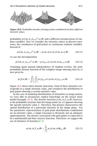
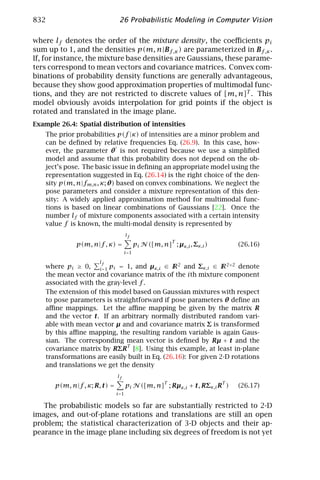
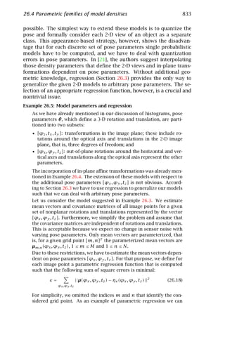
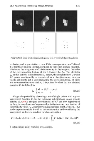
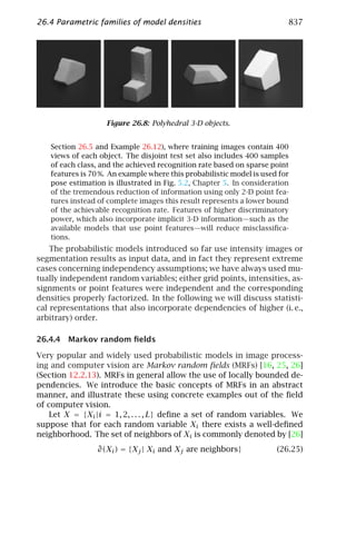
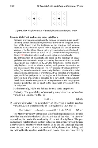
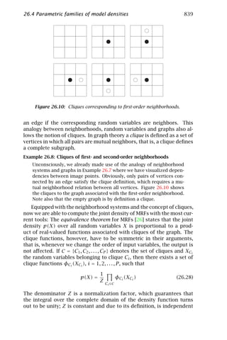
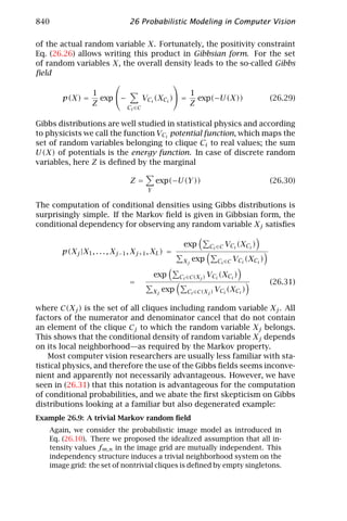
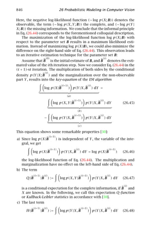
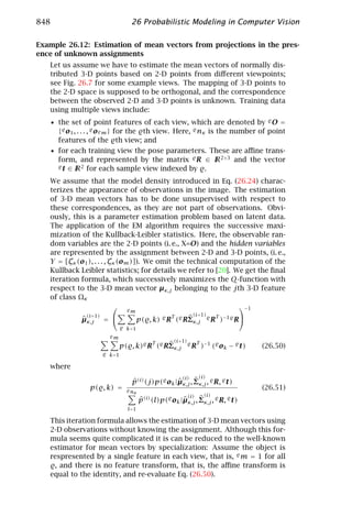
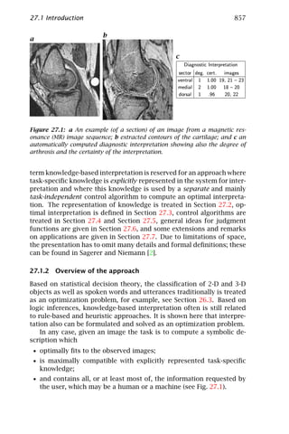
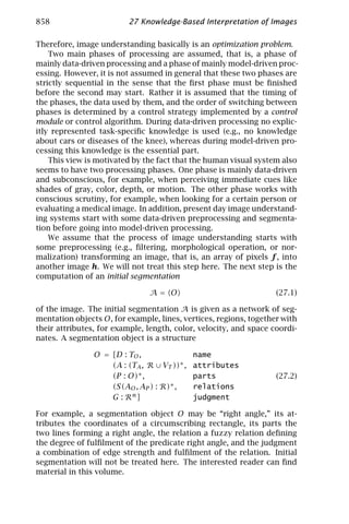
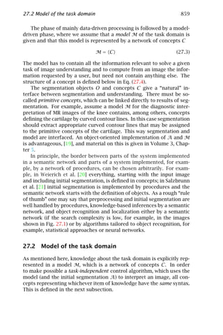
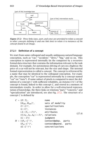
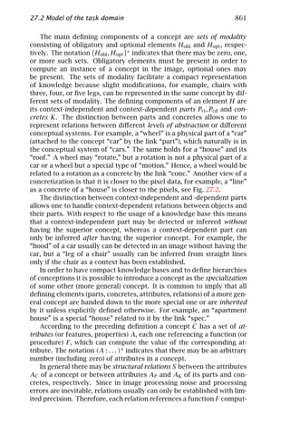
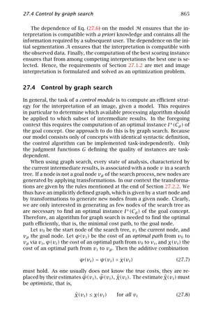
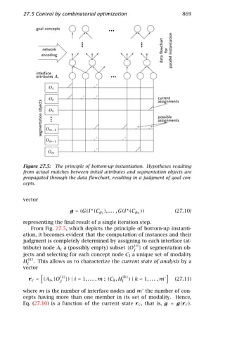
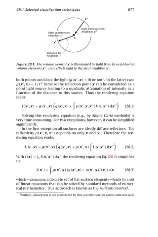
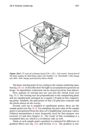
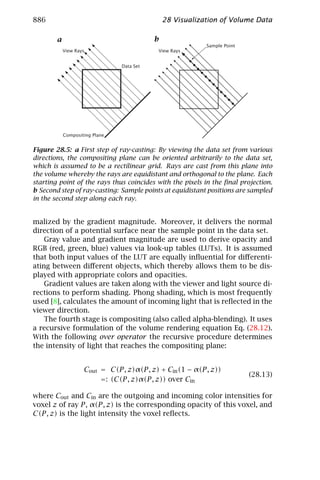
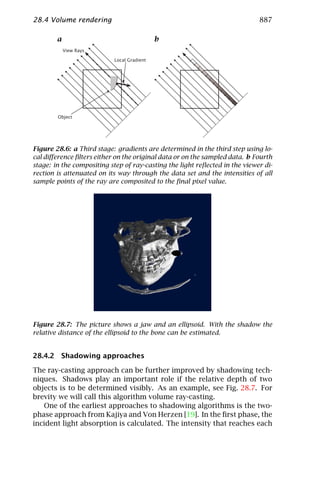
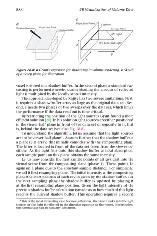
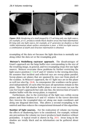
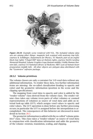
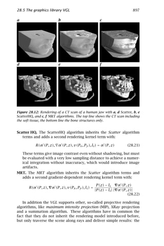
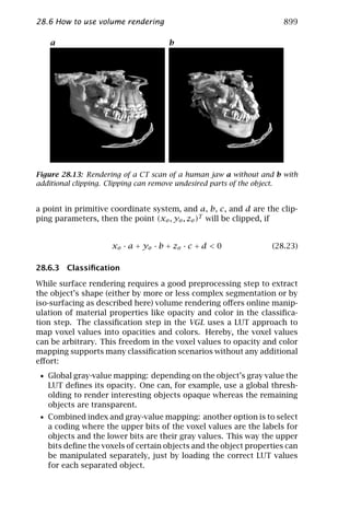
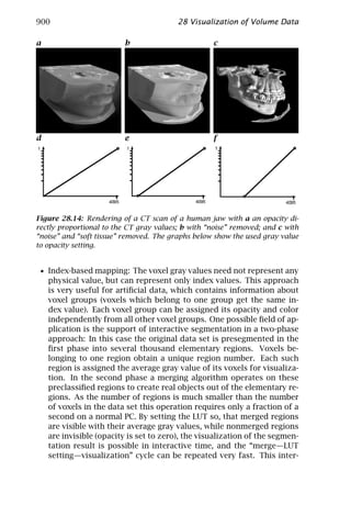
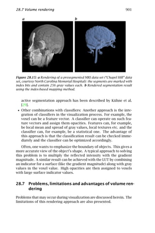
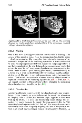
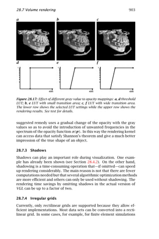
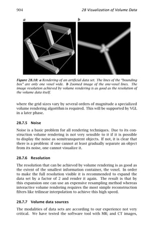
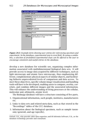

This document provides a summary of a chapter from the book "Handbook of Computer Vision and Applications Volume 2: Signal Processing and Pattern Recognition". The chapter discusses signal processing and pattern recognition techniques that are important for computer vision applications. It covers topics such as signal representation, neighborhood operators, filter design, local averaging, interpolation, and image warping. The document is an introduction to these fundamental computer vision and image processing concepts.