Downloaded 14 times


![4 Chapter 1: Introduction
help to reduce artifacts at the costs of loss of details. Another possibility is interactive correction by
the user which may be helpful if artifacts occur at some few isolated locations.
The opposite of insufficient sampling is that the sample data are unnecessarily dense. This happens
in particular if a surface is sampled with uniform density. In that case the sample density required
at fine details of the surface causes too many data points in regions of only minor variation. Several
approaches to data reduction were proposed in literature [HDD+ 93]. We do not treat this topic here,
but only give the hint that data reduction should consider the power of the reconstruction algorithm
expressed in sampling theorems, a fact that also was not explicitly obeyed in the past.
The challenge of surface reconstruction is to find methods of reconstruction which cover a wide range
of shapes, or, for a given area of application, to find a method of reconstruction which covers the shapes
of this class reasonably. The challenge of data analysis is to find efficient enumeration algorithms
yielding those of all feasible surfaces that come closest to the desired one. In particular, ways must be
found to express which of the possible solutions are favorable.
The wide range of applications from which the data may emerge implies that the data can have quite
different properties which may be considered at the solution of the surface interpolation problem. For
example, the data may be sampled from surfaces that lie unique over a plane. In that case, a wide
range of methods were developed which mainly focus on geometric properties like smoothness of the
constructed surface [HL93].
Reconstruction may become more specific if the surface is captured in multiple samples (multiple
view range images) that have to be fused. Sample fusing may need data transformation and fitting. We
exclude these aspects from further discussion and refer e.g. to [TL94, CL96, SF97].
Sample data may contain additional information on structure. A typical example are tomographic
data. In that case the points on a slice may be already connected by polygonal contour chains. Another
example is that normal vectors are available at the data points. These additional informations may give
additional hints on the unknown surface which may be considered in the construction algorithm. In
particular, for interpolation or approximation of contour data, a variety of methods were developed
[MK93]. In the following, no additional structural information is expected.
Finally, the mathematical and data structural representation of the derived surface has to be consid-
ered. The most common representation is the polygonal or triangular mesh representation. Because
the representation by triangular meshes allows to express the topological properties of the surface, and
because this is the most difficult sub-problem of surface construction, most known algorithms use this
sort of representation. If higher smoothness than just continuity is required, either the parametric or the
implicit surface representation may be used. Triangular meshes can be seen as a surface composed by
parametrically represented linear surface patches. For surfaces of higher continuity patches of higher
order are required. One way to obtain such surfaces is to start from a triangular mesh. For that reason,
we have chosen the representation by triangular meshes for this thesis, and refer to literature for the
problem of deriving smooth surfaces, for instance to [EH96, Guo97, FCGA97] in which smoothing of
surfaces obtained from sample data is particularly emphasized.
1.2 The Contributions
In this thesis, a new surface reconstruction algorithm is presented which works well in practice, as has
been demonstrated by application of an implementation to numerous data sets. Its particular features
are
(1) reconstruction of open surfaces with boundaries of arbitrary genus as well as non-orientable
surfaces,](https://image.slidesharecdn.com/surfacereconstructionrobertmenclphdthesis-130112202114-phpapp01/85/Reconstruction-of-Surfaces-from-Three-Dimensional-Unorganized-Point-Sets-Robert-Mencl-PhD-Thesis-12-320.jpg)

![Chapter 2
State of the Art
The surface construction problem has found considerable interest in the past, and is still an important
topic of research. The purpose of this chapter is to find unifying basic methods common to indepen-
dently developed solutions, coupled with a survey of existing algorithms. The identified basic classes
are constructions based on spatial subdivision (Section 2.1), on distance functions (Section 2.2), on
warping (Section 2.3), and on incremental surface growing (Section 2.4). In Section 2.5 the aspect is
treated that an object represented in a sample data set may consist of several connected components.
The survey closes with a discussion and categorization of our approach (Section 2.6).
2.1 Spatial Subdivision
Common to the approaches that can be characterized by ”spatial subdivision” is that a bounding box of
the set P of sample points is subdivided into disjoint cells. There is a variety of spatial decomposition
techniques which were developed for different applications [LC87]. Typical examples are regular
grids, adaptive schemes like octrees, or irregular schemes like tetrahedral meshes. Many of them can
also be applied to surface construction.
The goal of construction algorithms based on spatial subdivision is to find cells related to the shape
described by P . The cells can be selected in roughly two ways: surface–oriented and volume–oriented.
2.1.1 Surface–Oriented Cell Selection
The surface–oriented approach consists of the following basic steps.
Surface–oriented cell selection:
1. Decompose the space in cells.
2. Find those cells that are traversed by the surface.
3. Calculate a surface from the selected cells.
The Approach of Algorri and Schmitt
An example for surface–oriented cell selection is the algorithm of Algorri and Schmitt [AS96]. For
the first step, the rectangular bounding box of the given data set is subdivided by a regular ”voxel
grid”. ”Voxel” stands for ”volume element” and denotes a spatial cell of the grid.
In the second step, the algorithm extracts those voxels which are occupied by at least one point of
the sample set P . In the third step, the outer quadrilaterals of the selected voxels are taken as a first
approximation of the surface. This resembles the cuberille approach of volume visualization [HL79].
7](https://image.slidesharecdn.com/surfacereconstructionrobertmenclphdthesis-130112202114-phpapp01/85/Reconstruction-of-Surfaces-from-Three-Dimensional-Unorganized-Point-Sets-Robert-Mencl-PhD-Thesis-15-320.jpg)
![8 Chapter 2: State of the Art
In order to get a more pleasant representation, the surface is transferred into a triangular mesh by
diagonally splitting each quadrilateral into two triangles. The cuberille artifacts are smoothed using
a low–pass filter that assigns a new position to each vertex of a triangle. This position is computed
as the weighted average of its old position and the position of its neighbors. The approximation of
the resulting surface is improved by warping it towards the data points. For more on that we refer to
Section 2.3.2.
The Approach of Hoppe et al.
Another possibility of surface–oriented cell selection is based on the distance function approach of
Hoppe [HDD+ 92, HDD+ 93, Hop94].
The distance function of the surface of a closed object tells for each point in space its minimum signed
distance to the surface. Points on the surface of course have distance 0, whereas points outside the
surface have positive, and points inside the surface have negative distance. The calculation of the
distance function is outlined in Section 2.2.1.
The first step of the algorithm again is implemented by a regular voxel grid. The voxel cells selected
in the second step are those which have vertices of opposite sign. Evidently, the surface has to traverse
these cells. In the third step, the surface is obtained by the marching cubes algorithm of volume
visualization [LC87]. The marching cubes algorithm defines templates of separating surface patches
for each possible configuration of the signs of the distance values at the vertices of a voxel cell.
The voxels are replaced with these triangulated patches. The resulting triangular mesh separates the
positive and negative distance values on the grid.
A similar algorithm has been suggested by Roth and Wibowoo [RW97]. It differs from the approach
of Hoppe et al. in the way the distance function is calculated, cf. Section 2.2.1. Furthermore, the
special cases of profile lines and multiple view range data are considered besides scattered point data.
A difficulty with these approaches is the choice of the resolution of the voxel grid. One effect is that
gaps may occur in the surface because of troubles of the heuristics of distance function calculation.
The Approach of Bajaj, Bernardini et al.
The approach of Bajaj, Bernardini et al. [BBX95] differs from the previous ones in that spatial decom-
position is now irregular and adaptive.
The algorithm also requires a signed distance function. For this purpose, a first approximate surface
is calculated in a preprocessing phase. The distance to this surface is used as distance function. The
approximate surface is calculated using α–solids which will be explained in Section 2.1.2.
Having the distance function in hand, the space is incrementally decomposed into tetrahedra starting
with an initial tetrahedron surrounding the whole data set. The tetrahedra traversed by the surface are
found by inspecting the sign of the distance function at the vertices. For each of those tetrahedra, an
approximation of the traversing surface is calculated. For this purpose, a Bernstein–B´ zier trivariate
e
implicit approximant is used. The approximation error to the given data points is calculated. A bad
approximation induces a further refinement of the tetrahedrization. The refinement is performed by in-
crementally inserting the centers of tetrahedra with high approximation error into the tetrahedrization.
The process is iterated until a sufficient approximation is achieved.
In order to keep the shape of the tetrahedra balanced, an incremental tetrahedrization algorithm is
used so that the resulting tetrahedrizations are always Delaunay tetrahedrizations. A tetrahedrization
is a Delaunay tetrahedrization if none of its vertices lies inside the circumscribed sphere of any of its
tetrahedra [PS85].](https://image.slidesharecdn.com/surfacereconstructionrobertmenclphdthesis-130112202114-phpapp01/85/Reconstruction-of-Surfaces-from-Three-Dimensional-Unorganized-Point-Sets-Robert-Mencl-PhD-Thesis-16-320.jpg)
![2.1. Spatial Subdivision 9
The resulting surface is composed of tri-variate implicit Bernstein–B´ zier patches. A C 1 -smoothing
e
of the constructed surfaces is obtained by applying a Clough–Tocher subdivision scheme.
In Bernardini et al. [BBCS97, Ber96] an extension and modification of this algorithm is presented
[BBX97, BB97]. The algorithm consists of an additional mesh simplification step in order to reduce
the complexity of the mesh represented by the α–solid [BS96]. The reduced mesh is used in the last
step of the algorithm for polynomial–patch data fitting using Bernstein–B´ zier patches for each trian-
e
gle by interpolating the vertices and normals and by approximating data points in its neighborhood.
Additionally, the representation of sharp features can be achieved in the resulting surface.
Edelsbrunner’s and Mucke’s α–shapes
¨
Edelsbrunner and M¨ cke [EM94, Ede92] also use an irregular spatial decomposition. In contrast to
u
the previous ones, the given sample points are part of the subdivision. The decomposition chosen for
that purpose is the Delaunay tetrahedrization of the given set P of sample points. A tetrahedrization
of a set P of spatial points is a decomposition of the convex hull of P into tetrahedra so that all
vertices of the tetrahedra are points in P . It is well known that each finite point set has a Delaunay
tetrahedrization which can be calculated efficiently [PS85]. This is the first step of the algorithm.
The second step is to remove tetrahedra, triangles, and edges of the Delaunay tetrahedrization using
so–called α–balls as eraser sphere with radius α. Each tetrahedron, triangle, or edge of the tetra-
hedrization whose corresponding minimum surrounding sphere does not fit into the eraser sphere is
eliminated. The resulting so–called α–shape is a collection of points, edges, faces, and tetrahedra.
In the third step, triangles are extracted out of the α–shape which belong to the desired surface, using
the following rule. Consider the two possible spheres of radius α through all three points of a triangle
of the α–shape. If at least one of these does not contain any other point of the point set, the triangle
belongs to the surface.
A problem of this approach is the choice of a suitable α. Since α is a global parameter the user is not
swamped with many open parameters, but the drawback is that a variable point density is not possible
without loss of detail in the reconstruction. If α is too small, gaps in the surface can occur, or the
surface may become fragmented.
Guo et al. [GMW97] also use α–shapes. They propose a so–called visibility algorithm for extracting
those triangles out of the α–shape which represent the simplicial surface.
Another approach using the principle of α–shapes has been presented by Teichmann et al. [TC98].
Here, the basic α–shape algorithm is extended by density scaling and by anisotropic–shaping. Density
scaling is used to vary the value of α according to the local density of points in a region of the data site.
Anisotropic–shaping changes the form of the α–ball which is based on point normals. The α–balls
become “ellipsoidal” that allows a better adaption to the flow of the surface. Using these principles
the adaptiveness of α–shapes could be improved.
Attali’s Normalized Meshes
In the approach of Attali [Att97], the Delaunay tetrahedrization is also used as a basic spatial decom-
position. Attali introduces so–called normalized meshes which are contained in the Delaunay graph.
It is formed by the edges, faces and tetrahedra whose dual element of the Voronoi diagram intersects
the surface of the object. The Voronoi diagram of a point set P is a partition of the space in regions
of nearest neighborhood. For each point p in P , it contains the region of all points in space that are
closer to p than to any other point of P .
In two dimensions, the normalized mesh of a curve c consists of all edges between pairs of points of
the given set P of sample points on c which induce an edge of the Voronoi diagram of P that intersects](https://image.slidesharecdn.com/surfacereconstructionrobertmenclphdthesis-130112202114-phpapp01/85/Reconstruction-of-Surfaces-from-Three-Dimensional-Unorganized-Point-Sets-Robert-Mencl-PhD-Thesis-17-320.jpg)
![10 Chapter 2: State of the Art
c. The nice property of normalized meshes is that for a wide class of curves of bounded curvature, the
so–called r–regular shapes, a bound on the sample density can be given within which the normalized
mesh retains all the topological properties of the original curve.
For reconstruction of c, the edges belonging to the reconstructed mesh are obtained by considering
the angle between the intersections of the two possible circles around a Delaunay edge. The angle
between the circles is defined to be the smaller of the two angles between the two tangent planes at
one intersection point of the two circles. This characterization is useful because Delaunay discs tend
to become tangent to the boundary of the object. The reconstructed mesh consists of all edges whose
associated Delaunay discs have an angle smaller than π . If the sample density is sufficiently high, the
2
reconstructed mesh is equal to the normalized mesh.
While in two dimensions the normalized mesh is a correct reconstruction of shapes having the property
of r–regularity, the immediate extension to three dimensions is not possible. The reason for that is that
some Delaunay spheres can intersect the surface without being approximately tangent to it. Therefore,
the normalized mesh in three dimensions does not contain all faces of the surface.
To overcome this problem, two different heuristics for filling the gaps in the surface structure have been
introduced. The first heuristic is to triangulate the border of a gap in the triangular mesh by considering
only triangles contained in the Delaunay tetrahedrization. The second heuristic is volume–based. It
merges Delaunay tetrahedra to build up the possibly different solids represented in the point set. The
set of mergeable solids is initialized with the Delaunay tetrahedra and the complement of the convex
hull. The merging step is performed by processing the Delaunay triangles according to decreasing
diameters. If the current triangle separates two different solids in the set of mergable solids, they are
merged if the following holds:
• no triangle from the normalized mesh disappears,
• merging will not isolate sample points inside the union of these objects, i.e. the sample points
have to remain on the boundary of at least one object.
The surface finally yielded by the algorithm is formed by the boundary of the resulting solids.
Weller’s Approach of Stable Voronoi Edges
Let P be a finite set of points in the plane. P ′ is an ε–perturbation of P if d(pi , p′ ) ≤ ε holds for
i
all pi ∈ P , p′ ∈ P ′ , i = 1, . . . , n. An edge pi pj of the Delaunay triangulation is called stable if
i
the perturbed endpoints p′ , pj are also connected by an edge of the Delaunay triangulation of the
i
′
perturbed point set P ′ .
It turns out that for intuitively reasonably sampled curves in the plane, the stable edges usually
are the edges connecting two consecutive sample points on the curve, whereas the edges connect-
ing non–neighboring sample points are instable. The stability of an edge can be checked in time
O(#Voronoi neighbors), cf. [Wel97].
The extension of this approach to 3D–surfaces shows that large areas of a surface can usually be
reconstructed correctly, but still not sufficiently approximated regions do exist. This resembles the
experience reported by Attali [Att97], cf. Section 2.1.1. Further research is necessary in order to make
stability useful for surface construction.
The Voronoi Filtering Approach of Amenta and Bern
The idea of the Voronoi filtering approach [ABK98, AB98] is to extract a so–called crust out of the
set of Voronoi vertices combined with the original point set.](https://image.slidesharecdn.com/surfacereconstructionrobertmenclphdthesis-130112202114-phpapp01/85/Reconstruction-of-Surfaces-from-Three-Dimensional-Unorganized-Point-Sets-Robert-Mencl-PhD-Thesis-18-320.jpg)
![2.1. Spatial Subdivision 11
In two dimensions the algorithm can be described as follows. First the Delaunay triangulation of
P ∪ V is determined where V is the set of its Voronoi vertices of the Voronoi diagram of P . From the
resulting Delaunay triangulation the so–called crust is extracted which consists of the Delaunay edges
connecting points of P .
An interesting observation is that the crust is also part of the Delaunay triangulation of the input point
set P . The additional Voronoi vertices are needed to eliminate undesired edges from the Delaunay
triangulation, by the property of the Delaunay edges that their circumcircles are empty of points in
P ∪ V . This process is called Voronoi filtering.
A sampling theorem based on the medial axis has been formulated for this algorithm. ”Sampling
theorem” means a characterization of sample point sets for which an algorithm yields a correct surface.
The medial axis consists of all points which are centers of spheres that touch a given surface in at least
two points.
A difficulty with the extension of this algorithm to three dimensions is that, while in two dimensions
the Voronoi vertices of a sufficiently dense data set are located near the medial axis, this is not neces-
sarily the case in three–dimensional space. In order to cope with this difficulty, for each sample point
p the following calculations are performed:
• If p does not lie on the convex hull of P then the Voronoi vertex v+ of the Voronoi cell Vp of p
✲
is computed which is the farthest from p. The vector n+ :=pv+ points in the direction from p
to v+ .
• If p lies on the convex hull then n+ is taken as the average of the outer normals of the adjacent
triangles. v− is defined as the Voronoi vertex of Vp with negative projection on n+ that is
farthest from p.
The points v− and v+ are denoted as poles. The set V of the poles takes over the role of the set V
of Voronoi vertices of the two–dimensional algorithm. This means that the Delaunay tetrahedrization
DT of P ∪ V is computed, and a ”crust” is extracted which is defined by all triangles in DT(P ∪ V )
for which all three vertices are sample points of P .
The crust usually does not describe a piecewise linear manifold. It may contain additional triangles
which have to be removed in a further filtering phase. In [AB98] so–called normal filtering has been
suggested where all triangles are eliminated which have normals deviating too much from n+ or n− .
Still existing superfluous triangles are eliminated in a final post–processing step.
The Short Crust Algorithm of Amenta and Choi
In a more recent approach [AC99, ACDL00], called short crust algorithm, Amenta et al. replace the
normal filtering by a simpler algorithm with just a single Voronoi diagram computation.
The algorithm starts by computing a normal at each sample point. The normal is estimated by using
“poles” as in their first approach [AB98]. For each Voronoi cell Vp , the Voronoi vertex v farthest from
the sample point p is taken as a pole. The line through p and its pole v is almost normal to S and is
called the estimated normal line at p. For an angle θ the co–cone at p is computed. The co–cone is the
complement of the double cone with apex p making an angle of π/2 − θ with the estimated normal
line at p. Then those Voronoi edges are determined which intersect the co–cones of all three sample
points inducing the Voronoi regions incident to the edge. The dual triangles of these edges form a
candidate set T .
A subsequent manifold extraction step derives a piecewise linear manifold from T by recursively
removing any triangle in T adjacent to a sharp edge. A sharp edge is one for which the angle between
two adjacent triangles is sharp, that is, in circular order is greater than 3π/2. In practice this recursive](https://image.slidesharecdn.com/surfacereconstructionrobertmenclphdthesis-130112202114-phpapp01/85/Reconstruction-of-Surfaces-from-Three-Dimensional-Unorganized-Point-Sets-Robert-Mencl-PhD-Thesis-19-320.jpg)
![12 Chapter 2: State of the Art
deletion of triangles might be problematic because it can remove sucessively all triangles of T . A
heuristic called umbrella check is used in order to prevent this problem: triangles at sharp edges are
only deleted if their three vertices all have umbrellas. A vertex v is called to have an umbrella if there
exists a set of triangles incident to v which form a topological disc and no two consecutive triangles
around the disc meet at a dihedral angle less than π or more than 3π . The dihedral angle is the smaller
2 2
one of the two angles between the planes of the triangles at their line of intersection.
Umbrella Filter Algorithm by Adamy, Giesen, and John
The so–called umbrella filter algorithm of Adamy et al. [AGJ00, AGJ01] starts with the Delaunay
tetrahedrization of the sample point set P . Then at each point p ∈ P an ”umbrella” is computed. An
umbrella is a sequence of triangles incident to a point which is homeomorphic to a two–dimensional
closed disc and which does not have p as a point of its border. After that, all triangles that do not belong
to an umbrella are deleted. From the resulting set of triangles, superfluous triangles are eliminated in a
topological clean–up phase, in order to get a manifold. Possibly occuring holes in the mesh are closed
in a final hole–filling phase.
An umbrella is formed over special triangles called Gabriel triangles. The triangles are chosen with
increasing value of their lower λ–interval bound until the set of chosen triangles contains an umbrella.
The λ–interval boundaries λ1 and λ2 of a triangle t are calculated by λi := diam(t)/diam(ti ),
i = 1, 2, where ti are the two incident tetrahedra of t in the Delaunay triangulation (if t is on the
convex hull the values of the missing tetrahedron is set to 0). The interval boundaries are the minimum
and the maximum of λ1 and λ2 .
The topological clean up is performed by distinguishing between three types of triangles which hurt
the umbrella condition. Each type is treated by a deletion procedure.
Holes are filled by formulating topological surface conditions and boundary constraints as linear in-
equalities so that the solution with integer values specifies a topologically correct surface filling the
hole.
2.1.2 Volume–Oriented Cell Selection
Volume–oriented cell selection also consists of three steps which at a first glance are quite similar to
those of surface–oriented selection:
Volume–oriented cell selection:
1. Decompose the space in cells.
2. Remove those cells that do not belong to the volume bounded by the sampled surface.
3. Calculate a surface from the selected cells.
The difference is that a volume representation, in contrast to a surface representation, is obtained.
Most implementations of volume–oriented cell selection are based on the Delaunay tetrahedrization
of the given set P of sample points. The algorithms presented in the following differ in how volume–
based selection is performed. Some algorithms eliminate tetrahedrons that are expected to be out-
side the desired solid, until a description of the solid is achieved [Boi84, IBS97, Vel94]. Another
methodology is the use of the Voronoi diagram in order to describe the constructed solid by a ”skele-
ton” [SB97, Att97].](https://image.slidesharecdn.com/surfacereconstructionrobertmenclphdthesis-130112202114-phpapp01/85/Reconstruction-of-Surfaces-from-Three-Dimensional-Unorganized-Point-Sets-Robert-Mencl-PhD-Thesis-20-320.jpg)
![2.1. Spatial Subdivision 13
Boissonnat’s Volume–Oriented Approach
Boissonnat’s volume–oriented approach starts with the Delaunay triangulation of the given set P of
sample points. From this triangulation of the convex hull, tetrahedra having particular properties are
successively removed. First of all, only tetrahedra with two faces, five edges and four points or one
face, three edges and three points on the boundary of the current polyhedron are eliminated. Because
of this elimination rule only objects without holes can be reconstructed, cf. Figure 2.1. Tetrahedra
1
0
1
0
1
0
1
0
1
0
1
0
1
0
1
0
1
0
11
00
11
00
Figure 2.1: Boissonnat’s volume–oriented approach. An example for a tetrahedron which cannot be removed by the elimi-
nation rule of Boissonnat. The tetrahedron in the hole of the torus has four faces on the boundary.
of this type are iteratively removed according to decreasing decision values. The decision value is
the maximum distance of a face of the tetrahedron to its circumsphere. This decision value is useful
because flat tetrahedra of the Delaunay tetrahedrization usually tend to be outside the object and cover
areas of higher detail. The algorithm stops if all points lie on the surface, or if the deletion of the
tetrahedron with highest decision value does not improve the sum taken over the decision values of all
tetrahedra incident to the boundary of the polyhedron.
The Extended Gabriel Hypergraph Approach of Attene and Spagnuolo
The algorithm of [AS00] starts with the generation of the Delaunay tetrahedrization DT (P ) of the
given point set P . Then, similar to Boissonnat’s approach [Boi84], tetrahedra are iteratively removed
from the polyhedron until all vertices lie on the boundary of the polyhedron. This process is called
sculpturing.
Sculpturing can either be constrained or non–constrained. For non–constrained sculpturing a tetrahe-
dron t is removable if it fulfills the criteria of removal of Boissonat’s approach [Boi84].
Constraint sculpturing uses so–called extended Gabriel hypergraphs (EGH). An EGH is constructively
derived from the Gabriel graph GG(P ). The Gabriel graph (GG) consists of all edges pq between
points p, q of P for which the smallest diameter sphere does not contain any other point of P . Initially
EGH(P ) = (P, EEGH , T ) where T := ∅. Then, EEGH is successively extended by edges qr for
which incident edges e1 = pq, e2 = pr in EEGH exist which are not collinear and for which the
smallest diameter ball around p, q, r does not contain any other point of P . This process is iterated
until no further edge can be added to EEGH . Any cycle of three edges of EEGH defines a triangle of
T.
For constraint sculpturing, a tetrahedron t is removable if the following two rules are satisfied:
• if t has just one face f on the boundary then f must not belong to EGH(P ).](https://image.slidesharecdn.com/surfacereconstructionrobertmenclphdthesis-130112202114-phpapp01/85/Reconstruction-of-Surfaces-from-Three-Dimensional-Unorganized-Point-Sets-Robert-Mencl-PhD-Thesis-21-320.jpg)
![14 Chapter 2: State of the Art
• if t has two faces f1 , f2 on the boundary then f1 , f2 must not belong to the EGH. Additionally,
the common edge e of f1 , f2 must not belong to EM ST (P ).
The sculpturing process starts with constraint sculpturing, and tetrahedra having the longest edge on
the boundary are removed first. The reason is that the connection between very distant vertices is
less probable than that of two very close points. If the goal that all vertices are on the boundary is
not achieved by constraint sculpturing, what may be the case for badly sampled points, constrained
sculpturing is followed by non–constrained sculpturing.
In order to recover holes, a process of non–constrained sculpturing with EMST restriction follows.
This happens if not all edges of the EMST are on the boundary. The process is similar to non–
constrained sculpturing but is restricted to all removable tetrahedra whose removal adds an EMST
edge to the boundary. Afterwards, a hole recovering process is applied. Its task is to remove so–called
pseudo–prisms. A pseudo–prism is a set of three adjacent tetrahedra which remain in the region of a
hole because each one of them cannot be classified as removable with the above criterions.
The Approach of Isselhard, Brunnett, and Schreiber
The approach of [IBS97] is an improvement of the volume–oriented algorithm of Boissonnat [Boi84].
While Boissonnat cannot handle objects with holes, the deletion procedure of this approach is modified
so that construction of holes becomes possible.
As before, the algorithm starts with the Delaunay triangulation of the point set. An incremental tetra-
hedron removal procedure is then performed on tetrahedra at the boundary of the polyhedron, as in
Boissonnat’s algorithm. The difference is that more types of tetrahedra can be removed, namely those
with one face and four vertices, or three faces, or all four faces on the current surface provided that no
point would become isolated by elimination.
The elimination process is controlled by an elimination function. The elimination function is defined
as the maximum decision value (in the sense of Boissonnat) of the remaining removable tetrahedra. In
this function, several significant jumps can be noticed. One of these jumps is expected to indicate that
the desired shape is reached. In practice, the jump before the stabilization of the function on a higher
level is the one which is taken. This stopping point helps handling different point densities in the
sample set which would lead to undesired holes caused by the extended set of removable tetrahedra in
comparison to Boissonnat’s algorithm [Boi84].
If all data points are already on the surface, the algorithm stops. If not, more tetrahedra are eliminated
in order to recover sharp edges (reflex edges) of the object. For that purpose the elimination rules are
restricted to those of Boissonnat, assuming that all holes present in the data set have been recovered at
this stage. Additionally, the decision value of the tetrahedra is scaled by the radius of the circumscribed
sphere as a measure for the size of the tetrahedron. In this way, the cost of small tetrahedra is increased
which are more likely to be in regions of reflex edges than large ones. The elimination continues until
all data points are on the surface and the elimination function does not decrease anymore.
The γ–indicator Approach of Veltkamp
In order to describe the method of Veltkamp [Vel94, Vel95] some terminology is required. A γ–
indicator is a value associated to a sphere through three boundary points of a polyhedron which is
r
positive or negative. Its absolute value is computed as 1 − R , where r is the radius of the surrounding
circle of the boundary triangle and R the radius of the surrounding sphere of the boundary tetrahedron.
For γ–indicator the value is taken negative if the center of the sphere is on the inner side, and positive
if the center is on the outer side of the polyhedron. Note, that the γ–indicator is independent of the size](https://image.slidesharecdn.com/surfacereconstructionrobertmenclphdthesis-130112202114-phpapp01/85/Reconstruction-of-Surfaces-from-Three-Dimensional-Unorganized-Point-Sets-Robert-Mencl-PhD-Thesis-22-320.jpg)
![2.1. Spatial Subdivision 15
of the boundary triangle (tetrahedron, respectively). Therefore, it adapts to areas of changing point
density. A removable face is a face with positive γ–indicator value.
The first step of the algorithm is to calculate the Delaunay tetrahedrization. In the second step, a
heap is initialized with removable tetrahedra which are sorted according to their γ–indicator value.
The removable tetrahedra are of the same boundary types as in Boissonnat’s volume–oriented ap-
proach [Boi84]. The tetrahedron with the largest γ–indicator value is removed and the boundary is
updated. This process continues until all points lie on the boundary, or no further removable tetrahedra
exist.
The main advantage of this algorithm is the adaptation of the γ–indicator value to variable point
density. Like Boissonnat’s approach, the algorithm is restricted to objects without holes.
The Approach of Schreiber and Brunnett
The approach of Schreiber and Brunnett [Sch97, SB97] uses properties of the Voronoi diagram of the
given sample point set for tetrahedra removal. One property is that the Voronoi diagram is dual to the
Delaunay tetrahedrization of a given point set. Each vertex of the Voronoi diagram corresponds to the
center of a tetrahedron of the tetrahedrization. Edges of the Voronoi diagram correspond to neighbor-
ing faces of the tetrahedra dual to its vertices. The same observation holds for Voronoi diagrams in the
plane which are used in the following explanation of the 2D–version of the algorithm.
In the first step, the Delaunay triangulation and the Voronoi diagram of P are determined. The second
step, selection of tetrahedra, uses a minimum spanning tree of the Voronoi graph. The Voronoi graph is
the graph induced by the vertices and edges of the Voronoi diagram. A minimum spanning tree (MST)
of a graph is a subtree of the graph which connects all vertices and has minimum summed edge length.
Edge length in our case is the Euclidean distance of the two vertices of the edge. A pruning strategy
is applied which possibly decomposes the tree into several disjoint subtrees. Each subtree represents
a region defined by the union of the triangles dual to its vertices.
Two pruning rules have been developed for that purpose:
1. All those edges are removed for which no end point is contained in the circumcircle of the dual
Delaunay triangle of the other end point.
2. An edge is removed if its length is shorter than the mean value of the radii of both circumcircles
of the dual Delaunay triangles of its Voronoi end points.
The number of edges to be eliminated is controlled by using the edge length as a parameter.
The resulting regions are then distinguished into inside and outside. In order to find the inside regions,
we add the complement of the convex hull as further region to the set of subtree regions. The algorithm
starts with a point on the convex hull which is incident to exactly two regions. The region different
from the complement of the convex hull is classified ”inside”. Then the label ”inside” is propagated
to neighboring regions by again considering points that are incident to exactly two regions. After
all regions have been classified correctly, the boundary of the constructed shape is obtained as the
boundary of the union of the region labeled ”inside”. An adaptation of this method to three dimensions
is possible.
The α–solids of Bajaj, Bernardini et al.
Bajaj, Bernardini et al. [BBX95, BBX97, BB97, BBCS97] calculate so–called α–solids. While α–
shapes are computed by using eraser spheres at every point in space, the eraser spheres are now applied
from outside the convex hull, like in Boissonnat’s approach [Boi84]. In order to overcome the approx-
imation problems inherent to α–shapes a re–sculpturing scheme has been developed. Re–sculpturing](https://image.slidesharecdn.com/surfacereconstructionrobertmenclphdthesis-130112202114-phpapp01/85/Reconstruction-of-Surfaces-from-Three-Dimensional-Unorganized-Point-Sets-Robert-Mencl-PhD-Thesis-23-320.jpg)
![16 Chapter 2: State of the Art
roughly follows the volumetric approach of Boissonnat in that further tetrahedra are removed. The
goal is to generate refined structures of the object provided the α–shape approach has correctly recog-
nized the coarse structures of the shape.
2.2 Surface Construction with Distance Functions
The distance function of a surface gives the shortest distance of any point in space to the surface. For
closed surface the distances can be negative or positive, depending on whether a point lies inside or
outside of the volume bounded by the surface. In the preceding section, we have already described an
algorithm which uses the distance function for the purpose of surface construction, but the question of
distance function calculation has been left open. Solutions are presented in the next subsection.
Besides marching cubes construction of surfaces as explained in Section 2.1.1, distance plays a major
role in construction of surfaces using the medial axis of a volume. The medial axis of a volume consists
of all points inside the volume for which the maximal sphere inside the volume and centered at this
point does not contain the maximal sphere of any other point. Having the medial axis and the radius
of the maximum sphere at each of its points, the given object can be represented by the union taken
over all spheres centered at the skeleton points with the respective radius. An algorithm for surface
construction based on medial axes is outlined in Section 2.2.1.
A further application of the distance function [BBX95] is to improve the quality of a reconstructed
surface.
2.2.1 Calculation of Distance Functions
The Approach of Hoppe et al.
Hoppe et al. [HDD+ 92, Hop94] suggest the following approach. At the beginning, for each point pi an
estimated tangent plane is computed. The tangent plane is obtained by fitting the best approximating
plane in the least square sense [DH73] into a certain number k of points in the neighborhood of
pi . In order to get the sign of the distance in the case of closed surfaces, a consistent orientation of
neighboring tangent planes is determined by computing the Riemannian graph. The vertices of the
Riemannian graph are the centers of the tangent planes which are defined as the centroids of the k
points used to calculate the tangent plane. Two tangent plane centers oi , oj are connected with an
edge oi oj if one center is in the k–neighborhood of the other center. By this construction, the edges
of the Riemannian graph can be expected to lie close to the sampled surface. Each edge is weighted
by 1 minus the absolute value of the scalar product between normals of the two tangent plane centers
defining the edge. The orientation of the tangent planes is determined by propagating the orientation at
a starting point by traversing the minimum spanning tree of the resulting weighted Riemannian graph.
Using the tangent plane description of the surface and their correct orientations, the signed distance is
computed by first determining the tangent plane center nearest to the query point. Its amount is given
by the distance between the query point and its projection on the nearest tangent plane. The sign is
obtained from the orientation of the tangent plane.
The Approach of Roth and Wibowoo
The goal of the algorithm of Roth and Wibowoo [RW97] is to calculate distance values at the vertices
of a given voxel grid surrounding the data points. The data points are assigned to the voxel cells into
which they fall. An ”outer” normal vector is calculated for each data point by finding the closest](https://image.slidesharecdn.com/surfacereconstructionrobertmenclphdthesis-130112202114-phpapp01/85/Reconstruction-of-Surfaces-from-Three-Dimensional-Unorganized-Point-Sets-Robert-Mencl-PhD-Thesis-24-320.jpg)
![2.2. Surface Construction with Distance Functions 17
two neighboring points in the voxel grid, and then using these points along with the original point to
compute the normal.
The normal orientation which is required for signed distance calculation is determined as follows.
Consider the voxel grid and the six axis directions (±x, ±y, ±z). If we look from infinity down each
axis into the voxel grid, then those voxels that are visible must have their normals point towards the
viewing direction. The normal direction is fixed for these visible points. Then the normal direction is
propagated to those neighboring voxels whose normals are not fixed by this procedure. This heuristic
only works if the non-empty voxels define a closed boundary without holes.
The value of the signed distance function at a vertex of the voxel grid is computed as the weighted
average of the signed distances of every point in the eight neighboring voxels. The signed distance of
a point with normal is the Euclidean distance to this point, with positive sign if the angle between the
normal and the vector towards the voxel vertex exceeds 90◦ .
Bittar’s et al. Surface Construction by Medial Axes
The approach of Bittar et al. [BTG95] consists of two steps, the calculation of the medial axis and the
calculation of an implicit surface from the medial axis.
The medial axis is calculated from a voxelization of a bounding box of the given set of points. The
voxels containing points of the given point set P are assumed to be boundary voxels of the solid to be
constructed. Starting at the boundary of the bounding box, voxels are successively eliminated until all
boundary voxels are on the surface of the remaining voxel volume. A distance function is propagated
from the boundary voxels to the inner voxels of the volume, starting with distance 0 on the boundary
voxels. The voxels with locally maximal distance value are added to the medial axis.
The desired surface is calculated by distributing centers of spheres on the medial axis. The radius of
a sphere is equal to the distance assigned to its center on the medial axis. For each sphere, a field
function is defined which allows to calculate a scalar field value for arbitrary points in space. A field
function of the whole set of spheres is obtained as sum of the field functions of all spheres. The
implicit surface is defined as an iso–surface of the field function, that is, it consists of all points in
space for which the field function has a given constant value.
In order to save computation time, a search strategy is applied which restricts the calculation of the
sum to points with suitable positions.
The shape of the resulting surface is strongly influenced by the type of field function. For exam-
ple, a sharp field function preserves details while a soft function smoothes out the details. Also the
connectness of the resulting solid can be influenced by the shape function.
Because of the voxelization, a crucial point is tuning the resolution of the medial axis. If the resolution
of the axis is low, finer details are not represented very accurately. If it is high, the detail construction
is improved, but the surface may fall into pieces if the resolution is higher than the sample density.
The Power Crust Algorithm of Amenta and Choi
The latest reconstruction algorithm of Amenta al. [ACK01], the power crust algorithm, uses an ap-
proximation of the medial axis transformation of volumes. The approximation is defined by the union
of polar balls which are a subset of the Voronoi balls of the sample point set P . The poles o1 , o2 of a
sample point p are the two vertices of its Voronoi cell farthest from p, one on either side of the surface.
The corresponding polar balls are the Voronoi balls Bo1 ,ρ1 , Bo2 ,ρ2 with ρi = d(oi , p).
The polar balls belong to two sets from which one is more or less filling up the inside of the object,
and the other the outside.](https://image.slidesharecdn.com/surfacereconstructionrobertmenclphdthesis-130112202114-phpapp01/85/Reconstruction-of-Surfaces-from-Three-Dimensional-Unorganized-Point-Sets-Robert-Mencl-PhD-Thesis-25-320.jpg)
![18 Chapter 2: State of the Art
The main part of the algorithm is to divide the set of polar balls into a set of inner balls which is
filling up the inside of the object, and a set of outer polar balls which are outside the surface. A
weighted Voronoi diagram, the power diagram, for the polar balls is used for that purpose. The power
diagram divides the space into polyhedral cells, each cell consisting of the points in I 3 closest to
R
a particular ball, under a special distance function, called the power distance. The power diagram
induces an adjacency relation between polar balls in that two balls are adjacent which have adjacent
power diagram cells. The inside and outside sets of balls are obtained by a labeling procedure which
uses this adjacency.
Finally, the piecewise–linear surface separating the cells of the power diagram belonging to inner
polar balls from the cells belonging to outer polar balls is determined. This so–called power crust is
the result of the algorithm.
2.3 Surface Construction by Warping
Warping–based surface construction means to deform an initial surface so that it gives a good approx-
imation of the given point set P . For example, let the initial shape be a triangular surface. To some
or all of its vertices, corresponding points in P are determined to which the vertices have to be moved
in the warping process. When moving the vertices of the mesh to their new locations, the rest of the
mesh is also deformed and yields a surface approximation of the points in P .
Surface construction by warping is particularly suited if a rough approximation of the desired shape is
already known. This simplifies detection of corresponding points.
Several methods of describing deformable surfaces have been developed in the past. Muraki suggested
a ”blobby model” in order to approximate 2.5–D range images [Mur91]. Terzopoulos, Witkin and
Kass [TM91, TWK88] made use of deformable superquadrics which have to fit the input data points.
Miller et al. [MBL+ 91] extract a topologically closed polyhedral model from a volume data set. The
algorithm starts with a simple polyhedron that is already topologically closed. The polyhedron is de-
formed by growing or shrinking it so that it adapts to the object in the volume without changing its
topology, according to a set of constraints. A function is associated with every vertex of the polyhe-
dron, which associates costs with local deformation adherent to properties of simple polyhedra, and the
relationship between noise and feature. By minimizing these constraints, an effect similar to inflating
a balloon within a container or collapsing a piece of shrink wrap around the object is achieved.
A completely different approach to warping is modeling with oriented particles, suggested by Szeliski
and Tonnesen [ST92]. Each particle owns several parameters which are updated during the modeling
simulation. By modeling the interaction between the particles themselves the surface is being modeled
using forces and repulsion. As an extension Szeliski and Tonnesen describe how their algorithm can
be extended for automatic 3D reconstruction. At each sample location one particle with appropriate
parameters is generated. The gaps between the sample points (particles, respectively) are filled by
growing particles away from isolated points and edges. After having a rough approximation of the
current surface the other particles are rejusted to smooth the surface.
In the following three subsections three approaches are outlined which stand for basically different
methodologies: a purely geometric approach, a physical approach, and a computational intelligence
approach.
2.3.1 Spatial Free Form Warping
The idea of spatial free–form warping is to deform the whole space in which an object to be warped is
embedded in, with the effect that the object is warped at the same time. Space deformation is defined](https://image.slidesharecdn.com/surfacereconstructionrobertmenclphdthesis-130112202114-phpapp01/85/Reconstruction-of-Surfaces-from-Three-Dimensional-Unorganized-Point-Sets-Robert-Mencl-PhD-Thesis-26-320.jpg)
![2.3. Surface Construction by Warping 19
by a finite set of displacement vectors consisting of pairs of initial and target point, from which a spatial
displacement vector field is interpolated using a scattered data interpolation method. A considerable
number of scattered data interpolation methods is known in literature, cf. e.g. [HL93], from which
those are chosen which yield the most reasonable shape for the particular field of application.
The resulting displacement vector field tells for each point in space its target point. In particular, if the
displacement vector field is applied to all vertices of the initial mesh, or of a possibly refined one, the
mesh is warped towards the given data points [RM95].
The advantage of spatial free form warping is that usually only a small number of control displace-
ment vectors located at points with particular features like corners or edges is necessary. A still open
question is how to find good control displacement vectors automatically.
2.3.2 The Approach of Algorri and Schmitt
The idea of Algorri and Schmitt [AS96] is to translate a given approximated triangular mesh into a
physical model. The vertices of the mesh are interpreted as mass points. The edges represent springs.
Each nodal mass of the resulting mesh of springs is attached to its closest point in the given set P of
sample points by a further spring. The masses and springs are chosen so that the triangular mesh is
deformed towards the data points.
The model can be expressed as a linear differential equation of degree 2. This equation is solved
iteratively. Efficiency is gained by embedding the data points and the approximate triangular mesh
into a regular grid of voxels, like that one already yielded by the surface construction algorithm of the
same authors, cf. Section 2.1.1.
2.3.3 Kohonen Feature Map Approach of Baader and Hirzinger
The Kohonen feature map approach of Baader and Hirzinger [BH93, BH94, Baa95] can be seen as
another implementation of the idea of surface construction by warping. Kohonen’s feature map is a
two–dimensional array of units (neurons). Each unit uj has a corresponding weight vector wj . In the
beginning these vectors are randomly chosen with length equal to 1.
During the reconstruction or training process the neurons are fed with the input data which affect their
weight vectors (which resemble their position in 3D space). Each input vector i is presented to the
units uj which produce an output oj of the form
oj = wj ∗ i,
which is the scalar vector product of wj and i. The unit generating the highest response oj is the center
of the excitation area. The weights of this unit and a defined neighborhood are updated by
wj (t + 1) = wj (t) + ǫj · (i − wj (t)).
After updating the weight vectors are normalized again. The value ǫj := η · hj contains two values,
the learning rate η and the neighborhood relationship hj . Units far away from the center of excitation
are only slightly changed.
The algorithm has one additional difficulty. If the input point data do not properly correspond to the
neuron network it is possible that some neurons might not be moved sufficiently towards the desired
surface. Candidates are neurons which have not been in any center of excitation so far, and therefore
have been updated just by neighborhood update which usually is not sufficient to place units near the
real surface. Having this in mind, Baader and Hirzinger have introduced a kind of reverse training.
Unlike the normal training where for each input point a corresponding neural unit is determined and](https://image.slidesharecdn.com/surfacereconstructionrobertmenclphdthesis-130112202114-phpapp01/85/Reconstruction-of-Surfaces-from-Three-Dimensional-Unorganized-Point-Sets-Robert-Mencl-PhD-Thesis-27-320.jpg)
![20 Chapter 2: State of the Art
updated, the procedure in the intermediate reverse training is reciprocal. For each unit uj the part of
the input data with the highest influence is determined and used for updating uj .
The combination of normal and reverse training completes the training algorithm of Baader and
Hirzinger.
2.4 Incremental Surface–Oriented Construction
The idea of incremental surface–oriented construction is to build up the interpolating or approximating
surface directly on surface–oriented properties of the given data points.
For example, surface construction may start with an initial surface edge at some location of the given
point set P , connecting two of its points which are expected to be neighboring on the surface. The edge
is successively extended to a larger surface by iteratively attaching further triangles at boundary edges
of the emerging surface. The surface–oriented algorithms of Boissonnat [Boi84] and of Gopi [GKS00]
sketched in the following work according to this scheme. As the algorithm of Gopi, the ball–pivoting
algorithm of Bernardini et. al. [BJMT99] follows the advancing–front paradigm, but it assumes that
normals are given at the sampling points.
Another possibility is to calculate an initial global wire frame of the surface which is augmented
iteratively to a complete surface. This is the idea of the approach presented in this thesis, and earlier
versions published in [Men95, MM98a, MM98b].
b
p’
k
edge
e
angle
pk
a
new points
p’’
k
Figure 2.2: Point pk sees the boundary edge e under the largest angle. The points are projected onto the local tangent plane
of points in the neighborhood of e.
Boissonat’s Surface–Oriented Approach
Boissonnat’s surface oriented contouring algorithm [Boi84] usually starts at the shortest connection
between two points of the given point set P . In order to attach a new triangle at this edge, and later on
to other edges of the boundary, a locally estimated tangent plane is computed based on the points in
the neighborhood of the boundary edge. The points in the neighborhood of the boundary edge are then
projected onto the tangent plane. The new triangle is obtained by connecting one of these points to the
boundary edge. That point is taken which maximizes the angle at its edges in the new triangle, that is,
the point sees the boundary edge under the maximum angle, cf. Figure 2.2. The algorithm terminates
if there is no free edge available any more. The behavior of this algorithm can be seen in Figure 2.3.](https://image.slidesharecdn.com/surfacereconstructionrobertmenclphdthesis-130112202114-phpapp01/85/Reconstruction-of-Surfaces-from-Three-Dimensional-Unorganized-Point-Sets-Robert-Mencl-PhD-Thesis-28-320.jpg)
![2.5. Clustering 21
Figure 2.3: This figure shows the behavior of a contouring algorithm like Boissonnat’s [Boi84] during the reconstruction of
a torus. The picture sequence was not reconstructed by the original software (which was not available).
Reconstruction with Lower Dimensional Localized Delaunay Triangulation
In [GKS00] an approach using lower dimensional localized Delaunay triangulation is used for sur-
face construction. It consists of mainly four steps: normal computation, candidate points selection,
Delaunay neighbor computation and triangulation.
The normal of each sample point is computed by a simple k-nearest-neighbor approach. The normals
of neighboring points are oriented consistently, so that an orientable manifold can be represented.
Candidate point selection generates a set of points Pp which might be connected to a point p in the
final triangulation, by a conglomerate of estimation functions. Delaunay neighbor computation is
performed in the projection of Pp onto an estimated tangent plane Hp of p.
In the final step, an advancing front algorithm is applied. The process starts with an initial point
and all triangles that surround it are taken as initial mesh. In general, boundary points of the current
triangulations and the Delaunay neighborhood information are used to extend the mesh until it is
complete.
2.5 Clustering
It may happen that more than one connected shape is represented in a sample data set. In that case,
most of the methods described up to now may have troubles. The difficulty can be overcome by
segmenting or clustering the sample point set P into subsets of points which are likely to belong to the
same component. The following approach of Fua and Sander [FS91, FS92a, FS92b] is an example of
how clustering can be performed.
The Approach of Fua and Sander
The approach of Fua and Sander [FS91, FS92a, FS92b] consists of three steps. In the first step, a
quadric surface patch is iteratively fitted to a local environment of every data point, and then the data
point is moved onto the surface patch. An additional effect of this step besides yielding a set of local
surfaces is smoothing of the given sample data.](https://image.slidesharecdn.com/surfacereconstructionrobertmenclphdthesis-130112202114-phpapp01/85/Reconstruction-of-Surfaces-from-Three-Dimensional-Unorganized-Point-Sets-Robert-Mencl-PhD-Thesis-29-320.jpg)
![22 Chapter 2: State of the Art
In the second step, the sample points together with their local surface patches are moved onto positions
on a regular grid.
In the third step, a surface–oriented clustering is performed. A graph is calculated which has the
corrected sample points of the previous step as vertices. An edge is introduced between two vertices
if the quadrics assigned to them are similar. A measure of similarity and a threshold are defined for
that purpose. The connected components of the graph define the clusters of the surface in the data set.
Each of these clusters can now be treated by one of the reconstruction algorithms of the previous
sections.
2.6 Discussion and Categorization of the New Approach
The strength of volume-oriented cell selection is the topological feasibility of the constructed volume.
A disadvantage of the approach is that it is less suited for surface pieces not bounding a volume.
Surface-oriented cell selection may be sensitive to grid resolution (voxel grid, MC surface extraction),
or may cause difficulties by filtering out the right triangles from a superset of triangles obtained in a
first phase, in order to achieve manifold surfaces.
Distance function approaches can be seen as a special case of the volume-oriented approach. They
have similar properties.
Surface warping approaches are reliable with respect to surface topology, but the definition of the
warping function is still a problem.
Incremental surface-oriented construction is suitable for surfaces not bounding a volume, which also
may have boundaries and holes. Its difficulty lies in the decision which points have to be connected.
Often this task is performed locally according to the advancing front scheme which may cause troubles
for not very dense sample sets.
A difficulty with all solutions is that almost no characterization of point sets has been given up to now
for which an algorithm is successful. Recent exceptions are the work of Amenta et al. [ABK98, AB98,
AC99, ACDL00, ACK01] and Adamy et al. [AGJ01]. Successful reconstruction can be characterized
by the quality of approximation of the original surface by the reconstructed surface. The quality of
approximation has the aspect of correct topology and the aspect of geometric proximity. For the case
of curves which has been mainly treated up to now, the derivation of ”sampling theorems” is possible
in a quite straightforward way. For surfaces the problem is more severe. Recently the nearest-neighbor
image has been discovered as a useful concept for describing surface approximation. This concept is
also used in this thesis. For the characterization of the necessary density of sample points, the concept
of the medial axis of a surface has shown to be useful.
The algorithm presented in the thesis can be categorized as surface-oriented. One of its particular
advantages is that arbitrary manifold surfaces with boundaries can be constructed. They need not to
be the surface of a volume. The algorithm constructs the surface incrementally, controlled by a surface-
skeleton which is determined in a first step. The skeleton reduces the above-mentioned difficulty of
surface-oriented approaches to decide which points have to be connected. Furthermore, in contrast
to most other approaches, the new algorithm is always on the ”save side”, that is it does not have to
remove superfluous surface elements.
We demonstrate the existence of sample sets for the case of surfaces of bounded curvature without
boundaries, for which a reliable behavior of the algorithm can be expected. The extension to surfaces
with boundaries seems possible but is not done here. Additionally, we give intuitive explanations for
the good behavior of the algorithm which can be noticed also at locations of infinite curvature, that is
sharp edges.](https://image.slidesharecdn.com/surfacereconstructionrobertmenclphdthesis-130112202114-phpapp01/85/Reconstruction-of-Surfaces-from-Three-Dimensional-Unorganized-Point-Sets-Robert-Mencl-PhD-Thesis-30-320.jpg)


![27
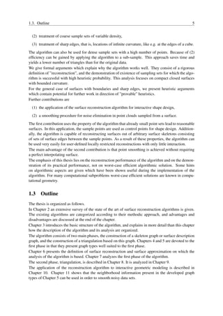
Figure 3.4: The reconstruction for the skull data set: intermediate stages of the reconstruction and the final result.
The overall approach of the algorithm follows the general principle of augmenting an initial SDG
by edges and triangles so that at any time the resulting cell complex is a reasonable fitting into the
data point set P . We have previously presented other solutions based on the same principle [Men95,
MM98a]. There, a longer sequence of graphs has been constructed before the algorithm has switched
to triangles. The advantage of the algorithm presented here is that the sequence of graphs has been
reduced to one graph, due to a quite general concept of environment graphs.
The algorithm is complemented by an analysis of its reconstruction behavior. For this purpose we
first give a precise definition of “reconstruction”. The definition is based on the concept of nearest-
neighbor (NN) image. It roughly tells that a mesh M is a reconstruction of a given surface S if the
NN-image of M on S is non-self-intersecting. Then, conditions on the sample point sets are derived
which are favorable in order that the mesh constructed by our algorithm is a reconstruction. These
conditions are used to demonstrate that a given sample set can be augmented to a sample set for which
our algorithm yields a reconstruction for closed surfaces without boundary of limited curvature, with
high heuristic probability.
The philosophy of NN-embedding is subject of Chapter 6. The analysis is described in Chapter 7 for
the SDG-phase, and in Chapter 9 for the phase of triangulation. Additional heuristic arguments for the
favorable behavior of the algorithm in interactive modeling environments are presented in Chapter 10.
Chapter 11 shows that the neighborhood information of the SDG can be used to smooth noisy data
sets.](https://image.slidesharecdn.com/surfacereconstructionrobertmenclphdthesis-130112202114-phpapp01/85/Reconstruction-of-Surfaces-from-Three-Dimensional-Unorganized-Point-Sets-Robert-Mencl-PhD-Thesis-35-320.jpg)

![Chapter 4
The Euclidean Minimum Spanning Tree
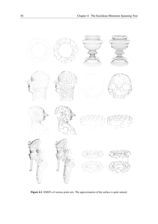
In this chapter a number of properties of the EMST are compiled which underline the observation
that the Euclidean minimum spanning tree (EMST) is a useful skeleton for surface-oriented interpo-
lation of surfaces from a set of scattered points, as illustrated in Figure 4.1. Furthermore, algorithmic
considerations concerning the calculation of the EMST are presented.
4.1 The Euclidean Minimum Spanning Tree – Definition and Properties
In the following we assume that the reader is familiar with the basic terminology of graph theory, like
it is e.g. described in [PS85, Ede87]. Briefly, a graph G = (V, E) consists of a set V of vertices and
a set E of edges. The edges are defined as pairs of vertices. A path in a graph G is a sequence of
different vertices so that any two consecutive vertices are connected by an edge. A graph is connected
if there is a path between any two of its vertices. A cycle is a closed path, that is, its first and last
vertices coincide. A tree is an acyclic connected graph, that is, a graph without cycles.
The Euclidean minimum spanning tree is defined as follows.
Definition 4.1 (Euclidean minimum spanning tree) Let P = {p1 , . . . , pn } be a finite set of points
in d-dimensional space. The Euclidean minimum spanning tree (EMST) of P is a tree that connects
all points of P with edges so that the sum of its Euclidean edge lengths is minimum.
The set of all minimum spanning trees of P is denoted by EMST (P ).
Theorem 4.2 (Uniqueness of the EMST) If the Euclidean distances between the points of a given
finite point set P are pairwise distinct, then the EMST is unique, that is, |EMST (P )| = 1.
Proof: For simplicity, let in the following the union of a graph H = (P, E) with an edge e, H ∪ e, be
defined as (P, E ∪ {e}). The difference H − e is defined analogously.
Now, let H = (P, E) and K = (P, E ′ ) be two different EMSTs of P . The edges in H and K are
sorted in order increasing edge length.
Let eH be the first of these edges that is in one EMST and not in the other. W.l.o.g. let eH be in H but
not in K. This means, that every edge with edge length less than eH is in both or neither of the trees
H, K.
Consider the tree K ∪ eH . Adding an edge to a tree always creates a cycle, so that K ∪ eH must
contain at least one cycle. By removing any edge of this cycle we again get a tree. By definition both
trees H, K do not contain any cycles. This means that there must be at least one edge eK in the cycle
of K ∪ eH which was in K but not in H. We remove that edge eK from K ∪ eH so that we get a new
tree L := K ∪ eH − eK .
Because eH was the shortest edge in one tree but not in the other, and because all distances between
the points are pairwise distinct, eK is longer than eH and cannot be of equal length.
29](https://image.slidesharecdn.com/surfacereconstructionrobertmenclphdthesis-130112202114-phpapp01/85/Reconstruction-of-Surfaces-from-Three-Dimensional-Unorganized-Point-Sets-Robert-Mencl-PhD-Thesis-37-320.jpg)

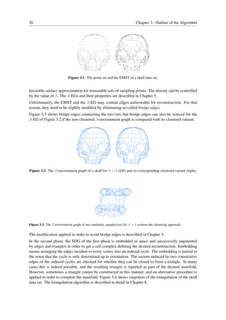
![32 Chapter 4: The Euclidean Minimum Spanning Tree
The consequence of Theorems 4.4 and 4.5 is that each leaf point of an EMST is connected with its
nearest neighbor.
The opposite of Theorem 4.4 is not true. If two points are connected by an EMST edge, the points are
not necessarily the nearest neighbors of each other, as proven in Theorem 4.6.
pnn(i) p
nn(j)
pj
p
i
Figure 4.3: Point pi is connected with pj in the EMST but no point of {pi , pj } is the nearest neighbor of the
other one. Note that pi pj is the nearest neighbor edge between the EMST subtrees ({pi , pnn(i) }, {pi pnn(i) }) and
({pj , pnn(j) }, {pj pnn(j) }).
Theorem 4.6 (Property of EMST edges) Let pi pj be an edge of the EMST of P . Then pi is not
necessarily the nearest neighbor of pj and vice versa.
Proof: Figure 4.3 shows a 2D configuration where a point pi is connected with pj but is not its nearest
neighbor.
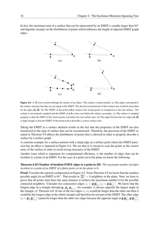
Although Theorem 4.6 holds, all edges of an EMST connect subtrees of the EMST. These EMST edges
represent the nearest neighbor connection between these subtrees. In fact, each edge of the EMST is
in some sense a nearest neighbor edge (between subtrees) where single points can be considered as
trivial subtrees of the EMST (cf. Theorem 4.7 and Algorithm 4.1).
Theorem 4.7 (Prim [Pri57]) Let G = (P, E) be a graph with weighted edges and let {P1 , P2 } be a
partition of the set P . Then there is a minimum spanning tree of G which contains the shortest among
the edges with one end point in P1 and the other in P2 .
Proof: See [Pri57] or [PS85].
The preceding theorems show that the edges of an EMST connect points that lie close together in
space. On the other hand, it can be expected for a reasonably sampled surface that the point density
on the surface is higher than anywhere else in the surrounding space. In particular for non-convex
surfaces and objects consisting of more than one component, points lying far apart from each other
in space are unlikely to be neighboring on the surface. Furthermore, if it is necessary to reconstruct
very small and detailed surface structures, the point density at those areas should be higher than at
parts with less detail. With respect to these considerations the EMST turns out to be very suitable as
a surface-approximating skeleton. Figure 4.1 illustrates this observation at several examples. We can
observe at these examples that the EMST follows the shape of the object in a quite natural manner.
Another type of graph having the property of short edges are the Nearest-Neighbor Graphs (NNG)
[Vel94]. The nearest neighbor graph of a finite point set P connects each of its points to its nearest
neighbor(s). According to Theorem 4.4, the NNG is a subgraph of the EMST. A disadvantage of the
NNGs is that, in contrast to the EMST, they are in general not connected.
Since we here investigate the properties of EMSTs as surface approximants it is necessary to determine
the sharpest possible turn between two consecutive edges. For this purpose we calculate the minimum
angle between two adjacent edges in the EMST. In order to do this we first need a consideration on
the angles inside a triangle which is analyzed in the following theorem.](https://image.slidesharecdn.com/surfacereconstructionrobertmenclphdthesis-130112202114-phpapp01/85/Reconstruction-of-Surfaces-from-Three-Dimensional-Unorganized-Point-Sets-Robert-Mencl-PhD-Thesis-40-320.jpg)
![4.1. The Euclidean Minimum Spanning Tree – Definition and Properties 33
Theorem 4.8 (Longest edge property in a triangle) Let t be a triangle with edges ea , eb , ec where
a = l(ea ), b = l(eb ), c = l(ec ) are the lengths of these edges. Furthermore, let α, β, γ be the angles
that are opposite to the edges ea , eb , ec . We assume that γ = max(α, β, γ) is the largest angle in the
triangle. Then, c = max(a, b, c) and ec is the longest edge in t.
Proof: From the sine theorem [BS87] we know that
a b c
= = . (4.1)
sin(α) sin(β) sin(γ)
Additionally, we know that for 0◦ ≤ δ ≤ 180◦ , the equation
sin(180◦ − δ) = sin(δ) (4.2)
holds.
W.l.o.g. we assume that γ with γ = max(α, β, γ) is the largest angle. We have to show that in that
case c ≥ a and c ≥ b holds. It is sufficient to show that c ≥ a because the sequence of equations for b
will be the same. Using Equation 4.1 we have
sin(γ)
c=a· .
sin(α)
Obviously, because of 180◦ = α + β + γ holds, the value γ must be larger or equal to 60◦ if γ =
max(α, β, γ). After these considerations we can make a case distinction.
For 60◦ ≤ γ ≤ 90◦ we obtain
sin(γ)
≥ 1
sin(α)
because γ ≥ α, α ≤ 90◦ and sin(γ) ≥ sin(α).
In the case of 90◦ < γ ≤ 180◦ we get
sin(γ) sin(180◦ − (α + β)) sin(α + β)
c=a· =a· =a·
sin(α) sin(α) sin(α)
by using Equation 4.2 and because of (α + β) ≤ 90◦ and sin(α + β) > sin(α). Therefore,
sin(α + β)
≥ 1
sin(α)
implying c > a. The same cases appear for the comparison of b with c.
A result of Theorem 4.8 is that the EMST maximizes the angles between adjacent edges because of
its minimum length property.
Using the result of the previous theorem, the minimum angle in an EMST can now be calculated.
Theorem 4.9 (Minimum angle in the EMST) Let P be a finite point set in d-dimensional space.
The minimum angle between two adjacent edges of EM ST (P ) at an arbitrary point pi ∈ P is 60◦ .
Proof: Let G = (P, E) = EM ST (P ) be the EMST of a finite point set P . Consider two arbitrary
edges e1 = pi pj , e2 = pi pk of G that are incident to an arbitrary point pi ∈ P . If e1 , e2 enclose
an angle γ less than 60◦ , then it is not the largest angle in the triangle t = △(pi , pj , pk ) because
180◦ = α + β + γ where α, β are the angles that are opposite to e1 , e2 in t. From Theorem 4.8
we know that the largest angle in t is opposite to the longest edge. Therefore, either e1 or e2 is the
longest edge in t. This means that the points pi , pj , pk can be connected with two other edges that
have a lower edge length sum than l(e1 ) + l(e2 ). The consequence is that there also exists an edge set
E ′ with lower edge length sum than E that connects all points of P . This is a contradiction because
G = (P, E) is an EMST.](https://image.slidesharecdn.com/surfacereconstructionrobertmenclphdthesis-130112202114-phpapp01/85/Reconstruction-of-Surfaces-from-Three-Dimensional-Unorganized-Point-Sets-Robert-Mencl-PhD-Thesis-41-320.jpg)
![4.1. The Euclidean Minimum Spanning Tree – Definition and Properties 35
pk pk
3 2
60 degrees
pk p p
i
4 k 1
p p
k k
5 6
Figure 4.5: The maximum number of EMST edges around a point of the given planar point set is 6. The distances between
consecutive points pki , pki+1 are equal to d(pi , pki ) for i ∈ {1, . . . , 6}. Provided that the distances to the middle point are
smaller only for numerical reasons, this EMST graph is the optimal structure. On the other hand, the shown EMST graph is
one of the possible EMST graphs for this point set.
is still 60◦ , and at least one of the angles in the (new possible) triangle induced by edges e1 , e2 with
non-equal length would have to be larger than 60◦ . Therefore, all points pkj must have equal distance
to pi .
In three dimensions the number of possible EMST edges around an arbitrary point in EM ST (P ) can
be higher.
Theorem 4.11 (Number of incident EMST edges to a point in 3D) The largest vertex degree, that
is, the number of incident edges of an EMST in 3D space is 12.
Proof: We place a number of edges e1 , . . . , ek with arbitrary length at an arbitrary point pi with
pairwise angles of minimum 60◦ . W.l.o.g. let el be the shortest edge at pi with scaled length 1. We
1
place spheres of radius 2 at pi and at each so-called anchor point on e1 , . . . , ek with distance 1 to pi .
Because each pairwise angle is at minimum 60◦ the spheres cannot penetrate each other. They can
only touch each other which is the case if the angle of two neighboring edges is exactly 60◦ since pi
and the two anchor points form an equally-sided triangle (see Figure 4.6). The number of edges with
spheres at their anchor points that can be placed around pi without penetrating each other corresponds
to the problem of how many spheres with equal radius (= 1 ) can be placed at a center sphere at pi .
2
This problem is solved in [SvdW53, Lee56, CS88] and its number is limited to 12. 1
Now, we have to show that there exists at least one configuration of edges at pi which is an EMST.
If all edges are replaced with edges that connect only the anchor points with pi this is at least one
possible configuration which is an EMST. This is because each anchor point has at least a distance of
1 to each other anchor point, the same distance as to pi . Therefore, the edges at pi represent one of
the possible EMSTs for the anchor points and pi .
In Theorem 4.11 the maximum number of edges around a point pi in the EMST has been computed.
In the ideal case this value is 12 but in practice it can be expected to be much lower. Especially, if the
1
The oldest proofs appeared in the nineteenth century [Ben74, Hop74, G¨ n75]. Other approaches can be found in
u
[Boe52] and [Was78]. The whole problem area is also known as the kissing number problem, cf. [CS88].](https://image.slidesharecdn.com/surfacereconstructionrobertmenclphdthesis-130112202114-phpapp01/85/Reconstruction-of-Surfaces-from-Three-Dimensional-Unorganized-Point-Sets-Robert-Mencl-PhD-Thesis-43-320.jpg)
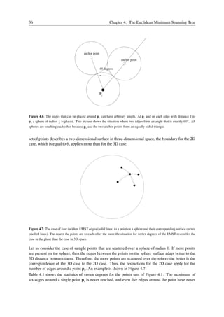
![4.2. Computational Issues 37
# of vertices of degree k in the EMST
torus cup head skull puppet cap pharaoh tori
# points 310 2650 1487 698 695 371 2286 620
k=1 76 325 262 167 177 83 446 145
k=2 163 2020 975 379 356 211 1413 337
k=3 68 287 240 139 149 73 410 133
k=4 3 18 10 13 13 4 17 5
# edges 309 2649 1486 697 694 370 2285 619
Table 4.1: Statistics of vertex degrees for the EMSTs of our example point sets. The vertex degree is much lower than the
theoretic upper bound of 3D EMSTs. Even the bound of 6 for the vertex degree of the 2D case is not reached.
occurred in all of our examples. The maximum value here has been four, and in average we can expect
approximately two or three edges at a point.
However, for reasons of complexity the worst case has to be considered anyway. Here, if the max-
imum of 12 edges occurs then all surrounding points cannot have the same maximum vertex degree
[SvdW53]. There are several papers on this topic in which bounds are derived from the theory of
spherical packings in three-dimensional space which can be found in [CS88].
As a result, the number of EMST edges that are in average around a point can be expected equal to or
less than 4.
4.2 Computational Issues
The calculation of the EMST is a classical problem of computational geometry, and efficient algo-
rithms are known for it.
computation times in seconds
object # points
DT(P ) EM ST (P )
torus 310 1 0.03
cup 2650 11 0.32
head 1487 6 0.18
skull 698 3 0.08
puppet 695 3 0.08
cap 371 2 0.04
pharaoh 2286 10 0.29
tori 620 1 0.07
Table 4.2: The computation times of the Delaunay triangulation and the subsequent EMST calculation for our examples in
seconds on an SGI Octane R10000 at 250 MHz with 384 MByte of memory.
A frequent approach is to calculate the EMST out of the Delaunay triangulation of the point set,
because the EMST is a subgraph of the Delaunay graph [PS85]. The worst case time complexity
of the Delaunay triangulation is O(n2 ) in 3D space [Joe89, Joe91]. The computation of the EMST
out of a supergraph requires O(|E| log n) operations, where |E| denotes the number of edges in the
supergraph. The number of edges in the 3D Delaunay triangulation can be O(n2 ) in the worst case,
which results in O(n2 log n) for the EMST computation out of the Delaunay triangulation. Calculation](https://image.slidesharecdn.com/surfacereconstructionrobertmenclphdthesis-130112202114-phpapp01/85/Reconstruction-of-Surfaces-from-Three-Dimensional-Unorganized-Point-Sets-Robert-Mencl-PhD-Thesis-45-320.jpg)
![38 Chapter 4: The Euclidean Minimum Spanning Tree
of the EMST is possible by using one of the optimal spanning tree algorithms of graph theory, for
example that of Kruskal [PS85].
The computation times for our examples can be found in Table 4.2. For the calculation of the Delaunay
triangulation the software of M¨ cke has been used [M¨ c93b, M¨ c93a, EM94].
u u u
Algorithm 4.1 Computation of EM ST (P )
Input: Point set P = {p1 , . . . , pn }.
Operation: Compute the EM ST of P .
Let Gi := ({pi }, ∅) be the initial one-node-trees for i = 1, . . . , n.
Let G := {G1 , . . . , Gn } be the set of all trees.
while ( |G| > 1 ) do
foreach ( Gj ∈ G with j ∈ { 1, . . . , |G| } ) do
Determine the nearest neighbor tree Gk ∈ G of Gj .
Let pr ps be the shortest connecting edge between Gj and Gk .
G′ := Gj ∪ ({pr , ps }, {pr ps }) ∪ Gk .
G := (G − {Gj , Gk }) ∪ {G′ }.
end
end
Output: EM ST (P ).
Another possibility is to calculate the EMST directly. A particularly suited spanning tree algorithm
for that purpose is that of Bor˚ vka. According to Ottmann & Widmayer [OW90] the algorithm of
u
Bor˚ vka [Bor26] is reported to be the historically first algorithm for the computation of a minimum
u
spanning tree. It is shown in Algorithm 4.1. The union of graphs G1 = (P1 , E2 ) and G2 = (P2 , E2 )
used in the algorithm is defined as G := (P1 ∪ P2 , E1 ∪ E2 ). At the beginning of the algorithm, an
initial forest of one-node-trees is established. Each vertex of P defines one tree of that forest. Then
for each tree Gj its nearest neighbor tree Gk is computed, which is the tree that contains the point ps
not in Gj which has the shortest Euclidean distance to the nearest point pr of Gj . Both trees are then
merged into one single tree, so that the number of all trees is decreased by one. This tree merging
process is repeated until the set of these trees has reduced to one tree.
Prim’s algorithm [Pri57] is a special case of the algorithm of Bor˚ vka. There, the process starts with
u
a single tree defined by an arbitrary vertex node. This initial tree is then sequentially extended by its
nearest neighbor connection to a new vertex, that is not already part of the current tree. As before, the
process is finished if all vertices have been connected to one tree.
4.3 Discussion
This chapter has dealt with the properties which make the EMST useful as an initial skeleton of a
surface. Experimental examples have demonstrated the favorable behavior of the EMST. Furthermore,
algorithmic aspects concerning the calculation of the EMST have been treated.](https://image.slidesharecdn.com/surfacereconstructionrobertmenclphdthesis-130112202114-phpapp01/85/Reconstruction-of-Surfaces-from-Three-Dimensional-Unorganized-Point-Sets-Robert-Mencl-PhD-Thesis-46-320.jpg)
![Chapter 5
Environment Graphs
In the previous chapter we have seen that the EMST can serve as a good surface approximation.
However, in Figure 5.1 we can notice that the torus ring is not closed with edges because of the
minimum length property of the EMST (cf. Chapter 4). As consequence, in this chapter we consider
more dense graph schemes, the so-called environment graphs which extend the concept of the EMST
and preserve to a large extent the favorable surface approximation properties of the edges which we
could observe for the EMST. Furthermore, we cope with the problem of bridge edges which may
connect parts of a surface over a large distance in an undesirable manner, as could be noticed for
example for the double torus in the preceding chapter, cf. Figure 4.1.
Figure 5.1: The point set and the EMST of a torus that consists of rings of points.
5.1 Environment Graphs
The following definition describes a very general concept of environment graphs which can be spe-
cialized to several known classes of graphs.
Definition 5.1 (Environment graph (EG)) Let U be a function that assigns to every line segment s in
the d-dimensional space I d a set U (s) of environments of s. The U -edge-environment graph (U -EG)
R
of a finite set of points in I d is a graph with vertex set P , whose edge set consists of all those line
R
segments e induced by pairs of points in P for which there exists an U (e) ∈ U (e) with U (e) ∩ P = ∅,
that is, the U -environment of e does not contain any point of P .
A typical example of an EG is the Delaunay graph whose edges are just those line segments of its
vertex set which have an empty surrounding sphere [PS85, Ede87]. In that case, U (s) is the set of all
surrounding spheres of s.
39](https://image.slidesharecdn.com/surfacereconstructionrobertmenclphdthesis-130112202114-phpapp01/85/Reconstruction-of-Surfaces-from-Three-Dimensional-Unorganized-Point-Sets-Robert-Mencl-PhD-Thesis-47-320.jpg)

![5.1. Environment Graphs 41
An implication of the theorem is that EMSE-graphs should be triangle-free with high probability.
Several properties of the EMST which are of local nature can also be found for the EMSE-graph.
Theorem 5.7 (Local EMSE-graph properties) Let P be a finite point set in I d and p, q ∈ P .
R
(1) Let p be a leaf point of the EMSE-graph of P , that is, a point with exactly one incident edge,
which is connected with a point q. Then q is the nearest neighbor of p.
(2) Let pq be an edge of the EMSE-graph of P . Then p is not necessarily the nearest neighbor of q
and vice versa.
(3) The minimum angle between two adjacent EMSE-graph edges at an arbitrary point p of the
graph is 60◦ .
(4) The maximum number of edges incident to a point of an EMSE-graph of a point set in the plane
is 6.
(5) The largest vertex degree, that is, the number of incident edges, of an EMSE-graph in 3D space
is 12.
Proof: Analogously to the EMST case, cf. Chapter 4.
The suitability of the EMSE-graph as a framework of surface interpolation lies in the fact that the
EMSE is not able to ”escape” into the empty space as the surrounding spheres of the Delaunay tri-
angulations can. Figures 5.2 and 5.3, left column, show the Delaunay triangulation of our series of
sample data sets. In the second column from the left, the corresponding EMSE-graphs are depicted.
Here the question arises for environment graphs induced by spheres which are prevented to escape.
An immediate possibility is that the corresponding environment of an edge is bounded by the unique
sphere having the edge as its diameter. This type of graph is well-known as Gabriel graph [GS69]
which has been preferably used in the plane. Both graph classes, the EMSE-graphs and the Gabriel
graphs, can be seen in the much wider framework given by the concept of β-environment graphs.
Definition 5.8 (β-environment graph (β-EG)) Let e = pq, p, q ∈ I 3 be a line segment, and H a
R
3
plane in I containing e.
R
For β ≥ 0, let p′ , q′ be points on the line induced by e located symmetrically with respect to its center
m := 1 (p + q), that is
2
p′ = βp + (1 − β)m,
q′ = βq + (1 − β)m.
Let Eβ (e) be the intersection of the disc in H with center p′ through q with the disc in H with center
′
q ′ through p, cf. Figure 5.4 (left).
For β < 0, let p′ , q′ be points on the perpendicular line in H through the center m of an edge e = pq
located symmetrically with respect to its center, with
||p′ − m|| = ||q′ − m|| = −β · ||q − p||,
′
where · denotes the Euclidean norm. The environment Eβ (e) is defined as the intersection of the
disc with center p ′ through p and q with the disc with center q′ through p and q, cf. Figure 5.4 (right).
′
Let Eβ (e) be the set of points obtained by rotating Eβ (e) around e. Eβ (e) is called the β-environment
of e. The environment graph with β-environments as environments is called β-environment graph. In
2D space H is replaced with the 2D space and Eβ (e) := Eβ (e). ′](https://image.slidesharecdn.com/surfacereconstructionrobertmenclphdthesis-130112202114-phpapp01/85/Reconstruction-of-Surfaces-from-Three-Dimensional-Unorganized-Point-Sets-Robert-Mencl-PhD-Thesis-49-320.jpg)
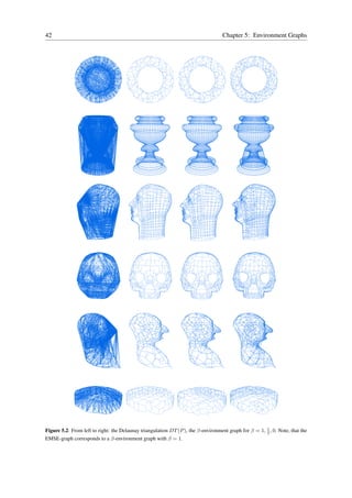
![5.1. Environment Graphs 43
Figure 5.3: From left to right: the Delaunay triangulation DT (P ), the β-environment graph for β = 1, 1 , 0. Note, that the
2
EMSE-graph corresponds to a β-environment graph with β = 1.
Sometimes we also will use Eβ (p, q) = Eβ (e) as another notation of the β-environment of an edge
e = pq.
In 2D space, the value β = 0 yields the Gabriel graph, in 2D and 3D space β = 1 yields the EMSE-
graph.
In two dimensions, the β-environment graphs for β ≥ 0 correspond to the lune-based neighborhood
graphs of Kirkpatrick and Radke for their β ≥ 1, for β ≤ 0 to their circle-based neighborhood graphs
for their β between 0 and 1 [KR85, Rad88]. Recently, Rao [Rao98] has independently generalized the
neighborhood graphs to higher dimensions. Up to the β-parameterization, our β-environment graphs
are the same as his lune-based neighborhood graphs.
1
Figures 5.2 and 5.3 show β-EGs for β = 1, 2 , and 0 of our sample data sets. We can notice that
also in the 3D-case the resulting graph yields a reasonable, almost planar approximation. The number
of ”crossing” edges is very small, and decreases with increasing β. Figure 5.5 shows the edges of
1
β-environment graphs for β = − 2 which additionally are Delaunay edges. Even with this restriction,
many edges useless for reconstruction are delivered. On the other hand, the chance seems to be good
that the desired mesh is a subset of this graph. Based on this observation it might be possible to find a
surface reconstruction algorithm that works by eliminating the superfluous edges from the graph.
As we can see from our examples, the number of edges in the β-EG decreases with increasing β.
Some statistics of vertex degrees, that is, the number of points with k incident edges in the β-EGs for
1
β = 1, 2 , 0 are shown in Tables 5.1, 5.2, 5.3.
An interesting observation is that β-environment graphs have a hierarchical structure.
Theorem 5.9 (Subgraph hierarchy of the β-EG) For a given finite point set P in 3D space, if β1 >
β2 , the β1 -EG of P is subgraph of the β2 -EG of P .
Proof: The property results from the observation that Eβ2 (p, q) ⊂ Eβ1 (p, q).](https://image.slidesharecdn.com/surfacereconstructionrobertmenclphdthesis-130112202114-phpapp01/85/Reconstruction-of-Surfaces-from-Three-Dimensional-Unorganized-Point-Sets-Robert-Mencl-PhD-Thesis-51-320.jpg)
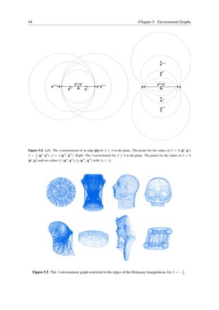


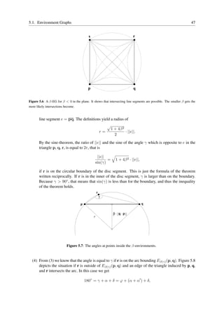

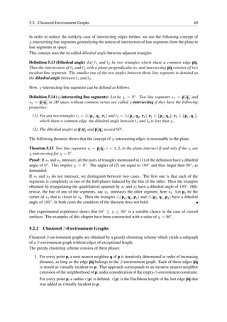

![5.3. Computational Issues 51
have an empty β-environment. This radius is a first estimation for the length of edges that deliver a
good surface approximant. Therefore, all edges pq with empty β-environment and length less than or
equal to r(p) can be stored as virtual edges.
In the second step, the radii of points in the neighborhood of each point are used to apply a controlled
enlargement of these radii. Therefore, all points p, q with intersecting spheres are updated by the
maximum of r(p) and d(p, q) if the β-environment Eβ (p, q) of the edge between them is empty of
points. Additionally, all points q that are inside a sphere of a point p are updated with the maximum
of r(q) and their distance to the border of the sphere of p. Since the update of some radii might
cause new intersections with other spheres, the second step is repeated until no more update takes
place. The generated radii of the second step are used to determine another set of virtual edges that are
established between points p, q with intersecting spheres and whose connecting edge pq has an empty
β-environment. Because all radii have been generated with respect to the distribution of points in the
neighborhood of each point, the total length of each virtual edge is limited. Therefore, the virtual
edges can be considered as good surface approximants. An analysis that the limitation of the length
of graph edges indeed delivers “good surface approximants” is given in the next two chapters.
The third and last step is used to determine the order how the virtual edges of all points are inserted as
final edges of the graph. Here, the edges are considered in order of increasing length, since we assume
that shorter edges are better surface approximants than longer ones.
The algorithm should work well if at a vertex p with a bridge edge in its β-environment graph, vertices
not adjacent to p are in a neighborhood of a radius far less than the length of the edge.
Algorithm 5.1 summarizes this procedure in pseudocode notation.
1
Figures 5.9 and 5.10 show the resulting clustered β-environment graphs of our test cases for β = 1, 2 ,
and 0. As can be noticed, the number of long edges has significantly reduced. The statistics of vertex
degrees of these graphs, that is the number of incident edges to a point, are given in Tables 5.4, 5.5,
5.6. The difference of the number of edges of the clustered β-environment graphs in comparison to
the complete β-environment graphs are given in Table 5.7.
5.3 Computational Issues
The computation of the planar relatives of our β-environment graphs, the β-neighborhood graphs, has
been intensively investigated in the thesis of Rao [Rao98]. Rao also has presented an approach to the
calculation of special three-dimensional cases, namely β-environment graphs for β ≥ 1.
The straightforward approach to the calculation of the β-environment graph is to check all pairs of
points for whether they have an empty environment. This approach may be feasible for very small
point sets, but cannot be applied to larger sets. A better alternative is the filtering approach. The
filtering approach uses a reasonable supergraph G′ of the desired graph G, and removes those edges
from G′ which do not satisfy the empty-environment criterion.
A natural supergraph for β ≥ 0 is the Delaunay triangulation. The Delaunay triangulation often works
quite well, but it may have O(n2 ) edges in 3D space in the worst case, n the number of vertices.
An idea of constructing an other type of supergraph, the sector supergraph, can be found in the work
of Yao [Yao82, Rao98]. For every point p, the space is subdivided into pyramidal sectors R with apex
p. If the sectors are sufficiently narrow, it can be shown that every point in R which is more distant
than a certain bound dependent on the distance of the nearest neighbor of p in the sector does not have
an empty environment. The supergraph G′ contains all connections from p to those points in R as
edges which do not satisfy this criterion. For β ≥ 1, Yao has shown that the sector supergraph only
contains O(n) edges. The edges of the supergraph can be determined by nearest-neighbor search as
described in Appendix B.](https://image.slidesharecdn.com/surfacereconstructionrobertmenclphdthesis-130112202114-phpapp01/85/Reconstruction-of-Surfaces-from-Three-Dimensional-Unorganized-Point-Sets-Robert-Mencl-PhD-Thesis-59-320.jpg)
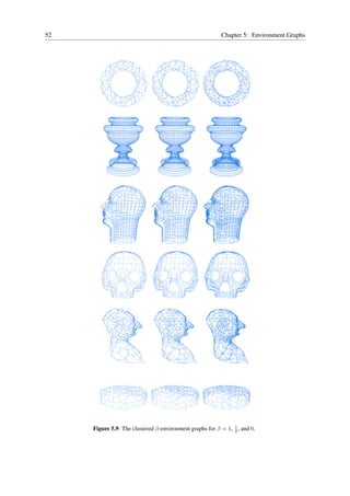
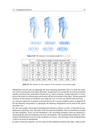
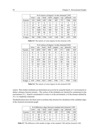


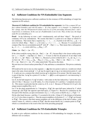
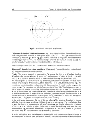
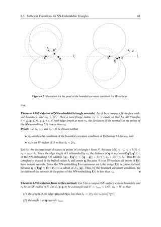
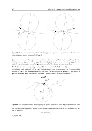
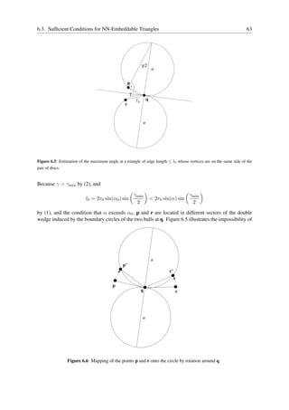


![66 Chapter 6: Approximation and Reconstruction
n n
n ( t2)
n ( t2)
n ( t1 )
n ( t1 )
Figure 6.8: Cases of the dihedral angle between two triangles.
(1) have edge lengths less than r0 ,
(2) have angles in the interval (γmin , γmax ),
(3) share a common edge.
Then the dihedral angle between t1 and t2 is in the interval (180◦ − 2α0 , 180◦ ] or in the interval
[0◦ , 2α0 ).
Proof: Two triangles which share a common edge also have a common vertex p. By Lemma 6.11,
the angles α(n(p), n(ti )), i = 1, 2, between the surface normal n(p) at p and the normals n(ti ),
i = 1, 2, of the triangles are less than α0 . By considering the metric of shortest distances on the
unit sphere, that implies that the angle |α(n(t1 ), n(t2 ))| between the normals of the triangles satisfies
|α(n(t1 ), n(t2 ))| ≤ |α(n(p), n(t1 ))| + |α(n(p), n(t2 ))| < 2α0 .
From the two possible orientations of the normals, two cases concerning the dihedral angle arise
(cf. Figure 6.8). The bound on the normals implies the two bounds on the dihedral angles of the
corollary.
n ( t 2)
n (p)
n ( t1)
p
Figure 6.9: Proof of the size of the dihedral angle by transforming the orientation of the surface to the approximating
triangle.
For a reasonable triangulation, only the case of dihedral angles in (180◦ − 2α0 , 180◦ ] is of interest.
Corollary 6.14 (Dihedral angle bound) Let S be a compact SF-surface without boundary. Let 0◦ <
γmin < γmax := 180◦ − γmin < 180◦ , 0◦ < α0 < 90◦ , and r0 as in Theorem 6.12. Let t1 and t2 be
two triangles incident to a common edge, which
(1) have edge length less than r0 ,](https://image.slidesharecdn.com/surfacereconstructionrobertmenclphdthesis-130112202114-phpapp01/85/Reconstruction-of-Surfaces-from-Three-Dimensional-Unorganized-Point-Sets-Robert-Mencl-PhD-Thesis-74-320.jpg)
![6.4. Sufficient Conditions for NN-Embeddable Pairs of Triangles 67
(2) have angles in the interval (γmin , γmax ),
(3) are together NN-embeddable in S.
Then the dihedral angle between t1 and t2 at the common edge is in the interval (180◦ − 2α0 , 180◦ ].
Proof: The NN-embedding of the triangles t1 and t2 on S consists of two surface triangles which are
disjoint up to parts of their boundaries. We orient the edges of the two surface triangles so that they
appear counter-clockwise oriented from the side of the surface on which the normal vector at one of
the end points p of the common edge is directed. We transfer the orientation to t1 and t2 , and consider
the normals n(t1 ) and n(t2 ) directed so that their angles with the normal n(p) of p are less than α0 .
Then t1 and t2 appear counter-clockwise oriented if viewed from the side of their normals. The angle
between n(t1 ) and n(t2 ) is less than 2α0 . Figure 6.9 depicts the resulting configuration. As can be
clearly noticed the only possibility of a configuration of that type is that one with the dihedral angle in
the interval (180◦ − 2α0 , 180◦ ].
Lemma 6.15 Let S be a compact SF-surface without boundary. Further, let t1 and t2 be two triangles
with vertices on S, incident to a common edge, with dihedral angle larger than 180◦ − δ0 > 90◦ ,
δ0 > 0◦ , n(t1 ) and n(t2 ) the normals of t1 and t2 , respectively, p1 ∈ t1 , p2 ∈ t2 . Then the angle
between the vectors p2 − p1 and n(t2 ), and between p1 − p2 and n(t1 ), respectively, exceeds 90◦ − δ0 .
Proof: The smallest angle between p2 − p1 and n(t2 ) is achieved if p2 is on the common edge of t1
and t2 , and p2 − p1 perpendicular to that edge. In that case, the angle between p2 − p1 and n(t2 ) is
equal to 90◦ − δ0 . The assertion for p1 − p2 and n(t1 ) holds for reasons of symmetry.
Now we can formulate a result on intersection-free embeddings of two adjacent triangles.
Theorem 6.16 (Sufficient condition for NN-embeddable pairs of triangles) Let S be a compact SF-
surface without boundary, 0◦ < γmin < γmax := 180◦ − γmin < 180◦ , δ0 > 0◦ . Then an SF-radius
r0 > 0 of S exists so that all triangles ti = △(pi , qi , ri ), pi , qi , ri ∈ S, i = 1, 2, for which
(1) the edge length of t1 and t2 is bounded by r0 ,
(2) the angles of t1 and t2 at q1 and q2 , respectively, satisfy γmin < γ < γmax ,
(3) the dihedral angle between t1 and t2 along a common edge is larger than 180◦ − δ0 > 90◦ ,
are NN-embeddable, and their NN-images f(t1 ) and f(t2 ) are disjoint, up to the NN-image of their
common edge.
Proof: From Theorem 6.8 we know that for a given α1 > 0◦ , r0 > 0 exists so that for all triangles
′
t1 , t2 satisfying (1) and (2) the deviation of the normals at the points of the NN-images f(t1 ) and f(t2 )
′
is less than α1 . We set r1 := r0 .
From Theorem 6.9 we know that for a given α2 > 0◦ , r0 > 0 exists so that, if (1) and (2) are satisfied,
′
the angle between the surface normal n(qi ) at qi and the normal n(ti ) of the triangle ti , i = 1, 2, does
not exceed α2 . We set r2 := r0 . ′
′
From Theorem 6.5 we know that an r0 > 0 exists so that all triangles t1 , t2 satisfying (1) and (2) are
NN-embeddable. We set r3 := r0 ′.
Let α1 = α2 := (90◦ − δ0 )/2, r0 := min{r1 , r2 , r3 }. For this r0 , the assertion of the theorem that t1
and t2 are NN-embeddable holds. Furthermore, the angle between n(ti ), i = 1, 2, and any normal on
f(ti ) is less than 90◦ − δ0 < 90◦ . On the other hand, by Lemma 6.15, the directions of lines between
points on ti deviate by more than 90◦ − δ0 from n(ti ), i = 1, 2. This contradiction implies that none
of the lines along the normals on f(ti ), i = 1, 2, intersects t1 and t2 simultaneously, except possibly
on the common edge of t1 and t2 . Thus the NN-embeddings are disjoint, up to the common edge.](https://image.slidesharecdn.com/surfacereconstructionrobertmenclphdthesis-130112202114-phpapp01/85/Reconstruction-of-Surfaces-from-Three-Dimensional-Unorganized-Point-Sets-Robert-Mencl-PhD-Thesis-75-320.jpg)

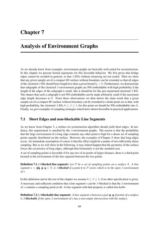
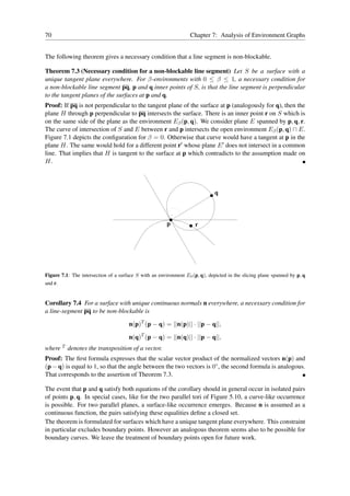
![7.1. Short Edges and non-blockable Line Segments 71
The stated condition is not sufficient because the environment may intersect the surface elsewhere.
If we assume the given surface not having non-blockable line segments, the following theorem shows
the existence of a sampling set for which the 0-environment graph does not have long edges.
Theorem 7.5 (Existence of length-bounding sampling sets) Let S be a compact surface without
boundary which has just blockable line segments, and P be a finite set of sample points taken from S.
Then, for every l0 > 0, P can be extended to a finite point set P ′ of points of S so that all line segments
s with length l(s) > l0 are β-blocked by a point in P ′ , 0 ≤ β ≤ 1. P ′ is called a blocking set.
Any further finite extension of P ′ does not violate this property.
Proof: The proof of existence uses the theorem of finite coverings of compact sets [Ber63, Kur68].
Let M be the set of all line segments between two points of the surface S. M is a compact set. We
consider M1 , the set of all line segments of length less than l0 . M1 is an open set, so that M2 :=
M − M1 is a compact set.
For every point r of S, we consider the set E(r) of all line segments s = pq of M2 for which r lies in
the interior of the intersection of the surface with the β-environment Eβ (p, q) of s. Note that r = p,
r = q. E(r) is an open set.
The sets E(r) cover M2 because every blockable line segment has a surface point in the interior of the
intersection of the surface with the diameter sphere.
Because M2 is compact (it is bounded because S is bounded), there exists a finite covering of M2 by
sets E(r). The points r of these sets define a blocking set P ′′ .
Because a superset of a blocking set is a blocking set, too, P ′ := P ∪ P ′′ is the desired set of the
theorem.
For a line segment s = pq with p, q ∈ P which has to be blocked, there is a point r ∈ P , r = p,
r = q, which blocks s. The reason is that, by definition, s is not in E(p) and not in E(q).
Corollary 7.6 Under the conditions of Theorem 7.5, for every finite super-set P ′′ of a blocking set P ′ ,
the edges e of the corresponding β-environment graph on P ′′ satisfy l(e) ≤ l0 .
Definition 7.7 (Samp1 -property) Let be l0 > 0, ε > 0, S a surface. A finite set P of points of S has
the Samp1 (l0 , ε)-property if every line segment s = pq, p, q ∈ S, has at least one of the following
properties:
(1) l(s) ≤ l0 ,
(2) n(p)T (p − q) > ||n(p)|| · ||p − q|| · (1 − ε),
n(q)T (p − q) > ||n(q)|| · ||p − q|| · (1 − ε).
That means that s is shorter than l0 , or lies close to line segments which satisfy the necessary condition
of non-blockable segments.
Corollary 7.8 (Existence of Samp1 -sample sets) Let S be a compact surface without boundary and
with continuous normals, which also may have non-blockable line segments, and P be a finite set of
sample points taken from S. For every l0 > 0 and ε > 0, P can be extended to a finite set P ′ which
has the Samp1 (l0 , ε)-property.
Proof: Let M3 be the set of line segments satisfying (2) of Definition 7.7. Then M4 := M − M3 is a
compact set which just has β-blockable line segments. For that set, Theorem 7.5 can be applied which
yields the existence of a suitable blocking set.](https://image.slidesharecdn.com/surfacereconstructionrobertmenclphdthesis-130112202114-phpapp01/85/Reconstruction-of-Surfaces-from-Three-Dimensional-Unorganized-Point-Sets-Robert-Mencl-PhD-Thesis-79-320.jpg)

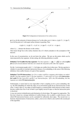
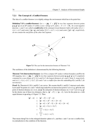
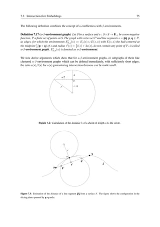
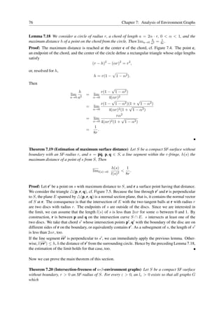
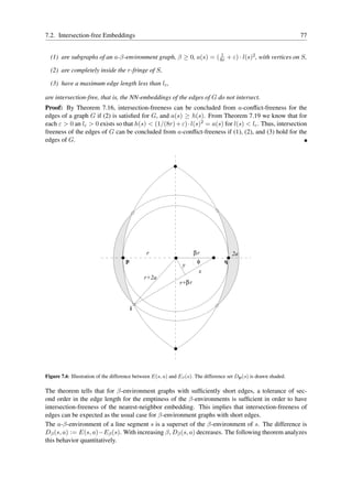
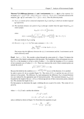
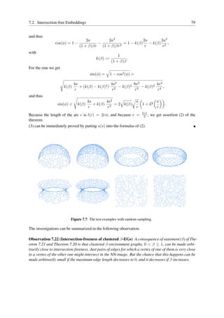
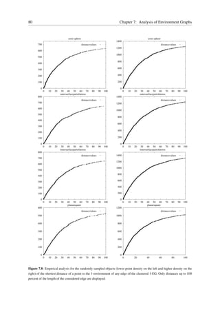
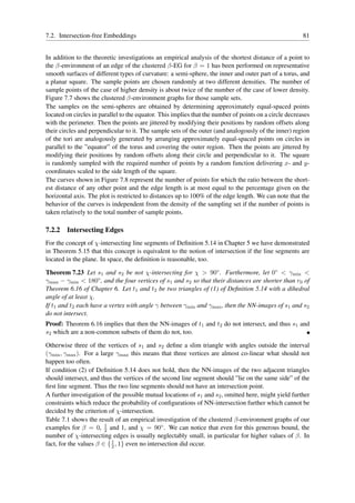
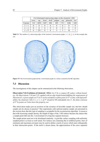
![7.3. Discussion 83
Figure 7.10: Left: the reconstruction out of the 1-environment graph. Right: the reconstruction with the marching cubes
algorithm.
between two consecutive intersection points by line segments may induce a mesh of loops with angles
of about 90◦ at two adjacent edges. The loops of such a mesh are usually quadrilaterals, and hence
have a constant number of edges. Furthermore, the diameter discs of the edges should in many cases
be empty of vertices, so that the 0-environment graph should contain many of them. Although the
restrictions for the 1-environment graph are higher than for the 0-environment graph, this can also be
achieved for this type of graph, as it can be seen in the example of the cup in Figure 5.9 of Chapter 5.
Another observation is that the edges delivered by the marching cubes algorithm from a spatial grid
sampling of a surface, are a subset of edges reconstructed by the 0-environment graph. The marching-
cubes (MC) algorithm [LC87] samples closed surfaces by a rectangular spatial grid. The vertices of
the grid are classified as interior or exterior with respect to the surface. From the vertex classification
of a cube of the mesh, a configuration of intersection of the surface with the cube is derived which
consists of one or more surface loops. These loops, or a triangulation of them are reported as a surface
approximation.
The MC-algorithm can also be seen as an edge-scan algorithm. The edges of the grid intersecting the
surface are determined. A sampling grid is proper if every edge contains at most one intersection point
with the surface. These intersection points define the loop configuration of a cube. The advantage of
that view is that the surfaces need neither be closed nor orientable. If the sampling is restricted to
cubes not traversed by the boundary of the surface, the MC algorithm yields an approximation of the
surface.
For SF-surfaces, due to their bounded curvature, the sampling grid of the marching cubes algorithm
can be chosen so dense that configurations with more than two sample points on an edge of a square
do not occur. Furthermore, the sampling grid can be chosen so dense that MC-configurations with
disconnected traversals or tubes do not occur, that is, every cube defines a single loop.
The diameter disc of an edge in the scan square in which the edge is located does not contain any
sampling point. The reason is that it only may intersect edges of the square, but those edges do not](https://image.slidesharecdn.com/surfacereconstructionrobertmenclphdthesis-130112202114-phpapp01/85/Reconstruction-of-Surfaces-from-Three-Dimensional-Unorganized-Point-Sets-Robert-Mencl-PhD-Thesis-91-320.jpg)

![Chapter 8
Triangulation
This chapter describes the second phase of the reconstruction algorithm, the triangulation, together
with new definitions required for its formulation.
8.1 The Algorithm
Algorithm 8.1 summarizes the approach of triangulation. The algorithm consists of two main steps, the
generation of a partial embedding, indicated by (1), and a phase of incremental triangulation, indicated
by (2). The goal of step 1 is the generation of very local embeddings of the surface description graph
G obtained from phase 1 of the reconstruction algorithm. Each local embedding concerns a vertex and
its incident edges in G. A local embedding of this type is achieved by defining a sorted arrangement
of the incident edges of the vertex. The local surface into which the vertex and its edges are embedded
is the “umbrella” of triangles obtained by closing every sector defined by two consecutive edges of
the arrangement by a chord. Usually the union of those local embeddings will not yield a manifold
surface, so that we do not necessarily use these triangles. A detailed investigation has to be performed
in order to decide whether a triangle of this type is used as part of the reconstructed surface. This
investigation is subject of step 2.
Step 2 processes the sectors obtained in step 1 according to a suitable priority. Depending on the
opening angle and the location of points and edges in the environment of the sectors, the algorithm
iteratively inserts new edges into graph G and adds triangles to the initially empty manifold M which
finally defines the reconstructed surface, remember Figure 3.4 of Chapter 3.
The details of the two steps are described in the following sections.
8.2 Generation of a Partial Embedding
In the first step, the originally purely combinatorial graph is partially embedded. Embedding of a
graph in principle means to find a surface in space of which the graph is a part. From combinatorial
topology we know that an embedding is uniquely defined by the sorted arrangement of the incident
edges at every vertex. Intuitively, if an embedding is given, two consecutive edges of the arrangement
at a vertex lie on a common face of the surface into which the graph is embedded. If sorted edge
arrangements at the vertices are given, the rule of face and thus of surface construction depends on
whether the embedded manifold should be orientable or not [Whi73].
In combinatorial topology the goal usually is to find a topological embedding so that the genus of the
embedding is minimized. In our setting, we can use the geometric information on the location of the
vertices in space for the definition of the arrangements π(v). The goal is to determine an optimally
flat arrangement of the incident edges of a vertex. Flatness is in principle measured by considering
85](https://image.slidesharecdn.com/surfacereconstructionrobertmenclphdthesis-130112202114-phpapp01/85/Reconstruction-of-Surfaces-from-Three-Dimensional-Unorganized-Point-Sets-Robert-Mencl-PhD-Thesis-93-320.jpg)
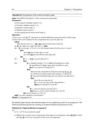
![8.2. Generation of a Partial Embedding 87
• 180◦ > δc > 0◦ .
Then
• Z(π(p)) denotes the maximum number of consecutive edges so that the triangles induced by
every subsequent pair of them have a dihedral angle in (δc , 180◦ ].
• Zmax (p) denotes the maximum of Z over all cyclic arrangements in Π(p):
Zmax (p) := max{ Z(π(p)) | π(p) ∈ Π(p) }.
• Zmax (p) is the set of cyclic arrangements which achieve the maximum:
Zmax (p) := { π(p) | Z(π(p)) = Zmax (p) and π(p) ∈ Π(p) }.
• Q(π(p)) denotes the sum of all dihedral angles between the triangles induced by every subse-
quent pair of edges.
• Qmax (p) is the maximum of Q over all arrangements maximizing Z:
Qmax (p) := max{ Q(π(p)) | π(p) ∈ Zmax (p)}.
• Qmax (p) is the set of cyclic arrangements which achieve the maximum:
Qmax (p) := { π(p) | Q(π(p)) = Qmax (p) and π(p) ∈ Zmax (p) }.
• V (π(p)) denotes the variance of all dihedral angles between the triangles induced by every
subsequent pair of edges.
• Vmin (p) is the minimum of the variance V over all permutations that maximize Q:
Vmin (p) := min{ V (π(p)) | π(p) ∈ Qmax (p) }.
• Vmin (p) is the set of cyclic arrangements which achieve the minimum:
Vmin (p) := { π(p) | V (π(p)) = Vmin (p) and π(p) ∈ Qmax (p) }.
The arrangements in Vmin (p) are called optimal dihedral arrangements.
The reason for including the variance is to reduce the set of solutions if more than one optimal ar-
rangement is found. It is not really necessary and can be omitted for the benefit of faster computation.
Ties can be broken by arbitrary selection of one of the solutions.
Figures 8.1 and 8.2 show examples of optimal dihedral arrangements for a rather non-planar case of
edges.
e e e
c c
a
a b
b d
d d a,b,c
Figure 8.1: An example for an optimal dihedral arrangement (Definition 8.1) of a point at a sharp edge. Left: point a with
its edges. Middle: the optimal dihedral arrangement. Right: view from side (a, b, c are collinear).
For graphs with vertex sets in the plane, this definition implies the canonical planar embedding.](https://image.slidesharecdn.com/surfacereconstructionrobertmenclphdthesis-130112202114-phpapp01/85/Reconstruction-of-Surfaces-from-Three-Dimensional-Unorganized-Point-Sets-Robert-Mencl-PhD-Thesis-95-320.jpg)
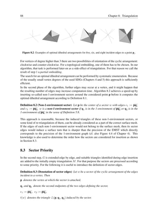
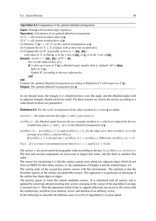


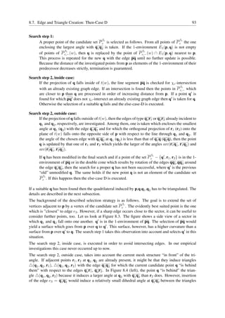
![94 Chapter 8: Triangulation
q’
q
p
q1 , q
2
Figure 8.3: The side view of a configuration in which q′ is selected instead of q.
△(q1 , q2 , r2 ) and △(q1 , q2 , p), cf. Figure 8.4 (right). Therefore it makes sense to consider the quadri-
lateral ✷(p, q1 , q2 , r2 ) to determine the correct triangulation. In order to do this r2 replaces q as the
“new” q.
r2 q
r2
q2
q1 q
q1 , q2 p
p
Figure 8.4: The point q “is behind” the edge q2 r2 (left). The side view (right) shows that it makes sense to consider r2
as new candidate point because the other triangulation of the quadrilateral ✷(p, q1 , q2 , r2 ) with the edge pr2 could yield a
smaller dihedral angle.
8.7.3 Triangulation
The four points p,q1 ,q2 ,q are triangulated according to the min-max triangulation, that is the maxi-
mum angle of the resulting triangles is minimized [HL92].
An alternative approach might be to take that triangulation for which the dihedral angle between the
resulting triangles is greater, and, in the case of equality (which happens in particular if the four points
are co-planar), the min-max triangulation. We did try this possibility, too, and did not recognize a
significant different behavior.
Another alternative is to take the environment of the four vertices in the current surface mesh and
graph into account, with the goal to keep the surrounding mesh smooth. The idea is to maximize the
occurring dihedral angles. The edges of the two possible triangulations of p, q1 , q, q2 are virtually in-
serted into the current surface mesh, and the dihedral angles of the two resulting meshes are estimated
by taking the current dihedral angles at the five edges in the optimal dihedral arrangement of each of
the four vertices. From those of the resulting 10 values which exceed δc the average is taken. Then the
triangulation of p, q1 , q2 , q with the greater average is chosen, and that line segment among pq and
q1 q2 is chosen as candidate edge for insertion which belongs to the selected triangulation.](https://image.slidesharecdn.com/surfacereconstructionrobertmenclphdthesis-130112202114-phpapp01/85/Reconstruction-of-Surfaces-from-Three-Dimensional-Unorganized-Point-Sets-Robert-Mencl-PhD-Thesis-102-320.jpg)
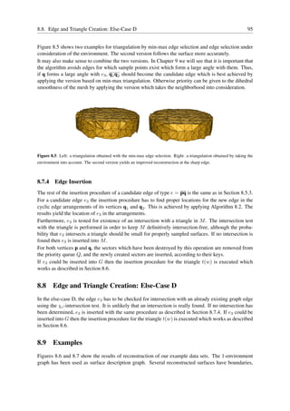
![96 Chapter 8: Triangulation
computation times in minutes and seconds
object # points
DT(P ) clustered 1-EG reconstruction
torus 310 0:01 0:01 0:03
cup 2650 0:11 0:06 0:25
head 1487 0:06 0:03 0:14
skull 698 0:03 0:01 0:05
puppet 695 0:03 0:01 0:07
cap 371 0:02 0:01 0:02
pharaoh 2286 0:10 0:05 0:20
tori 620 0:01 0:02 0:06
Table 8.1: The calculation times of the reconstruction algorithm for the examples on an SGI Octane R10000 at 250 MHz
with 384 MByte of memory.
and the skull additionally has holes which have been properly reconstructed. The parameters used are
listed in the caption of the figures. The calculation times are compiled in Table 8.1. The Delaunay
triangulation DT (P ) has been used as basic data structure for the nearest neighbor queries during the
computation (see Appendix B).
Figure 8.8 shows a sequence of snapshots of the triangulation phase for the clustered β-environment
graph with β = 1 as initial surface description graph for the triangulation.
8.10 Computational Issues
The implementation of the basic data structures of the reconstruction system is based on a library of
template classes. The template classes offer data structures which are used at different locations of
the implementation. In the following section we give a brief survey on these classes. Then the data
structure of the partially ordered surface description graph is described. That data structure supports
the combinatorial requirements of the algorithm, as does the priority queue of sectors to which a
subsection is devoted, too. Finally some aspects of geometric processing, required in particular for the
edge feasibility tests are treated.
8.10.1 A Library of Template Classes
Sorting and containment tests can be carried out with an AVL tree template class. The implementation
of a set class for simple set arithmetics is also based on AVL trees [Wir86].
Whenever sorting is required where the number of objects is not known and where only the first k
elements of a set have to be extracted the heap template class can be chosen. As AVL trees, it has
a run time proportional to O(n log n), but for sorting only subsets of elements heaps are the better
choice.
Of course, template arrays are also part of the library as well as simple list templates, queue templates,
stack templates, and standard string classes.
One interesting part of the library is the integration of so-called hash list classes. Here, the number
of elements to be inserted and the hash function can be adjusted by the programmer and the system
automatically generates an appropriate hash table size. Then, elements can be inserted in this list or
the position of an element can be extracted in constant time.
Space subdivisions for intersection tests, for example, can be realized using several implemented space
subdivision template classes. The basic idea common to all schemes is to subdivide a bounded space](https://image.slidesharecdn.com/surfacereconstructionrobertmenclphdthesis-130112202114-phpapp01/85/Reconstruction-of-Surfaces-from-Three-Dimensional-Unorganized-Point-Sets-Robert-Mencl-PhD-Thesis-104-320.jpg)
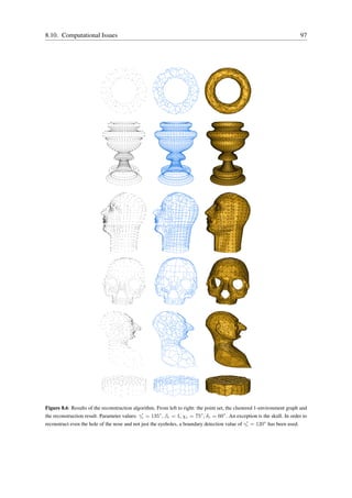
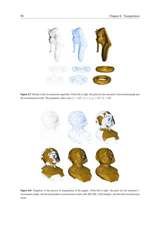


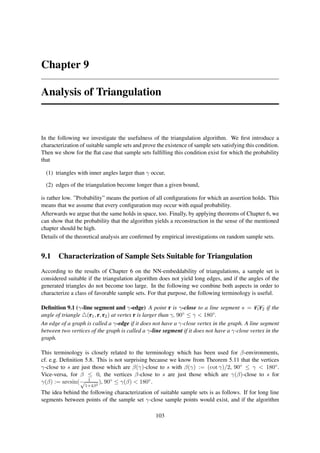
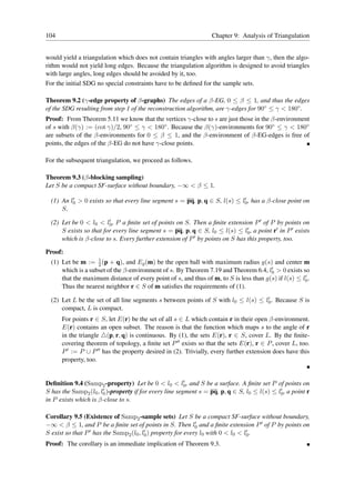


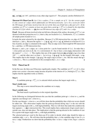
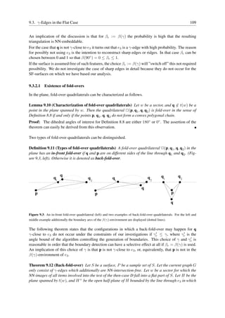
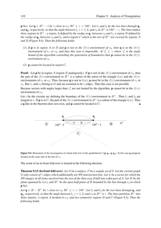
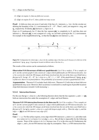
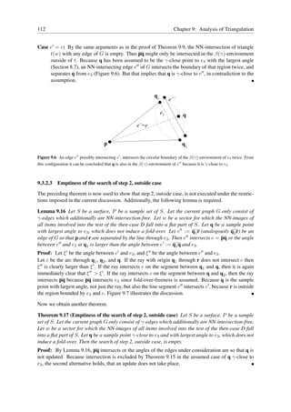
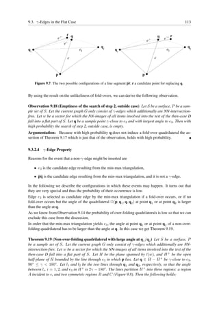
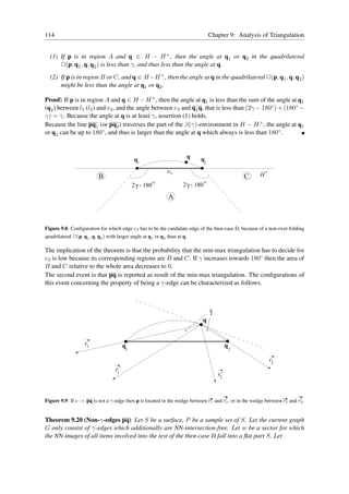
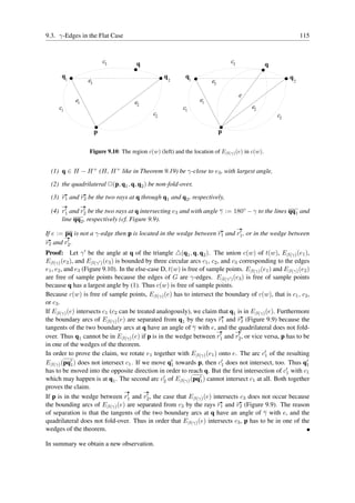

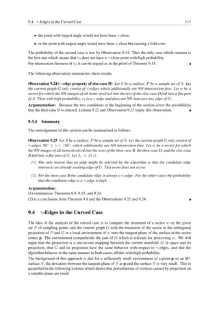
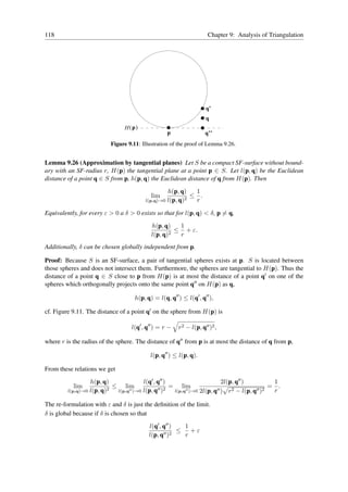
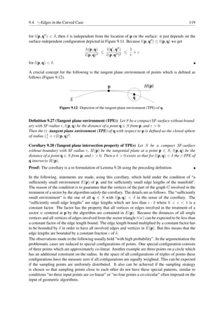
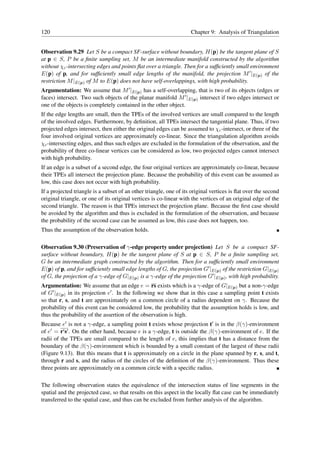
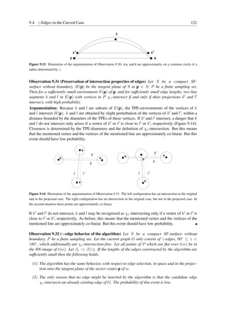
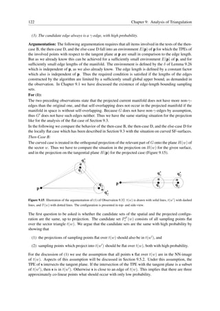
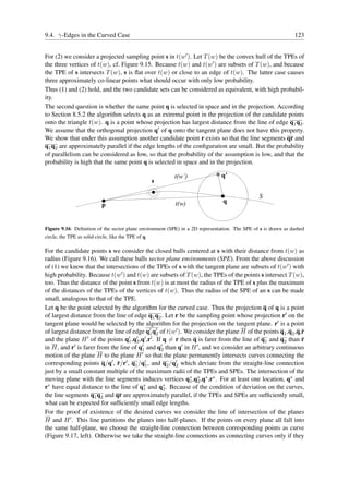

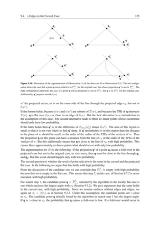
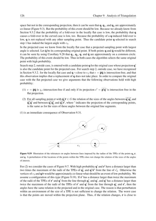
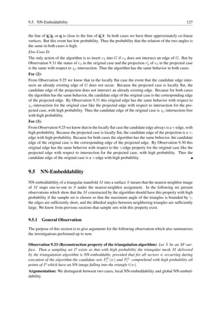
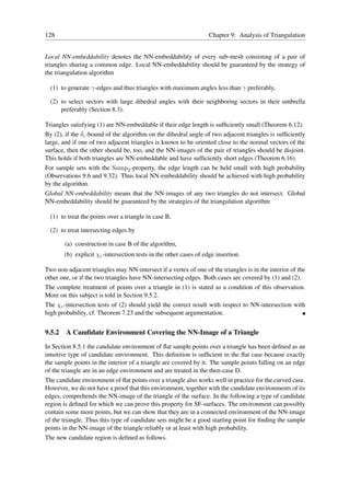
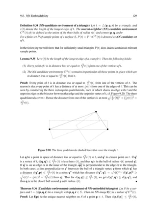

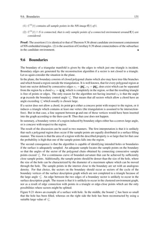
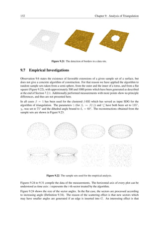
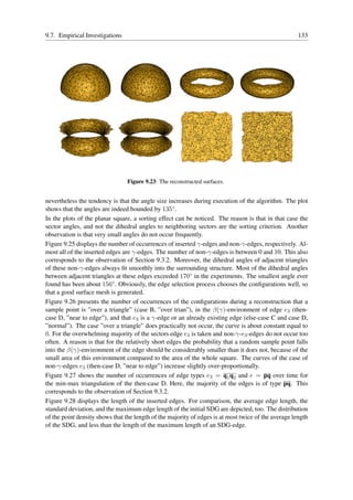
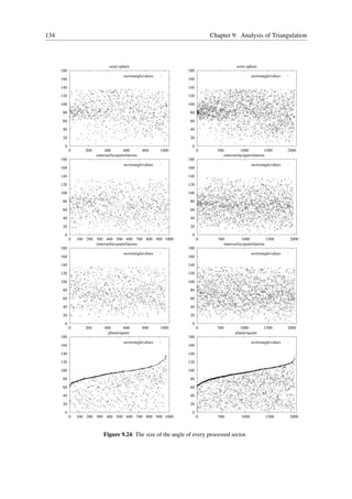
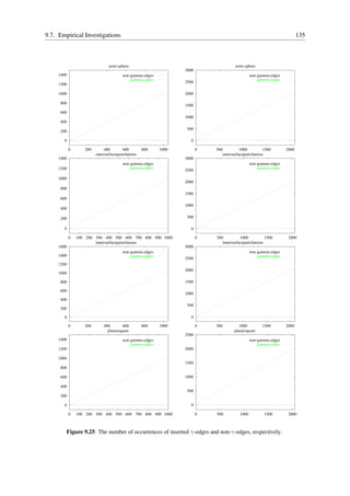
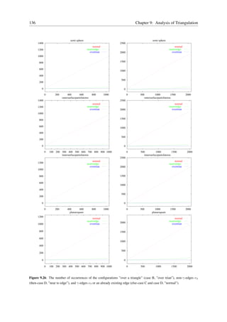
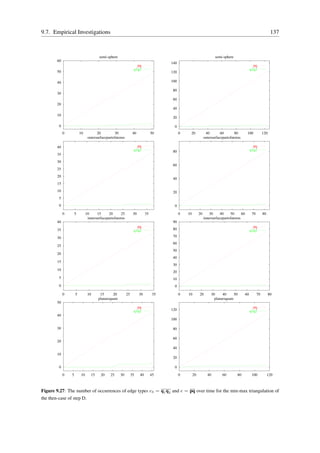
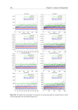
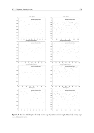
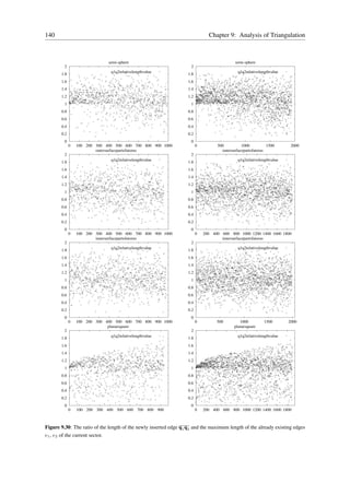
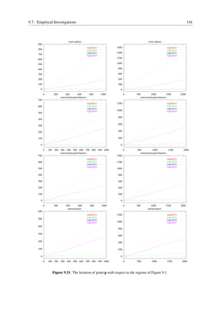
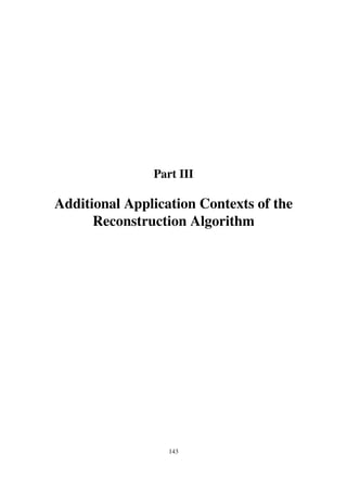


![146 Chapter 10: Interactive (Re-)construction
2. Interactive insertion or deletion of points, and online reconstruction and visualization.
From a computational point of view, the first possibility is easy because the algorithm can be used as
is. It demands some experience of the user with the reconstruction algorithm in order to know how to
set the points to avoid a high number of possibly time-consuming runs of the algorithm.
Online updating after every insertion or deletion in the second case can be performed according to two
main strategies:
1. Recalculation from scratch.
2. Update of the current graph.
From the view of interactivity the first approach is acceptable only if the calculation time is short.
Short calculation times are achieved for small point sets, but become difficult for large sets. Time
can be saved by applying a hierarchical concept. First, just the clustered 1-environment graph (1-
EG) is constructed. If the constructed surface description graph looks sufficiently well, finally the
triangulation is included. That approach is reasonable and acceptable because a good reconstruction
can only be achieved if the earlier graphs already are reasonable. In many cases triangulation from the
surface description is canonical, and no or just little further manipulation of the point set is necessary
in order to get a satisfying result. As we already have seen in Table 8.1 of the previous chapter, the
computation of the clustered 1-environment graph needs just a few seconds if it is computed from
scratch. However, the interactive update is a slightly different task which usually means that only a
small part of the complete graph has to be recomputed. Therefore, even if the point sets get bigger the
update procedure can still have real-time behavior.
Update of the current graph means to provide a data structure which efficiently supports the following
operations:
Vertex insertion:
Given: A set of points and a reconstruction, for example an EG.
Wanted: For an arbitrary additional point, an update of the reconstruction which includes the new
point.
Vertex deletion:
Given: A set of points and a reconstruction, for example an EG.
Wanted: For an arbitrary point of the set, an update of the reconstruction without the selected point.
A simplification is possible by avoiding explicit vertex deletion. The reason is that deletion may
happen only rarely, because slight faults may also be corrected by insertion of further points. If
necessary, vertex deletion can be implemented also on a data structure which just supports insertion
[Ove83]. One approach is to store a sequence of intermediate states of the data structure, and the
sequence of insertions between two consecutive of them. The deletion can be performed by going
back to the state immediately before the insertion of the vertex to be deleted, and process a sequence
of insertions from that point, without inserting the deleted point. This approach works efficiently, if
vertices not too far in the past are eliminated.
More on dynamic data structures for surface description graphs, can be found in Section 10.4.
In the following we give two case studies of interactive modeling from scratch and interactive selective
reconstruction on a given point set.](https://image.slidesharecdn.com/surfacereconstructionrobertmenclphdthesis-130112202114-phpapp01/85/Reconstruction-of-Surfaces-from-Three-Dimensional-Unorganized-Point-Sets-Robert-Mencl-PhD-Thesis-154-320.jpg)
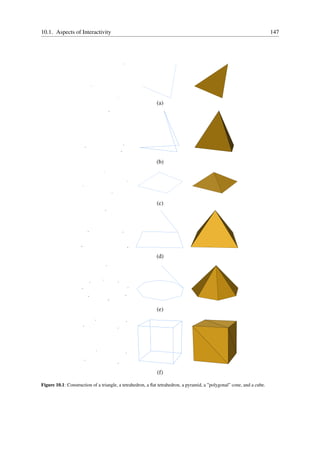
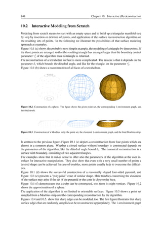
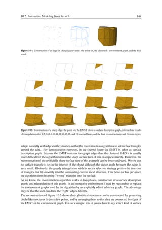
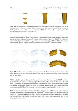
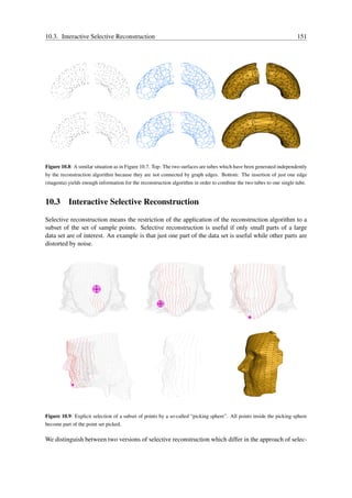
![152 Chapter 10: Interactive (Re-)construction
tion of the subset:
1. Explicit selection of a subset of points which is subject of reconstruction by the surface recon-
struction algorithm.
2. Design of a surface description graph by using points of the given point set, according to one of
the versions of modeling from scratch. From the surface description graph, the manifold can be
constructed by one of the following two possibilities:
(a) Direct usage of the graph for triangulation.
(b) Transformation of the graph into a feasible environment graph under consideration of the
given point set.
An interesting aspect of the first alternative is the method of interactive point selection. Clicking points
individually is tedious for larger point sets. As an alternative we use a selection sphere. The selection
sphere is moved in space, and all those points are selected which have been in the interior of the sphere
during the motion. The radius of the sphere can be changed interactively so that its sensitivity can be
adapted dependent on the details of the region subject to current selection.
Figure 10.10: Top: The point set of the head of a puppet in front and side view. Bottom: The user decides to reconstruct the
nose. The reconstruction region is determined by surrounding the area with six edges, arranged in the shape of a tetrahedron,
which take into consideration the extreme convexity of the nose.
Figure 10.9 shows snapshots of a selection process and the result of reconstruction on the selected
point set. This approach has shown quite useful in particular in combination with a stereoscopic
display and a direct 3D-input by computer-vision-based hand tracking [Blu97, Koh99, SK95].
The background of version 2 (a) is to sketch just a rough wire frame over a subset of points, and the
reconstruction algorithm fills the wire frame in its triangulation phase to a triangular manifold. The
idea behind version 2 (b) is to automatically adapt the sketched graph to the other points of the point
set which is a kind of “projection of the graph to the point set”. This might allow rough sketching,
possibly with long edges, which are then algorithmically refined into edges of an environment graph.](https://image.slidesharecdn.com/surfacereconstructionrobertmenclphdthesis-130112202114-phpapp01/85/Reconstruction-of-Surfaces-from-Three-Dimensional-Unorganized-Point-Sets-Robert-Mencl-PhD-Thesis-160-320.jpg)
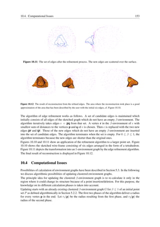

![10.5. Discussion 155
• all points q ∈ P ′ − H which fulfill the relation d(p, q) ≤ max(r2 (p), r2 (p)) +
′
′ ′
max(r2 (q), r2 (q)) with a point p ∈ H and for which r2 (q) = r2 (q).
3’. After the iteration process of step 2’ has taken place, all edges incident to points of H are
deleted. Then, the virtual edges that have been generated in step 2’ are inserted in order of
increasing length using the χ-intersection test. If a new edge χ-intersects an old edge pq that
connects two points p, q ∈ H, then p, q are put onto H, all new already inserted edges are
/
removed, and the iteration process of step 2’ of the update procedure for point insertion is re-
started. This case is very unlikely, since in that case p, q usually would have been close to
points of H and therefore with probability also part of H. If only χ-intersections occur with
new inserted edges of this step 3’ then the update process of the clustered β-environment graph
is complete after all virtual edges have been considered.
10.4.2 Point Deletion
All points p ∈ P with the property d(p, pdel ) ≤ r2 (p) + r2 (pdel ) with respect to the point pdel ∈ P
to be deleted are put onto an initial heap H.
Then, the new point set P ′ is defined by P ′ := P − {pdel } and all edges of the current graph that were
incident to pdel are deleted.
After that, the same update procedure as for point insertion is applied with respect to the different
initial heap H.
10.4.3 Tetrahedrizations for Speed-up
As in Section 5.3, tetrahedrizations are useful for speeding-up the calculation. The following tasks
have to be performed.
The tetrahedrization has to be updated with respect to the manipulated point, that is the point has
to be inserted or deleted. For the Delaunay triangulation, in practice common libraries like the
CGAL [CGA] can be used for that purpose. Unfortunately, up to now there does not seem to ex-
ist any library which handles dynamic deletion of single points from a Delaunay tetrahedrization. For
the hierarchical tetrahedrization insertion does affect just one tetrahedron. Deletion is problematic,
too. A possibility to treat the problem of point deletion is to leave deleted points in the tetrahedriza-
tion and to label them as de-activated. This approach, however, does not work for the supergraph
approach based on Delaunay triangulations mentioned in Section 5.3.
Each time a point is inserted or deleted all points that have ”visited” the modified tetrahedra during
their previous k-nearest neighbor computations have to be re-initialized for this task (Appendix B).
During point insertion, the points with mutually intersecting spheres are identified by processing the
list of points having visited a tetrahedron during a k-nearest-neighbor query, and by comparing their
associated radii. Point deletion is performed analogously. All those points are considered for inter-
secting spheres which have visited the deleted point p in previous nearest neighbor queries.
10.5 Discussion
The surface-oriented approach of our reconstruction algorithm makes it to a useful tool for interac-
tive surface modeling. The surface description graphs provide an efficient computable impression of
the final shape to be expected, and thus are quite useful as control structure of the shape. As sur-
face description graph, the suggested ”automatically” calculated environment graphs, but also graphs
interactively designed or modified by the user can be applied.](https://image.slidesharecdn.com/surfacereconstructionrobertmenclphdthesis-130112202114-phpapp01/85/Reconstruction-of-Surfaces-from-Three-Dimensional-Unorganized-Point-Sets-Robert-Mencl-PhD-Thesis-163-320.jpg)

![Chapter 11
Noise Elimination
A sample set is called noisy if the sample points deviate from the surface by a small, usually random,
distance. Noise in sample sets may be caused by technical properties of the sampling device. If the
sample points deviate considerably from the surface, it might happen that a reconstruction algorithm
that is relying on criteria like the dihedral angle or on neighborhood criteria which assume the surface
to be sufficiently smooth might not longer yield reasonable results.
A powerful method of noise reduction is Laplacian smoothing of second order. This method is origi-
nally defined for distorted vertices of a triangular mesh. In our application, however, we do not have a
mesh before reconstruction. We solve this problem by defining an auxiliary mesh on the given sample
set to which the smoothing operator can be applied for noise reduction.
Figure 11.1: From left to right: The original noisy surface mesh, and the de-noised mesh after 1, 2, and 3 iterations of
Laplacian smoothing of second order. Here, the values α = 0 and β = 0.5 have been chosen. Note, that even after just one
iteration the de-noised mesh has significantly improved.
11.1 Laplacian Smoothing of Second Order
For meshes, the probably up-to-now best smoothing filter is Laplacian smoothing of second or-
der [Tau95, KCVS98, VMM99, Vol98]. Laplacian smoothing of first order considers the set adj(q) of
adjacent vertices of every vertex q of the mesh, and moves it to a new location p which is calculated
by averaging the vertices in adj(q),
1
p := q′ .
n q′ ∈adj(q)
For Laplacian smoothing of second order, basically the same procedure is applied to the difference d
between the new and the original vertex location. This is performed with the slight modification that
at iterative application both the location q at the current level of iteration and the location o of the
vertex in the original mesh are considered by an α-weighted average, as it is done for the differences
157](https://image.slidesharecdn.com/surfacereconstructionrobertmenclphdthesis-130112202114-phpapp01/85/Reconstruction-of-Surfaces-from-Three-Dimensional-Unorganized-Point-Sets-Robert-Mencl-PhD-Thesis-165-320.jpg)
![158 Chapter 11: Noise Elimination
with a weight β, too:
1−β
d := − βb(q) + b(q′ )
|adj(q)| q′ ∈adj(q)
where
b(q) := p − (αo + (1 − α)q).
The result of Laplacian smoothing of second order of a vertex q is the sum of p and d.
The purpose of distance correction by adding d is to reduce the shrinking effect of Laplacian smooth-
ing of first order.
This formula is applied iteratively until a satisfying result is achieved.
The value α weights the influence of the original noisy points. While this is sometimes desired when
existing surface meshes have to be smoothed, the influence of the original points during noise elim-
ination for arbitrary point sets is not favorable. Since the original point positions might have been
generated because of heavy noise the restriction to these positions does not make sense. Therefore, for
this application α = 0 should be chosen. For the other parameter the value β = 0.5 is a good choice
[VMM99].
Figure 11.1 shows an example of an application of Laplacian smoothing of second order to an artifi-
cially noised data set, for α = 0 and β = 0.5.
For mesh smoothing it is of advantage to alternate the application of a surface smoothing operator
like Laplacian smoothing of second order with smoothing by edge swapping [FOG97, DLR90, BS91,
Bro91, Ham97].
Figure 11.2: From left to right: a noisy point set, the auxiliary mesh constructed from it, and the auxiliary mesh smoothed
by alternating the application of Laplacian smoothing of second order and edge swapping.
11.2 Direct Noise Elimination by Auxiliary Meshes
The difficulty in our setting is that no mesh is present with the given sample points. The idea to
cope with that problem is to construct an auxiliary mesh. The auxiliary mesh needs not to be a perfect
reconstruction of the surface, but it should reflect the neighborhood relations between the given sample
points approximately. The basic approach is as follows [VMM99]:](https://image.slidesharecdn.com/surfacereconstructionrobertmenclphdthesis-130112202114-phpapp01/85/Reconstruction-of-Surfaces-from-Three-Dimensional-Unorganized-Point-Sets-Robert-Mencl-PhD-Thesis-166-320.jpg)
![11.3. Discussion 159
1. Calculate a surface description graph (SDG) using the first phase of the reconstruction algorithm
of the previous chapters.
2. If the vertex degrees of the resulting graph are not typical for a surface mesh, augment the set
of adjacent vertices of every vertex by introducing edges up to a suitable number of vertices in
its neighborhood not yet adjacent. In order to take care of variations of the point density, an
adaptive number of nearest neighbors is used, which is estimated by using the length of incident
SDG edges as reference value for the different vertices.
3. Around each vertex a corona of faces is created on base of incident edges like a spanning um-
brella. In this manner for each face one new edge is created, if it does not already exist. These
edges are important for the connectivity of the new mesh.
4. Faces not fulfilling a given mesh quality measure are removed. A quality measure introduced
by Bank and Smith [BS97] is used for that purpose.
5. Remove triangles so that at most two triangles are incident to every edge in order to make edge
swapping applicable, under preservation of pairs of triangles with large dihedral angles. All
edges which do not have at least one incident face are removed.
Step 5 is necessary because the set of triangles generated in the previous steps may be non-manifold.
Figure 11.3: Reconstruction based on the noise-reduced set of points shown at the left.
Figure 11.2 shows a distorted sampling set of a bone, the derived auxiliary mesh, and the result of
smoothing of that mesh by an alternating application of Laplacian smoothing of second order and
edge swapping. Figure 11.3 depicts the noise-reduced point set and the reconstruction of the bone
obtained by our reconstruction algorithm from this point set.
11.3 Discussion
The approach of using an auxiliary mesh for smoothing of noisy point sets sampled from a smooth
surface has turned out to be useful in practical examples. A topic of further research might be to extend
the theoretical investigations of this thesis which assume the sampling points being on the surface, to
sampling points only close to the surface. A triangular mesh with those noisy sampling points as
vertices might be considered as reconstruction of the given surface, if it maps one-to-one under the
NN-image to a non-overlapping mesh on the surface.](https://image.slidesharecdn.com/surfacereconstructionrobertmenclphdthesis-130112202114-phpapp01/85/Reconstruction-of-Surfaces-from-Three-Dimensional-Unorganized-Point-Sets-Robert-Mencl-PhD-Thesis-167-320.jpg)


![164 Chapter 12: Future Developments and Conclusion
which are likely to avoid unfavorable situations. For example, a well-suited sampling strategy is to
choose the sampling points as vertices of a quadrilateral mesh whose faces are moderately distorted
squares. Additionally, our empirical investigations have shown that the unfavorable configurations
are only unfavorable for the mathematical analysis and not for the reconstruction in practice. In all
of our examples, the accuracy of the reconstruction in those cases is not influenced. Obviously, the
triangulation criteria always choose surface triangles with a good approximation quality. This leads
to the assumption that the triangles “inherit” their surface approximation quality from the surrounding
triangles and it can be expected that mathematical arguments for this property can be found.
The analysis has been performed only for smooth surfaces, represented by so-called SF-surfaces S.
The mathematical treatment of sharp edges is a problem for further research. An approach for a
solution could be the consideration of singular surface points and what kind of sampling in those areas
is needed and then extend this principle to surface ridges.
We have restricted our discussion to the existence of suitable sampling sets, not having the goal of
sampling sets of minimum cardinality. A step in this direction would be to take into consideration the
maximum possible SF-radius at every point, not just a constant radius r for the whole surface which
bounds the occurring SF-radii from below. Our investigations can be generalized in the direction by
replacing the constant r with a function r : S → I + for which r(p) is at most equal to the maximum
R
SF-radius at p.
A further idea is to get independent from the quality of the sampling by using feature recognition in
the surface description graph [MM98a, Mai98] if the graph itself does not contain enough surface in-
formation. The feature knowledge could be used in order to modify the graph so that the triangulation
algorithm can generate a correct surface mesh even if the sampling was not sufficient. In order to
improve flexibility in this approach, the recognition capabilities can be formulated in rules that can be
also changed during run-time and interpreted by a rule evaluation system [Hei98].
As these remarks show, much has been achieved, but some interesting questions remain for future
research. In conclusion, however, we believe that the approach presented in this thesis is a particular
flexible and precise alternative to other approaches. It is well-suited for practical applications, even on
non-dense data sets, and it allows useful assertions on the requirements of sampling.](https://image.slidesharecdn.com/surfacereconstructionrobertmenclphdthesis-130112202114-phpapp01/85/Reconstruction-of-Surfaces-from-Three-Dimensional-Unorganized-Point-Sets-Robert-Mencl-PhD-Thesis-172-320.jpg)


![Appendix A
Implementation
The reconstruction algorithm has been implemented in C++ using the toolkits Tcl/Tk [Ous94], Tix
[Lam93] and OpenInventor [Wer94]. These toolkits were taken because of their effectiveness in the
design of graphical user interfaces as well as in the development of complex geometry viewers.
Figure A.1: A screenshot of the reconstruction system R EC E YE. Left: the control panel. Right: the geometry viewer with
an intermediate reconstruction.
The graphical user interface of the reconstruction system R EC E YE is separated into a control panel
and a geometry viewer window, cf. Figure A.1.
The control panel contains three sub-windows, the Reconstruction Control, Interaction Settings, and
the Execution Log window.
The Reconstruction Control contains the basic buttons for the standard usage of the system. With Load
Points the point set specified by the current file name <pointfile>.pts is loaded. The program
167](https://image.slidesharecdn.com/surfacereconstructionrobertmenclphdthesis-130112202114-phpapp01/85/Reconstruction-of-Surfaces-from-Three-Dimensional-Unorganized-Point-Sets-Robert-Mencl-PhD-Thesis-175-320.jpg)
![168 Appendix A: Implementation
expects an already existing tetrahedron file <pointfile>.tl which contains the Delaunay tetra-
hedrization of the point file. The first line of the file will be skipped, all other subsequent lines contain
the point indices of the tetrahedra of the Delaunay tetrahedrization. For the Delaunay tetrahedrization
the program D ETRI of M¨ cke [M¨ c93b, M¨ c93a] can be used. The other buttons Cl. 1-EG (Clustered
u u u
1-EG) and Triangulation belong to the specific phases of the reconstruction algorithm. The (interme-
diate) results are saved using the geomview file format into the files <pointfile>.sdg.geom, for
the graph, and <pointfile>.s.geom for the triangular mesh. The Point File and Exit buttons are
self-explaining.
Figure A.2: The sub-menues for the interaction settings menues Edit and Inspect.
Figure A.3: The sub-menues for the interaction settings menues Graphs and Parameters/Options.
In the Interaction Settings the relevant data for the user interaction can be set. The menues are subdi-
vided into 5 different categories: View, Edit, Inspect, Graphs, and Parameters/Options. An overview
of these menues can be found in Figures A.1, A.2, and A.3.
In the following we give a short description of these five menues.
• View:
– Viewer Settings: Here, the Reconstruction Viewer window, the Trace Mode for the recon-
struction and stereo viewing can be switched on/off.
– Stereo Settings: The eye distance offset of the stereo mode can be changed here.
– Geometry Display: The size of the points in order to simplify picking can be increased.](https://image.slidesharecdn.com/surfacereconstructionrobertmenclphdthesis-130112202114-phpapp01/85/Reconstruction-of-Surfaces-from-Three-Dimensional-Unorganized-Point-Sets-Robert-Mencl-PhD-Thesis-176-320.jpg)
![169
– Set Default Window Geometry: The default window geometry for both windows (Rec-
Eye), the control window alone (RecEye Menu), or just the reconstruction viewer window
(RecEye Viewer/Editor) can be set.
• Edit:
– Picking Device: The user can switch between the standard Mouse, the hand gesture pick-
ing (GePi Hand Gesture), and 3D movement of a picking sphere with simple mouse in-
teraction as it is supported by OpenInventor [Wer94]. Picking with the simple mouse is
performed in the picking mode of OpenInventor by first clicking onto the “arrow” in the
upper right of reconstruction viewer window and then clicking on the points. In order to
being able to turn the object in the reconstruction viewer window, the “hand symbol” in
the upper right window has to be clicked. The hand gesture picking also moves a picking
sphere through the point set. The set of points that is inside the picking sphere is picked.
This hand gesture picking approach uses the library G E P I [Blu97] based on the hand ges-
ture recognition system Z YKLOP [Koh99, SK95]. The description of the control of this
system can be found in [Blu97].
– Editing Commands: Pairs of points can be inserted as an edge (Connect Points) or their
connecting edge can be deleted (Disconnect Points). Point triplets induce the deletion
(Delete Triangle) and insertion (Build Triangle) of triangles. For the connection/discon-
nection of points and for the triangle deletion/insertion exactly two or three points, respec-
tively, have to be picked.
– Picked Objects: The picked points as well as their complement can be saved into the file
<pointfile>.[un]picked.
• Inspect:
– Inspection Mode: The Step-by-Step mode of the triangulation can be activated and each
time a Step Forward by inserting one triangle after another, the reconstruction process can
be investigated. In the Data Inspection Mode some additional information is printed which
describes the internal computations for various modules of the system.
– Inspect Objects: In this section the various objects which became important during the
development of the reconstruction algorithm can be investigated.
• Graphs:
– Compute Different Graphs: The EMST, the clustered β-EGs with β = 1, β = 0.5, β = 0
and their corresponding non-clustered β-EGs can be computed. All computed edges are
added to the current graph.
– Graph Modifications Related to Locally-Restricted Reconstruction: The “graph projec-
tion approach” of Chapter 10 for locally-restricted reconstruction can be applied here.
– General Graph Modification: With the button Remove All Graph Edges, the current graph
can be reset to the empty graph.
• Parameters/Options:
– Algorithm Parameters: The parameters of the triangulation algorithm can be changed here.
– Reconstruction Parameters: The number of faces to be inserted in one triangulation step
can be modified here. If the value is 0 then the complete mesh is generated.
– Optional Triangulation Snapshots: Four different values for the number of faces,
where the current triangulation mesh has to be saved into a snapshot file
<pointfile>.shot#.s.geom in the geomview file format.](https://image.slidesharecdn.com/surfacereconstructionrobertmenclphdthesis-130112202114-phpapp01/85/Reconstruction-of-Surfaces-from-Three-Dimensional-Unorganized-Point-Sets-Robert-Mencl-PhD-Thesis-177-320.jpg)

![Appendix B
Efficient and Flexible Nearest Neighbor Queries
Because of their occurrence in many applications, the efficient solution of nearest-neighbor problems
has found particular interest in computational geometry in the past. Two main streams of approaches
may be distinguished. One of them is centered around the concept of Voronoi-diagrams [PS85] the
other one on more arbitrary spatial decompositions [AM91]. For solutions of the first stream, effi-
cient worst case time bounds can often be proved, whereas for second type of approaches, the worst
case behavior often is bad but they behave quite well in practice. Often, the heuristics are easier
to implement than the more sophisticated Voronoi-diagram-based approaches. The solution of the
k-nearest-neighbor problem falls in the second category.
In previous work on heuristic solutions of nearest neighbor problems [CK92, AMN+ 94], regular space
subdivisions play an important role. These subdivisions perform well on uniformly distributed data,
but are somewhat less suited for data sets of strongly varying density. Triangulations, on the other
hand, are an irregular data structure which adapts easily to all kinds of data distributions.
B.1 k-Nearest-Neighbor Search
The aim of the following is, as a result of the above considerations, to present an algorithm for solving
the k-nearest-neighbors problem by taking advantage of a previously computed triangulation. A d-
dimensional triangulation is defined as follows.
Definition B.1 (d-dimensional triangulation) Let A be a real-affine space of dimension d with met-
ric d(·, ·). An m-simplex s is the convex hull of m + 1 points, called vertices, which are not contained
in a (m − 1)-dimensional subspace. A subsimplex of s is the convex hull of a proper subset of the
vertices of s. A (d−1)-subsimplex of a d-simplex is called a facet. Two d-simplices are called incident
if one of them is a subsimplex of the other. Two d-simplices are called adjacent if they have d vertices
in common and their intersection is a facet.
We define the distance of a simplex s from a point p as
d(s, p) := min d(q, p) .
q ∈s
Let the point set P = {p1 , . . . , pn } ⊂ A not be contained in a proper subspace of A. A triangulation
T of P is a tesselation of the convex hull of P into d-simplices whose vertices are in P . We denote the
subsimplices of all d-simplices of T collectively as the subsimplices of T . In particular, the points in
P are the 0-subsimplices of T .
The basic version of the problem we are treating is defined as follows.
171](https://image.slidesharecdn.com/surfacereconstructionrobertmenclphdthesis-130112202114-phpapp01/85/Reconstruction-of-Surfaces-from-Three-Dimensional-Unorganized-Point-Sets-Robert-Mencl-PhD-Thesis-179-320.jpg)
![172 Appendix B: Efficient and Flexible Nearest Neighbor Queries
Definition B.2 (k-nearest-neighbors query)
Input: A vertex pi of a d-dimensional simplicial decomposition T .
Output: The k-nearest vertex to pi in T .
Our algorithm for that problem can process multivariate data, as it functions in spaces of arbitrary finite
dimension. Furthermore, it does not assume a particular metric. Many triangulation-based algorithms
will work only with triangulations that possess certain properties, such as Delaunay triangulations.
Our algorithm makes no such requisites. Thus, it can operate on any triangulation that another module
has ‘left behind.’ In determining the k nearest neighbors, our algorithm explores only a part of the
triangulation. While this part contains more vertices than just the k nearest ones, it is in general
considerably smaller than the complete triangulation. The neighbor points are reported in order of
increasing distance from the query point. In some applications, this order presents useful additional
information. Implementation of the algorithm is straightforward. Apart from distance computations
and the triangulation, only standard operations and data structures are needed.
With only minor modifications, the algorithm becomes applicable to slightly different types of queries.
Thus, it is easy to find the data points lying within a certain radius from the query point. Not only
vertices of the triangulation, but arbitrary points in the respective space can be used as query points.
A query can be suspended after a certain number of neighbors have been determined, to be resumed
later if further neighbors are needed. This is particularly useful for interactive graphical techniques
where additional demand for neighborhood information arises as a result of feedback from the user.
The basic concept of our algorithm [WM96] is a ball which is centered at the query point pi and
whose radius increases continuously. As the ball expands, it encounters the vertices of T in order of
increasing distance from pi . Our algorithm registers not only the vertices, but also the d-simplices of
T in the order in which the ball encounters them. To this end, an appropriate subset of the d-simplices
and vertices is stored in a heap, which is sorted by distance from the query point. The element closest
to pi is found at the top of the heap.
The expanding ball will, in general, encounter several d-simplices and/or vertices simultaneously. The
algorithm, on the other hand, processes these elements one after another. At any given time during
the expansion process, we call a d-simplex or vertex of T intersecting if the algorithm has determined
that it intersects the ball. All other d-simplices and vertices are called non-intersecting, even if they
do intersect the ball. The term closest is used with respect to distance from the query point.
Lemma B.3 Let pi be contained in at least one intersecting d-simplex. Then one of the closest non-
intersecting d-simplices is adjacent to (i.e., shares a facet with) an intersecting d-simplex.
Proof: Let t be a closest non-intersecting d-simplex, and let q be the point of t closest to pi . Since
T covers a convex volume, it must cover the line segment pi q. By choice of t and q, it is clear that
each interior point of pi q is contained in some intersecting d-simplex. Since we consider closed d-
simplices, q is also contained in an intersecting d-simplex, say, t′ . (If the line segment has no interior
points, then q = pi is contained in an intersecting d-simplex by hypothesis.) Now consider two
interior points, p and p′ , of t and t′ , respectively. We choose these points sufficiently close to q that
the line segment p′ p is covered by d-simplices containing q. If necessary, we perturb the points such
that p′ p does not intersect any subsimplex of T of dimension less than d − 1. At some point between
p′ and p, the line segment must pass from an intersecting into a non-intersecting d-simplex. This point
is interior to a facet f, which is shared by the two d-simplices. Since the non-intersecting d-simplex
contains q, it is a closest non-intersecting d-simplex.
The algorithm starts by inserting one d-simplex incident on pi into the empty heap. It then keeps
processing simplices from the top of the heap until it has found the k nearest neighbors. If the simplex](https://image.slidesharecdn.com/surfacereconstructionrobertmenclphdthesis-130112202114-phpapp01/85/Reconstruction-of-Surfaces-from-Three-Dimensional-Unorganized-Point-Sets-Robert-Mencl-PhD-Thesis-180-320.jpg)

![174 Appendix B: Efficient and Flexible Nearest Neighbor Queries
the case k < n − 1, we simply note that the algorithm runs in exactly the same way as for n − 1
neighbors, but stops after the k nearest neighbors have been found.
pi pi
Figure B.1: Two phases of the algorithm as the expanding ball encounters a vertex and, simultaneously, three triangles.
Figure B.1 shows two snapshots of the algorithm working on a planar triangulation. The intersecting
triangles and vertices are drawn in white and black, respectively. The triangles and vertices in the heap
are drawn in gray. In the left diagram, the algorithm has just deleted a vertex from the heap. In the
right diagram, it has also processed the triangles that are incident on this vertex.
Concerning the analysis of the time complexity of the algorithm, we assume that the data structure of
the triangulation allows us to carry out the following operations:
• Given a vertex, find an incident d-simplex in constant time.
• Given a d-simplex, find its vertices in time O(d).
• Given a d-simplex, find the d + 1 adjacent d-simplices in time O(d).
One elementary step in Algorithm B.1 is the distance computation between a d-simplex and the query
point. The time complexity of this step depends on the dimension and on the metric being used. In
d-dimensional space, it takes time proportional to d to determine the Euclidean distance between two
points alone. In the following, we let δ denote the worst-case complexity of distance computations,
both between two points and between a point and a d-simplex.
Let |T | denote the number of d-simplices in T , and let |H| be the number of simplices contained in
H. We note that n ∈ O(|T |). In the planar case, we also have |T | ∈ O(n). In 3-dimensional space,
triangulations with |T | ∈ O(n) exist and can be constructed in O(n log n) time (cf. [EPW90]).
To analyze the time complexity of the overall algorithm, let us first look at the time spent on heap
operations. An insertion or deletion takes O(log |H|) time. Each vertex and each d-simplex is inserted
into, and, likewise, deleted from, the heap at most once. Therefore, both the number of heap operations
and the heap size are bounded by O(|T |). The total time for all heap operations is O(|T | log |T |) in
the worst case. Distance computations are carried out only for those simplices which are inserted into
the heap, and only once per simplex. Therefore, the total time for distance computations is bounded
by O(δ |T |).](https://image.slidesharecdn.com/surfacereconstructionrobertmenclphdthesis-130112202114-phpapp01/85/Reconstruction-of-Surfaces-from-Three-Dimensional-Unorganized-Point-Sets-Robert-Mencl-PhD-Thesis-182-320.jpg)

![B.2. An Object-Oriented Framework for Flexible and Adaptive Nearest Neighbor Queries 177
The cost for searching first k and then the next ℓ neighbors is the same as for searching k + ℓ neighbors
in a single query. Some information must be saved in order to resume a query. This comprises the
heap H, the flags, and the number k of previously found neighbors. We call this information nearest
neighbor query iterator (NNQ iterator).
It is also possible to run queries in a concurrent manner, e.g., find ki neighbors of pi , then kj neigh-
bors of pj , then another ℓi neighbors of pi , etc. Multiple suspended queries require a nearest neigh-
bor iterator for each query point. Suppose that concurrent queries are carried out for all n vertices,
then the space requirement for the flags is proportional to n |T |. However, if the average number of
neighbors computed per vertex is small, most of the flags will never be used. Storage space can be
reduced if we replace the flags by a hash table. Instead of setting a flag, we insert a pair of the form
(query point , ‘flagged’ simplex) into the table. By the very nature of concurrent queries, the required
number of neighbors in a single query is not known in advance. Thus, it may be impossible to make an
appropriate choice for the size of the hash table, which has a strong influence on the table’s efficiency.
As an alternative, we can substitute a sorted tree (e.g., AVL or SBB tree, cf. [Wir86]) for each heap,
i.e., one per query. We insert s′ into the tree if it is not contained in the tree and was not processed
before s. Containment in the tree can be tested efficiently. Simplices are processed in order of in-
creasing distance from the query point. Therefore, if s′ is strictly closer than s, it has been processed
before, and if s′ is strictly further than s, it has not been processed before. Equidistant simplices that
have been processed are stored in an auxiliary tree, and can be found there. A simplex is inserted into
the auxiliary tree as soon as it is processed. The auxiliary tree is cleared when the intersecting sphere
expands, i.e., when a simplex of greater distance is processed.
B.2 An Object-Oriented Framework for Flexible and Adaptive Nearest
Neighbor Queries
Usually, nearest neighbor queries are only considered from the algorithmical point of view and not
from the implementation view. Since the nearest neighbor task is a frequent problem in many ap-
plications we show how the implementation can be done with respect to our algorithmical solution.
The reason for this is, that our approach is so general that it allows an easy-to-follow object-oriented
approach that simplifies the implementation. Another advantage is that this framework can be ad-
justed to several similar tasks of nearest neighbor queries, for example, if using other types of spatial
subdivisions besides tetrahedrizations/triangulations.
In the following we describe the basic approach how the implementation can be done. In our ex-
ample we restrict the types of query objects to single points and the type of spatial subdivisions to
tetrahedrizations as examined in theory for the k nearest neighbor search in the previous section. But
extension to arbitrary types of objects (polyhedrons) is straightforward. The only thing that has to be
considered is an appropriate distance function for the kind of object that is used as query object and the
surrounding polyhedral cells. The already reported neighbors are stored in a list that is associated with
the query point so that concurrent queries that are carried out from different positions of the program
do not repeat unnecessary computations. This means, that if the number of needed neighbors is below
the number of already computed neighbors, only the elements of the neighbor list of a query point
have to be iterated in order to complete the query task. This holds as long as the tetrahedrization is not
modified. But even if this is the case, local modifications mean only local influence on the neighbor
structure for the points in the modified regions, so that an update can be established efficiently by only
updating the points that have already “traversed” the modified region with their expanding ball.
For better understanding of the implementation be have chosen a simplified and more readable version
of C++ – like program code. This code should be comprehensible for everyone who is familiar with
object-oriented concepts in an arbitrary programming language.](https://image.slidesharecdn.com/surfacereconstructionrobertmenclphdthesis-130112202114-phpapp01/85/Reconstruction-of-Surfaces-from-Three-Dimensional-Unorganized-Point-Sets-Robert-Mencl-PhD-Thesis-185-320.jpg)
![178 Appendix B: Efficient and Flexible Nearest Neighbor Queries
Simplex
// Boolean functions:
updateNeighborList();
updateNeighborsInTree(PointPtr);
Point Tetrahedron AnySimplexClass
...
// List of neighbor points:
neighborList;
// Sorting tree of simplices
simplexNeighborTree;
// Boolean functions: // Boolean function: // Boolean functions:
updateNeighborList(); updateNeighborList();
updateNeighborsInTree(PointPtr); updateNeighborsInTree(PointPtr); updateNeighborsInTree(PointPtr);
Figure B.4: The UML class diagram of the nearest neighbor query implementation.
We assume an arbitrary tetrahedrization is already given and use this information within the nearest
neighbor query algorithm.
The UML class diagram (unified modeling language) [BRJ99] of our implementation is shown in
Figure B.4. In our application we need a Point class and a Tetrahedron class that are both derived
from the class Simplex. Since this concept is extensible to any type of nearest neighbor queries
for each kind of simplex, there also can be implemented a nearest neighbor query for an arbitrary
simplex class which is denoted in the diagram as AnySimplexClass. The most important parts of the
diagram are the virtual functions updateNeighborList() and updateNeighborsInTree() of
class Simplex that are overloaded in each implementation inside the class Point or Tetrahedron.
These are the main functions needed in the realization of a k-nearest-neighbor query algorithm. As we
see in the diagram the function updateNeighborList() is only implemented for the Point class,
since we restrict our queries to points. But as mentioned before, arbitrary queries for other object types
than points would be possible, too. For example, if one would like to implement a nearest neighbor
query for tetrahedrons, it is sufficient to implement the function updateNeighborList() for the
Tetrahedron class.
In the following we describe how the concept of the UML class diagram can be used in order to
implement nearest neighbor queries for points. Class NnqIterator delivers the frame work for
an instantiation of a nearest neighbor query iterator for a query point q, cf. Figure B.5. It consists
of a pointer to a point that describes the query object, and a list iterator that iterates on the list of
nearest neighbors already found. This neighborList is associated with each query point. In the
beginning the neighborList is empty before a query has taken place for the query point. With
the reset() function of NnqIterator the iterator can be set to the beginning of a neighbor query
which responds to the situation where the query ball has radius zero. In order to get a nearest neighbor
the get() function of NnqIterator is then called. Then the next point that is delivered is the
nearest neighbor of the query. Each time the get() function is called a new neighbor is computed
and appended to the neighborList that is associated with the query point q. But first it is checked](https://image.slidesharecdn.com/surfacereconstructionrobertmenclphdthesis-130112202114-phpapp01/85/Reconstruction-of-Surfaces-from-Three-Dimensional-Unorganized-Point-Sets-Robert-Mencl-PhD-Thesis-186-320.jpg)


![Bibliography
[AB98] N. Amenta and M. Bern. Surface reconstruction by voronoi filtering. In 14th ACM
Symposium on Computational Geometry, pages 39–48, 1998.
[ABK98] N. Amenta, M. Bern, and M. Kamvysselis. A new voronoi–based surface reconstruction
algorithm. Computer Graphics, pages 415–421, 1998. Proceedings of SIGGRAPH ’98.
[AC99] N. Amenta and S. Choi. One-pass Delaunay filtering for homeomorphic 3D surface
reconstruction. Technical Report TR99-08, University of Texas, Austin, 1999.
[ACDL00] N. Amenta, S. Choi, T.K. Dey, and N. Leekha. A simple algorithm for homeomorphic
surface reconstruction. In Proceedings of 16th ACM Sympos. Comput. Geom., July 2000.
[ACK01] N. Amenta, S. Choi, and R. K. Kolluri. The power crust, unions of balls, and the medial
axis transform. Computational Geometry: Theory and Applications, 19(2-3):127–153,
2001.
[AGJ00] U. Adamy, J. Giesen, and M. John. New techniques for topologically correct surface re-
construction. In Proceedings of IEEE Visualization 2000. IEEE Computer Society Press,
2000.
[AGJ01] U. Adamy, J. Giesen, and M. John. Surface reconstruction using umbrella filters. Com-
putational Geometry: Theory and Applications, 2001.
[AM91] S. Abramowski and H. M¨ ller. Geometrisches Modellieren. BI–Wiss.–Verl., 1991. Bd.
u
75.
[AMN+ 94] S. Arya, D.M. Mount, N.S. Netanyahu, R. Silverman, and A. Wu. An optimal algorithm
for approximate nearest–neighbour searching. In Proceedings 11th Annual Symposium
on Discrete Algorithms, pages 573–582, 1994.
[AS96] M.-E. Algorri and F. Schmitt. Surface reconstruction from unstructured 3D data. Com-
puter Graphics Forum, 15(1):47–60, 1996.
[AS00] M. Attene and M. Spagnuolo. Automatic surface reconstruction from point sets in space.
Computer Graphics Forum, 19(3), 2000. Proceedings of EUROGRAPHICS 2000.
[Att97] D. Attali. r-regular shape reconstruction from unorganized points. In ACM Symposium
on Computational Geometry, pages 248–253, 1997. Nice, France.
[Baa95] A. Baader. Ein Umwelterfassungssystem f¨ r multisensorielle Montageroboter. PhD the-
u
sis, Universit¨ t der Bundeswehr, Munich, Germany, 1995. Fortschrittberichte, VDI Reihe
a
8 Nr. 486, ISBN 3-18-3 48608 - 3, ISSN 0178-9546.
183](https://image.slidesharecdn.com/surfacereconstructionrobertmenclphdthesis-130112202114-phpapp01/85/Reconstruction-of-Surfaces-from-Three-Dimensional-Unorganized-Point-Sets-Robert-Mencl-PhD-Thesis-191-320.jpg)
![184 BIBLIOGRAPHY
[BB97] F. Bernardini and C. Bajaj. Sampling and reconstructing manifolds using alpha-shapes.
In Proc. of the Ninth Canadian Conference on Computational Geometry, pages 193–198,
August 1997. Also available as Technical Report CSD-97-013, Department of Computer
Sciences, Purdue University.
[BBCS97] F. Bernardini, C. Bajaj, J. Chen, and D.R. Schikore. Automatic reconstruction of 3D
CAD models from digital scans., 1997. Technical Report CSD-97-012, Department of
Computer Sciences, Purdue University.
[BBX95] C.L. Bajaj, F. Bernardini, and G. Xu. Automatic reconstruction of surfaces and scalar
fields from 3D scans. Computer Graphics Proceedings, SIGGRAPH ’95, Annual Confer-
ence Series, pages 109–118, 1995.
[BBX97] C. Bajaj, F. Bernardini, and G. Xu. Reconstructing surfaces and functions on surfaces
from unorganized 3D data. Algorithmica, 19:243–261, 1997.
[Ben74] C. Bender. Bestimmung der gr¨ ssten Anzahl gleicher Kugeln welche sich auf eine Kugel
o
¨
von demselben Radius, wie die ubrigen, auflegen lassen. Archiv Math. Physik (Grunert),
56:302–306, 1874.
[Ber63] C. Berge. Topological Spaces. Oliver & Boyd Ltd., Edinburgh and London, 1963.
[Ber96] F. Bernardini. Automatic Reconstruction of CAD Models and Properties from Digital
Scans. PhD thesis, Department of Computer Science, Purdue University, 1996.
[BH93] A. Baader and G. Hirzinger. Three–dimensional surface reconstruction based on a self–
organizing feature map. In Proc. 6th Int. Conf. Advan. Robotics, pages 273–278, 1993.
Tokyo.
[BH94] A. Baader and G. Hirzinger. A self–organizing algorithm for multisensory surface recon-
struction. In International Conf. on Robotics and Intelligent Systems IROS ’94, Septem-
ber 1994. Munich, Germany.
[BJMT99] F. Bernardini, C. Silva J. Mittleman, H. Rushmeier, and G. Taubin. The ball-pivoting
algorithm for surface reconstruction. IEEE Transactions on Visualization and Computer
Graphics, 5(4), 1999.
[Blu97] S. Blumenthal. Moderne Methoden der Mensch-Maschine-Interaktion im Geometrischen
Modellieren. Master’s thesis, Informatik VII (Computer Graphics), University of Dort-
mund, Germany, 1997.
[Boe52] A. H. Boerdijk. Some remarks concerning close-packing of equal size. Philips Res. Rep.,
7:303–313, 1952.
[Boi84] J.-D. Boissonnat. Geometric structures for three-dimensional shape representation. ACM
Transactions on Graphics, 3(4):266–286, October 1984.
[Bor26] O. Bor˚ vka. O jist´ m probl´ mu minim´ lním.
u e e a Pr´ ce moravsk´ pˇ írodovˇ deck´
a e r e e
spoleˇ nosti, 3:37–58, 1926. in Czech.
c
[BRJ99] G. Booch, J. Rumbaugh, and I. Jacobson. The Unified Modeling Language User Guide.
Addison-Wesley, 1999.](https://image.slidesharecdn.com/surfacereconstructionrobertmenclphdthesis-130112202114-phpapp01/85/Reconstruction-of-Surfaces-from-Three-Dimensional-Unorganized-Point-Sets-Robert-Mencl-PhD-Thesis-192-320.jpg)
![BIBLIOGRAPHY 185
[Bro91] J.L. Brown. Vertex based data dependent triangulations. Computer Aided Geometric
Design, 8:239–251, 1991.
[BS87] I.A. Bronstein and K.A. Semendjajew. Taschenbuch der Mathematik. Verlag Harri
Deutsch, 1987.
[BS91] G. Baszenski and L.L. Schumaker. Use of simulated annealing to construct triangular
facet surfaces. In Curves and Surfaces, pages 27–32. Academic Press, Boston, 1991.
[BS96] C. Bajaj and D. Schikore. Error-bounded reduction of triangle meshes with multivariate
data. In Proceedings of SPIE Symposium on Visual Data Exploration and Analysis III,
pages 34–45, January 1996. SPIE.
[BS97] R.E. Bank and R.K. Smith. Mesh smoothing using a posterior error estimation. SIAM
Journal on Numerical Analysis, 1997.
[BTG95] E. Bittar, N. Tsingos, and M.-P. Gascuel. Automatic reconstruction of unstructured data:
Combining a medial axis and implicit surfaces. Computer Graphics Forum, 14(3):457–
468, 1995. Proceedings of EUROGRAPHICS ’95.
[CGA] Computational geometry algorithms library. http://www.cgal.org.
[CK92] P.B. Callahan and S.R. Kosaraju. A decomposition of multi-dimensional point-sets with
applications to k-nearest-neighbours and n-body potential fields. In Proceedings 24th
Annual ACM Symposium on the Theory of Computing, pages 546–556, 1992.
[CL96] B. Curless and M. Levoy. A volumetric method for building complex models from range
images. Computer Graphics Proceedings, SIGGRAPH ’96, Annual conference series,
pages 303–312, 1996.
[CS88] J.H. Conway and N.J.A. Sloane. Sphere Packings, Lattices and Groups. Springer Verlag,
1988.
[DH73] R.O. Duda and P.E. Hart. Pattern Classification and Scene Analysis. Wiley and Sons,
Inc., 1973.
[DLR90] N. Dyn, D. Levin, and S. Rippa. Algorithms for the construction of data dependant
triangulations. In Algorithms for Approximation II, pages 185–192. Chapman and Hall,
London, 1990.
[Ede87] H. Edelsbrunner. Algorithms in Computational Geometry. Springer Verlag, 1987.
[Ede92] H. Edelsbrunner. Weighted alpha shapes, 1992. Technical Report UIUCDCS-R-92-1760,
Department of Computer Science, University of Illinois at Urbana-Champaign, Urbana,
Illinois.
[EH96] M. Eck and H. Hoppe. Automatic reconstruction of B–spline surfaces of arbitrary toplog-
ical type. Computer Graphics Proceedings, SIGGRAPH ’96, Annual Conference Series,
pages 325 – 334, 1996.
[EM94] H. Edelsbrunner and E. M¨ cke. Three-dimensional alpha shapes. ACM Transactions on
u
Graphics, 13(1):43–72, 1994. Also as Technical Report UIUCDCS-R-92-1734, Depart-
ment of Computer Science, 1992, University of Illinois at Urbana-Champaign.](https://image.slidesharecdn.com/surfacereconstructionrobertmenclphdthesis-130112202114-phpapp01/85/Reconstruction-of-Surfaces-from-Three-Dimensional-Unorganized-Point-Sets-Robert-Mencl-PhD-Thesis-193-320.jpg)
![186 BIBLIOGRAPHY
[EPW90] H. Edelsbrunner, F.P. Preparata, and D.B. West. Tetrahedrizing point sets in three dimen-
sions. Journal of Symbolic Computation, 10:335–347, 1990.
[FCGA97] E. Ferley, M.-P. Cani-Gascuel, and D. Attali. Skeletal reconstruction of branching shapes.
Computer Graphics Forum, 16(5):283–293, December 1997.
[FOG97] L. Freitag and C. Ollovier-Gooch. Tetrahedral mesh improvement using face swapping
and smoothing. International Journal for Numerical Methods in Engineering, 40, 1997.
[FS91] P. Fua and P.T. Sander. From points to surfaces. In Baba C. Vemuri, editor, Geometric
Methods in Computer Vision, pages 286–296. Proc. SPIE Vol. 1570, 1991.
[FS92a] P. Fua and P.T. Sander. Reconstructing surfaces from unstructured 3D points. In Proc.
Image Understanding Workshop, pages 615–625, San Diego, CA, 1992.
[FS92b] P. Fua and P.T. Sander. Segmenting unstructured 3D points into surfaces. In G. Sandini,
editor, Computer Vision : ECCV ’92, Proc. Second European Conference on Computer
Vision, pages 676–680, Santa Margherita Ligure, Italy, May 1992. Springer.
[GKS00] M. Gopi, S. Krishnan, and C.T. Silva. Surface reconstruction based on lower dimensional
localized Delaunay triangulations. Computer Graphics Forum, 19(3), 2000. Proceedings
of EUROGRAPHICS 2000.
[GMW97] B. Guo, J. Menon, and B. Willette. Surface reconstruction using alpha–shapes. Computer
Graphics Forum, Vol. 16(No. 4):177–190, October 1997.
[GS69] K.R. Gabriel and R.R. Sokal. A new statistical approach to geographic variation analysis.
Systematic Zoology, 18:259–278, 1969.
[G¨ n75]
u S. G¨ nther. Ein stereometrisches Problem. Archiv Math. Physik (Grunert), 57:209–215,
u
1875.
[Guo97] B. Guo. Surface reconstruction: from points to splines. Computer-Aided Design, Vol.
29(No. 4):269–277, April 1997.
[Ham97] B. Hamann. A data reduction scheme for triangulated surfaces. Computer Aided Geo-
metric Design, 11(2):197–214, 1997.
[HDD+ 92] H. Hoppe, T. DeRose, T. Duchamp, J. McDonald, and W. Stuetzle. Surface reconstruction
from unorganized points. Computer Graphics, 26(2):71–78, July 1992. Proceedings of
SIGGRAPH ’92.
[HDD+ 93] H. Hoppe, T. DeRose, T. Duchamp, J. McDonald, and W. Stuetzle. Mesh optimization.
In Computer Graphics Proceedings, Annual Conference Series, pages 21–26, New York,
1993. ACM Siggraph. Proceedings of SIGGRAPH ’93.
[Hei98] B. Heinz. Entwurf und Realisierung eines integrierbaren Regelevaluierungssystems f¨ r
u
geometrische und topologische Anfragen bei der strukturellen Analyse von Daten. Mas-
ter’s thesis, Informatik VII (Computer Graphics), University of Dortmund, Germany,
1998.
[HL79] G.T. Herman and H.K. Liu. Three-dimensional displays of human organs from computed
tomograms. Computer Graphics and Image Processing, 9:1–21, January 1979.](https://image.slidesharecdn.com/surfacereconstructionrobertmenclphdthesis-130112202114-phpapp01/85/Reconstruction-of-Surfaces-from-Three-Dimensional-Unorganized-Point-Sets-Robert-Mencl-PhD-Thesis-194-320.jpg)
![BIBLIOGRAPHY 187
[HL92] J. Hoschek and D. Lasser. Grundlagen der geometrischen Datenverarbeitung. B.G.
Teubner, Stuttgart, 1992.
[HL93] J. Hoschek and D. Lasser. Fundamentals of Computer Aided Geometric Design. A.K.
Peters, 1993.
[Hop74] R. Hoppe. Bemerkung der Redaction (supplementary notes to the article of C. Bender on
the pages 302-306 in the same issue). Archiv Math. Physik (Grunert), 56:307–312, 1874.
[Hop94] H. Hoppe. Surface Reconstruction from Unorganized Points. PhD thesis, Univ. of Wash-
ington, Seattle WA, 1994.
[IBS97] F. Isselhard, G. Brunnett, and T. Schreiber. Polyhedral reconstruction of 3D objects by
tetrahedra removal. Technical report, Fachbereich Informatik, University of Kaisers-
lautern, Germany, February 1997. Internal Report No. 288/97.
[Joe89] B. Joe. Three-dimensional triangulations from local transformations. SIAM J. Sci. Stat.
Comput., 10(4):718–741, July 1989.
[Joe91] B. Joe. Construction of three-dimensional Delaunay triangulations using local transfor-
mations. Computer Aided Geometric Design, 8:123–142, 1991.
[KCVS98] L. Kobbelt, S. Campagna, J. Vorsatz, and H.-P. Seidel. Interactive multiresolution mod-
eling on arbitrary meshes. Computer Graphics, pages 105–114, 1998. Proceedings of
SIGGRAPH ’98.
[Koh99] M. Kohler. New Contributions to Vision-Based Human-Computer Interaction in Local
and Global Environments. PhD thesis, Informatik VII (Computer Graphics), University
of Dortmund, Germany, 1999.
[KR85] D.G. Kirkpatrick and J.D. Radke. A framework for computational morphology. In Com-
putational Geometry, pages 217–248. Elsevier Science Publishers B.V. (North-Holland),
1985.
[Kur68] K. Kuratowski. Topology (Volume II). Academic Press, 1968.
[Lam93] I.K. Lam. Tix Programmer’s Guide, 1993. http://tix.sourceforge.net.
[LC87] W.E. Lorensen and H.E. Cline. Marching cubes: A high resolution 3D surface construc-
tion algorithm. Computer Graphics, 21(4):163–169, July 1987.
[Lee56] J. Leech. The problem of thirteen spheres. Math. Gazette, 40:22–23, 1956.
[Mai98] M. Maier. Merkmalserkennung und -verarbeitung in Punktmengen und Fl¨ chenbeschrei-
a
bungsgraphen. Master’s thesis, Informatik VII (Computer Graphics), University of Dort-
mund, Germany, 1998.
[MBL+ 91] J.V. Miller, D.E. Breen, W.E. Lorensen, R.M. O’Bara, and M.J. Wozny. Geometrically
deformed models: A method for extracting closed geometric models from volume data.
Computer Graphics, pages 217–226, July 1991. Proceedings of SIGGRAPH ’91.
[Men95] R. Mencl. A graph–based approach to surface reconstruction. Computer Graphics Forum,
14(3):445–456, 1995. Proceedings of EUROGRAPHICS ’95, Maastricht, The Nether-
lands.](https://image.slidesharecdn.com/surfacereconstructionrobertmenclphdthesis-130112202114-phpapp01/85/Reconstruction-of-Surfaces-from-Three-Dimensional-Unorganized-Point-Sets-Robert-Mencl-PhD-Thesis-195-320.jpg)
![188 BIBLIOGRAPHY
[MK93] H. M¨ ller and A. Klingert. Surface interpolation from cross sections. In H. Hagen,
u
H. M¨ ller, and G.M. Nielson, editors, Focus on Scientific Visualization, pages 139–189.
u
Springer Verlag, 1993.
[MM98a] R. Mencl and H. M¨ ller. Graph–based surface reconstruction using structures in scattered
u
point sets. In Proceedings of CGI ’98 (Computer Graphics International), pages 298–
311. IEEE Computer Society Press, 1998.
[MM98b] R. Mencl and H. M¨ ller. Interpolation and approximation of surfaces from three–
u
dimensional scattered data points. In State of the Art Reports (STAR) of EUROGRAPH-
ICS ’98, pages 51–67, 1998. Lisbon, Portugal.
[M¨ c93a]
u E.P. M¨ cke, 1993.
u Manual for the 3D Delaunay triangulation program detri,
(detri/README.tex), theory and practice.
[M¨ c93b]
u E.P. M¨ cke. Shapes and implementations in three–dimensional geometry. PhD thesis,
u
Department of Computer Science, University of Illinois at Urbana–Champaign, Septem-
ber 1993.
[Mur91] S. Muraki. Volumetric shape description of range data using “blobby model”. Computer
Graphics, pages 217–226, July 1991. Proceedings of SIGGRAPH ’91.
[Ous94] J.K. Ousterhout. Tcl and the Tk Toolkit. Addison Wesley, 1994.
[Ove83] M. Overmars. The design of dynamic data structures. Springer Verlag, 1983. Lecture
Notes in Computer Science 156.
[OW90] T. Ottmann and P. Widmayer. Algorithmen und Datenstrukturen. BI–Wissenschafts–
Verlag, 1990. Bd. 70.
[Pri57] R.C. Prim. Shortest connection networks and some generalizations. Bell System Tech.
Journal, 36:1389–1401, 1957.
[PS85] F.P. Preparata and M.I. Shamos. Computational Geometry: An Introduction. Springer
Verlag, 1985.
[Rad88] J.D. Radke. On the shape of a set of points. In G.T. Toussaint, editor, Computational
Morphology, pages 105–136. Elsevier Science Publishers B.V. (North Holland), 1988.
[Rao98] S.V. Rao. Some studies on beta-skeletons. PhD thesis, Dept. of Computer Science &
Engineering, Indian Institute of Technology, 1998.
[RM95] D. Ruprecht and H. M¨ ller. Spatial free form deformation with scattered data interpola-
u
tion methods. Computers and Graphics 19, pages 63–71, 1995.
[RW97] G. Roth and E. Wibowoo. An efficient volumetric method for building closed triangular
meshes from 3D image and point data. In Graphics Interface ’97, pages 173–180, 1997.
[SB97] T. Schreiber and G. Brunnett. Approximating 3D objects from measured points. In
Proceedings of 30th ISATA, Florence, Italy, 1997.
[Sch97] T. Schreiber. Approximation of 3D objects. In Proceedings of the 3rd Conference on
Geometric Modeling, Dagstuhl, Germany, 1997. accepted for a supplementary issue of
the journal Computing (Springer Verlag).](https://image.slidesharecdn.com/surfacereconstructionrobertmenclphdthesis-130112202114-phpapp01/85/Reconstruction-of-Surfaces-from-Three-Dimensional-Unorganized-Point-Sets-Robert-Mencl-PhD-Thesis-196-320.jpg)
![BIBLIOGRAPHY 189
[SF97] G. Soucy and F.P. Ferrie. Surface recovery from range images using curvature and motion
consistency. Computer Vision and Image Understanding, 65(1):1–18, 1997.
[SK95] M. Stark and M. Kohler. Video based gesture recognition for human computer interaction,
1995. Research Report No. 593, Fachbereich Informatik, Lehrstuhl VII, University of
Dortmund, Germany.
[ST92] R. Szeliski and D. Tonnesen. Surface modeling with oriented particle systems. Computer
Graphics, 26:185–194, July 1992. Proceedings of SIGGRAPH ’92.
[SvdW53] K. Schuette and B. L. van der Waerden. Das Problem der dreizehn Kugeln. Math. Ann.,
Bd. 125:325–334, 1953.
[Tau95] G. Taubin. A signal processing approach to fair surface design. Computer Graphics,
pages 351–358, 1995. Proceedings of SIGGRAPH ’95.
[TC98] M. Teichmann and M. Capps. Surface reconstruction with anisotropic density-scaled
alpha shapes. In Proceedings of IEEE Visualization ’98, 1998.
[TL94] G. Turk and M. Levoy. Zippered polygon meshes from range images. Computer Graphics
Proceedings, SIGGRAPH ’94, Annual conference series, pages 311–318, 1994.
[TM91] D. Terzopoulos and D. Metaxas. Dynamic 3D models with local and global deforma-
tions: Deformable superquadrics. IEEE Transactions on Pattern Analysis and Machine
Intelligence, 13(7):703–714, July 1991.
[TWK88] D. Terzopoulos, A. Witkin, and M. Kass. Constraints on deformable models: Recovering
3D shape and nonrigid motion. Artificial Intelligence, 36:91–123, 1988.
[Vel94] R.C. Veltkamp. Closed object boundaries from scattered points. In Lecture Notes in
Computer Science 885. Springer Verlag, 1994.
[Vel95] R.C. Veltkamp. Boundaries through scattered points of unknown density. Graphics Mod-
els and Image Processing, 57(6):441–452, November 1995.
[VMM99] J. Vollmer, R. Mencl, and H. M¨ ller. Improved Laplacian smoothing of noisy surface
u
meshes. Computer Graphics Forum, 18(3):131–138, 1999. Proceedings of EURO-
GRAPHICS ’99, Milano, Italy.
[Vol98] J. Vollmer. Eliminierung von lokalem und globalem Rauschen in ungeordneten Punkt-
mengen auf dreidimensionalen Oberfl¨ chen. Master’s thesis, University of Dortmund,
a
Fachbereich Informatik, Lehrstuhl VII (Computer Graphics), 1998.
[Was78] A. J. Wasserman. The thirteen spheres problem. Eureka, 39:46–49, 1978.
[Wel97] F. Weller. Stability of voronoi neighborship under perturbations of the sites. In Proceed-
ings 9th Canadian Conference on Computational Geometry, 1997. Kingston, Ontario,
Canada, August 11–14.
[Wer94] J. Wernecke. The Inventor Mentor. Addison-Wesley, 1994.
[Whi73] A.T. White. Graphs, Groups, and Surfaces. North-Holland Publ. Company, 1973.
[Wir86] N. Wirth. Algorithmen und Datenstrukturen mit Modula-2. B.G. Teubner Verlag, 1986.](https://image.slidesharecdn.com/surfacereconstructionrobertmenclphdthesis-130112202114-phpapp01/85/Reconstruction-of-Surfaces-from-Three-Dimensional-Unorganized-Point-Sets-Robert-Mencl-PhD-Thesis-197-320.jpg)
![190 BIBLIOGRAPHY
[WM96] F. Weller and R. Mencl. Nearest neighbour search for visualization using arbitrary tri-
angulations. In M. G¨ bel, J. David, P. Slavik, and J. J. van Wijk, editors, Virtual En-
o
vironments and Scientific Visualization ’96, pages 191–200. Springer Verlag New York,
1996.
[Yao82] A.C.C. Yao. On constructing minimum spanning trees in k-dimensional spaces and re-
lated problems. SIAM J. Comput., 11:721–736, 1982.](https://image.slidesharecdn.com/surfacereconstructionrobertmenclphdthesis-130112202114-phpapp01/85/Reconstruction-of-Surfaces-from-Three-Dimensional-Unorganized-Point-Sets-Robert-Mencl-PhD-Thesis-198-320.jpg)

This document is a dissertation written by Robert Mencl to earn a Doctor of Natural Sciences degree from the University of Dortmund. The dissertation proposes a new algorithm for reconstructing surfaces from unorganized 3D point clouds. The algorithm uses the Euclidean minimum spanning tree to create an environment graph, then incrementally constructs the surface by adding triangles while ensuring the resulting triangles satisfy necessary conditions to approximate the underlying surface. The dissertation provides detailed descriptions of the algorithm's components and theoretical analysis to prove properties like the triangles constructed will have bounded edge lengths and converge to the natural neighbor embedding of the surface.


![Getting Started with Apache Spark: Big Data Made Simple [Free Meetup]](https://cdn.slidesharecdn.com/ss_thumbnails/apachesparkgettingstarted-260203175547-8361bcc3-thumbnail.jpg?width=640&height=640&fit=bounds)


