Computer Graphics for Engineering students

1. I
jktunoteain
KTU STUDY MATERIALS | SYLLABUS | LIVE
NOTIFICATIONS l SOLVED QUESTION PAPERS
@ Website: www.ktunotes.in

2. Module 2
Module – 2 (Filled Area Primitives and transformations)
Filled Area Primitives- Scan line polygon filling, Boundary filling and
flood filling. Two dimensional transformations-Translation, Rotation,
Scaling, Reflection and Shearing, Composite transformations, Matrix
representations and homogeneous coordinates. Basic 3D
transformations.

3. Polygon Fill Algorithms

4. 3
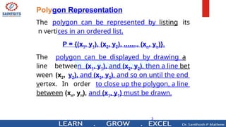
Polygon Representation
The polygon can be represented by listing its
n vertices in an ordered list.
P = {(x1, y1), (x2, y2), ……., (xn, yn)}.
The polygon can be displayed by drawing a
line between (x1, y1), and (x2, y2), then a line bet
ween (x2, y2), and (x3, y3), and so on until the end
vertex. In order to close up the polygon, a line
between (xn, yn), and (x1, y1) must be drawn.

5. Polygon Fill Algorithm
• Different types of Polygons
• Simple Convex
• Simple Concave
• Non-simple : self-intersecting
• With holes
Convex Concave Self-intersecting

6. 5
Polygon Filling
Types of filling
• Solid-fill
All the pixels inside the polygon’s boundary are illu
minated.
• Pattern-fill
The polygon is filled with an arbitrary predefined
pattern.

7. Types of Polygon fill algorithm
• 1.Scan line algorithm
• 2. Boundary Fill algorithm
• 3. Flood fill algorithm

8. 7
The Scan-Line Polygon Fill Algorithm
The scan-line polygon-filling algorithm involves
• the horizontal scanning of the polygon from its
lowermost to its topmost vertex,
• identifying which edges intersect the scan-line,
•and finally drawing the interior horizontal lines
with the specified fill color. process.

9. Example
• Consider the following polygon:

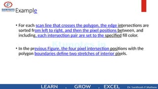
10. Example
• For each scan line that crosses the polygon, the edge intersections are
sorted from left to right, and then the pixel positions between, and
including, each intersection pair are set to the specified fill color.
• In the previous Figure, the four pixel intersection positions with the
polygon boundaries define two stretches of interior pixels.

11. 0
-
+
0
SAI MTGITS can I
i
n
eFill AI aritlom
—Intersect scanline withe d g e s
—Fill b e t w e e n pairsintersections
—B as i c algorithm :
Fory=ymintoy m a x
1) intersect scan line y with each edge
2) sort interesections by increasing x
[pO,p1 ,p2, pS]
3) fill pairwise( p O —» p1 ,p2—» pS,... )

12. SAI NTGITS
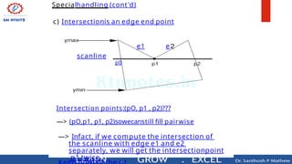
Specialhandling (cont'd)
c) Intersectionis an edge end point
scanline
p0
e1 e
Intersection points:(pO, p1 , p2)???
—> (pO,p1, p1, p2)sowecanstill fill pairwise
—> Infact, if we compute the intersection of
the scanline with edge e1 and e2
separately, we will get the intersectionpoint
p1 twice.

13. Ńw
SAI NTGITS
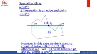
Special handlinq
(cont'd)
c) Intersection is an edge end point
(cont'd)
e1p1
p2
e2
However, in this case we don't want to
count p1 twice (p0,p1,p1,p2,p3),
otherwise we will fill pixels between p1
and p2, which is wrong

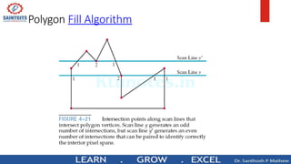
14. Polygon Fill Algorithm
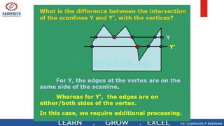
• Consider the next Figure.
• It shows two scan lines that cross a polygon fill area and intersect a
vertex.
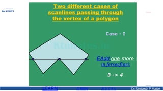
• Scan line y’ intersects an even number of edges, and the two pairs of
intersection points along this scan line correctly identify the interior
pixel spans.
• But scan line y intersects five polygon edges.

15. Polygon Fill Algorithm

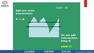
16. Polygon Fill Algorithm
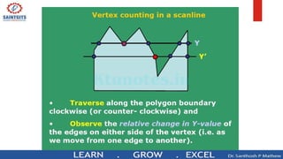
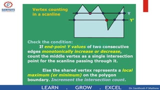
• To identify the interior pixels for scan line y, we must count the vertex
intersection as only one point.
• Thus, as we process scan lines, we need to distinguish between these
two cases.

17. EAdd one more
in fersecfíori:
LEARN G RllIW .E X C E L Dr
. Santízesíz P Matíze
SAI NTGITS

22. Boundary Fill
Algorithm
Introduction :
• Boundary Fill Algorithm starts at a pixel inside the
polygon to be filled and paints the interior pr
oceeding outwards towards the boundary.
• This algorithm works only if the color with which
the region has to be filled and the color of the
boundary of the region are different.
• If the boundary is of one single color, this approach
proceeds outwards pixel by pixel until it hits the
boundary of the region.

23. Boundary Fill
Algorithm
Boundary Fill Algorithm is recursive in nature
• Ittakesaninteriorpoint(x,y),afillcolor, and a
boundary color as the input.
• The algorithm starts by checking the color of (x, y). If
it’s color is not equal to the fill color and the boundary
color, then it is painted with the fill color and the
function is called for all the neighbors of (x, y).
• If a point is found to be of fill color or of boundary
color, the function does not call its neighbors and
returns.
• Thisprocesscontinuesuntilallpointsupto the
boundary color for the region have been tested.
• The boundary fill algorithm can be implemented by 4-
connected pixels or 8-connected pixels.

24. Boundary Fill
Algorithm
4-connected pixels :
• After painting a pixel, the function is called for four neighboring points. These are the
pixel positions that are right, left, above, and below the current pixel. Areas filled by
this method are called 4-connected.
• Algorithm:
void boundaryFill4(int x, int y, int fill_color,int boundary_color)
{
if(getpixel(x, y) != boundary_color &&
getpixel(x, y) != fill_color)
{
putpixel(x, y, fill_color);
boundaryFill4(x + 1, y, fill_color, boundary_color);
boundaryFill4(x, y + 1, fill_color, boundary_color);
boundaryFill4(x - 1, y, fill_color, boundary_color);
boundaryFill4(x, y - 1, fill_color, boundary_color);
}
}

25. Boundary Fill
Algorithm
8-connected pixels :
More complex figures are filled using this approach. The pixels to be tested are the 8 neighboring pixels,
the pixel on the right, left, above, below and the 4 diagonal pixels. Areas filled by this method are called 8-
connected.
Algorithm :
void boundaryFill8(int x, int y, int fill_color,int boundary_color)
{
if(getpixel(x, y) != boundary_color &&
getpixel(x, y) != fill_color)
{
putpixel(x, y, fill_color);
boundaryFill8(x + 1, y, fill_color, boundary_color);
boundaryFill8(x, y + 1, fill_color, boundary_color);
boundaryFill8(x - 1, y, fill_color, boundary_color);
boundaryFill8(x, y - 1, fill_color, boundary_color);
boundaryFill8(x - 1, y - 1, fill_color, boundary_color);
boundaryFill8(x - 1, y + 1, fill_color, boundary_color);
boundaryFill8(x + 1, y - 1, fill_color, boundary_color);
boundaryFill8(x + 1, y + 1, fill_color, boundary_color);
}
}

26. Boundary Fill
Algorithm
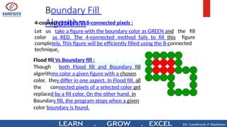
4-connected pixels Vs 8-connected pixels :
Let us take a figure with the boundary color as GREEN and the fill
color as RED. The 4-connected method fails to fill this figure
completely. This figure will be efficiently filled using the 8-connected
technique.
Flood fill Vs Boundary fill :
Though both Flood fill and Boundary fill
algorithms color a given figure with a chosen
color, they differ in one aspect. In Flood fill, all
the connected pixels of a selected color get
replaced by a fill color. On the other hand, in
Boundary fill, the program stops when a given
color boundary is found.

27. Flood Fill Algorithm
• Sometimes we come across an object where we want to fill the
area and its boundary with different colors. We can paint such
objects with a specified interior color instead of searching for
particular boundary color as in boundary filling algorithm.
Instead of relying on the boundary of the object, it relies
on the fill color. In other words, it replaces the interior
color of the object with the fill color. When no more pixels
of the original interior color exist, the algorithm is
completed.
• Once again, this algorithm relies on the Four-connect or Eight-
connect method of filling in the pixels. But instead of looking for
the boundary color, it is looking for all adjacent pixels that are a
part of the interior.

28. Flood Fill Algorithm
• Algorithm (4-connect):
floodfill4 (x, y,fill_ color, old_color: integer)
{
If (getpixel (x, y)=old_color)
{
setpixel (x, y, fill_color);
fill (x+1, y, fill_color, old_color);
fill (x-1, y, fill_color, old_color);
fill (x, y+1, fill_color, old_color);
fill (x, y-1, fill_color, old_color);
}
}

29. Flood Fill Algorithm
• Algorithm:
floodfill8 (x, y,fill_color, old_color: integer)
{
If (getpixel (x, y)=old_color)
{
setpixel (x, y, fill_color);
floodfill(x+1,y,old,newcol);
floodfill(x-1,y,old,newcol);
floodfill(x,y+1,old,newcol);
floodfill(x,y-1,old,newcol);
floodfill(x+1,y+1,old,newcol);
floodfill(x-1,y+1,old,newcol);
floodfill(x+1,y-1,old,newcol);
floodfill(x-1,y-1,old,newcol);
}

30. 2D Transformations

31. 2D Transformations
y


tx

 y


x
    t

P' P  T
 y'

 x'

 4.1
8.2
 

x' 3.4
y' 4.1
 y
'
 x'

 3.7

7.1
x' 3.7  7.1
y' 4.1 8.2
P  (3.7,4.1)
T  (7.1,8.2)
Given:
P  (x, y)
T  (tx , ty )
We want:
x' x  tx
y' y  ty
Matrix form:

32. 2D Transformations

33. 2D Transformations
Rotation:

34. 2D Transformations
Rotation:

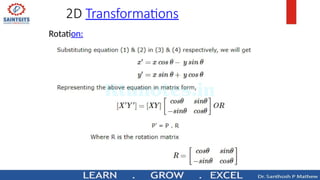
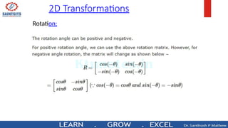
35. 2D Transformations
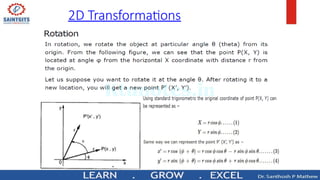
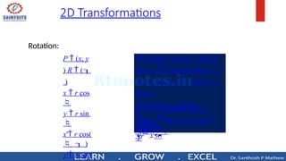
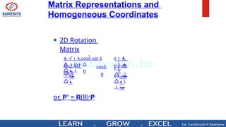
Rotation:
P  (x, y
) R  (
)
x  r cos

y  r sin

x' r cos(
   )
y' r cos(
P' R 
P
 y
'

sin cos


 y

 x'

cos sin 
 x
x' r cos cos  r sin 
sin  y' r cos sin   r
sin  cos x' x cos  y
sin 
y' x sin   y cos

36. 2D Transformations

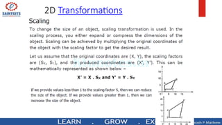
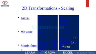
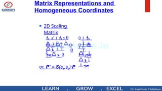
37. 2D Transformations - Scaling
• Given:
• We want:
x
y

y
y 



s




• Matrix form:


P' S 
P
0s
0 x
 y
'
x'
y' sy
x' sx x
P  (x, y)
S  (sx , sy )
0
1.4
3


2.2




x' 4.2
y' 6.6
 y'
0
 x'

3
x' 3*1.4
y' 3*2.2
P 
(1.4,2.2)
S  (3,3)

38.  Many graphics applications involve
sequences of geometric
transformations
Animations
Design and picture construction
applications
 We will now consider matrix
representations of these
operations
Sequences of transformations can
Matrix Representations and
Homogeneous Coordinates

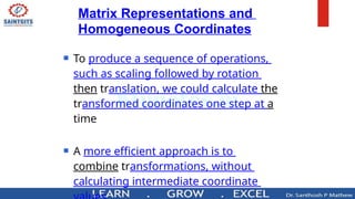
39. Matrix Representations and
Homogeneous Coordinates
 To produce a sequence of operations,
such as scaling followed by rotation
then translation, we could calculate the
transformed coordinates one step at a
time
 A more efficient approach is to
combine transformations, without
calculating intermediate coordinate

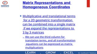
40. Matrix Representations and
Homogeneous Coordinates
 Multiplicative and translational terms
for a 2D geometric transformation
can be combined into a single matrix
if we expand the representations to
3 by 3 matrices
 We can use the third column for
translation terms, and all transformation
equations can be expressed as matrix
multiplications

41. Matrix Representations and
Homogeneous Coordinates
 Expand each 2D coordinate (x,y) to
three element representation (xh,yh
,h) called homogeneous
coordinates
 h is the homogeneous parameter
such thatx = xh/h,y = yh/h,
 A convenient choice is to choose h = 1

42. Matrix Representations and
Homogeneous Coordinates
 2D Translation
Matrix
or, P’ = T(tx,ty)·P

 1 
0
t 
 y
 x'10
 y'  0
1
0
y 

1 
1

tx  x


43. Matrix Representations and
Homogeneous Coordinates
 2D Rotation
Matrix
or, P’ = R(θ)·P


1
1

0

 1


0 
 y
0
x
 y'  
sin 
 x'cos sin 
cos
0

44. Matrix Representations and
Homogeneous Coordinates
 2D Scaling
Matrix
or, P’ = S(sx,sy)·P


1
1

0

 1 
 0
0 
 y
0
x
 y'   0
s
y
 x'sx0

45. 1



0
 
0
1



0
1 




0

0

1y2 y 


1 y

2 y 

10 t2 x 
1t t
0
t1x
t
t1x

t
10t2 x 10
11
00
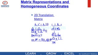
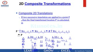
 Composite 2D Translations
 If two successive translation are applied to a point P
, then the final transformed location P' is calculated
as
P '  T(tx2
, ty2
)  T(tx1
, t y1
)  P  T(tx1
 tx2
, t y1
 ty2
)
 P
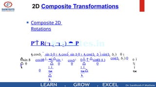
2D Composite Transformations

46. 2D Composite Transformations




1


0



1


0
0
0  sin(  )


1



0
sin  cos0  sin

0
cos(1  2 ) 0
12
0
1
1
2
2
cos2  sin 20cos1 sin 10cos(1  2 ) sin(1  2 ) 0
cos
 Composite 2D
Rotations
P' R(1  2 )  P

47. 2D Composite Transformations
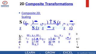
 Composite 2D
Scaling

1


0

0
0
0

0

1

0
0 


1
 0
0



0

0
y1y 2
y1
y 2 s s
0
sx1  s
x 2
0   0
s
00sx100
s
sx
2
2
1
2
1
11
2
2 y
y
xx
y
x
xy ,
s
,
s

s)
)  S (s
 s
)
S (s
S (s,
s

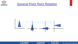
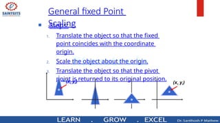
48. General Pivot Point Rotation
 Steps:
1. Translate the object so that the pivot
point is moved to the coordinate origin.
2. Rotate the object about the origin.
3. Translate the object so that the pivot
point is returned to its original position.

49. General Pivot Point Rotation

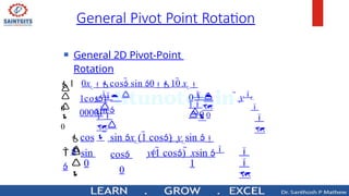
50.  General 2D Pivot-Point
Rotation

1
0
0 
0



0

0
r



r 

1 


 y
y  
sin 
1 0xr cos sin 010 xr 
1cos1
00001






1
0
 sin

cos
 rr
y(1 cos)  xsin 
 sin xr (1 cos)  yr sin 
cos
0
General Pivot Point Rotation

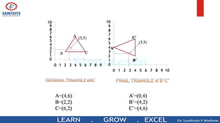
51. Problem:
Given a triangle ABC A(4,6) B(2,2)C(6,2). Rotate it by 90
degree anticlockwise about the point (3,3).
Solution:
We have xr=3 yr=3
R( )=90˚
Ɵ
1.Translate to
origin T(-3,-3).
2. Then Rotate
anticlockwise.
3.Translate back
to original
position T(3,3)

52. LEARN G ROW .E X C E L Dr
. Santízesíz P Matíze
SAI NTGITS
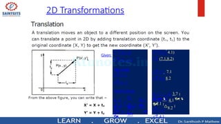
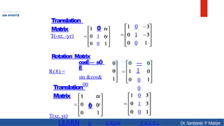
Translation
Matrix 0
T(-xr, -yr) 1
0
R(8) =
Rotation Matrix
cosË— sÔ
Ë
sin &cos&
00
Translation
Matrix
0
T(xr, yr)
0
0
1
0
—
1
0
0
0
1
0

53. rr 





1
0
y(1 cos)  xsin o
 sin xr (1 cos)  yr sin 
cos
0
cos

o' sin


55. So as we have substituted all the values in the corresponding matrices. We
will arrange them in sequence. Always keep in mind matrix multiplication
is associative but not commutative. Arrange them from right to left and
object matrix being the rightmost.

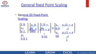
56.  Steps:
1. Translate the object so that the fixed
point coincides with the coordinate
origin.
2. Scale the object about the origin.
3. Translate the object so that the pivot
point is returned to its original position.
General fixed Point
Scaling
(xr, yr) (xr, yr)

57. 1 0
𝑥𝑓
0 1
𝑦𝑓
0 0 1
𝑠𝑥 0
0
.0 𝑠𝑦 0
001
1 0 −
𝑥𝑓
.0 1 − 𝑦
𝑓
0 01
=
𝑠𝑥
0 0
𝑠𝑦
00
𝑥𝑓(1 − 𝑠
𝑥)
𝑦𝑓(1 − 𝑠
𝑦)
1
• General 2D Fixed-Point
Scaling:
General fixed Point Scaling

58.  Reflection
 Transformation that produces a mirror image
of an object
Other 2D Transformations

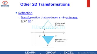
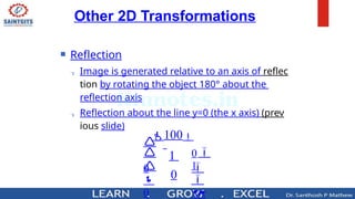
59.  Reflection
 Image is generated relative to an axis of reflec
tion by rotating the object 180° about the
reflection axis
 Reflection about the line y=0 (the x axis) (prev
ious slide)

1





0
0


0
100
1
0
Other 2D Transformations

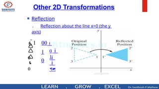
60.  Reflection
 Reflection about the line x=0 (the y
axis)

1





0
0


0
1 00
1
0
Other 2D Transformations

61.  Reflection about the
origin
−1 00
0 − 10
0 01
Other 2D Transformations

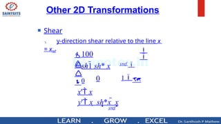
62. Other 2D Transformations
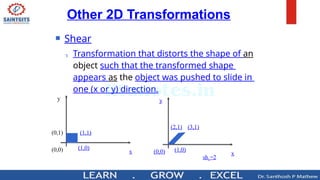
 Shear
 Transformation that distorts the shape of an
object such that the transformed shape
appears as the object was pushed to slide in
one (x or y) direction.
y
x
(0,1) (1,1)
(1,0)
(0,0)
y
x
(2,1) (3,1)
(1,0)
(0,0)
shx=2

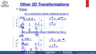
63.  Shear
 An x-direction shear relative to the x
axis
 An y-direction shear relative to the y
axis

1



0
0

100
y
sh1
0

1





0
0

1shx0
1
0
x
y' y
x' x  sh y
Other 2D Transformations
y' y  shy 
x x' x
x’
y’
1
=
0
x
y
1
x’
y’
1
=
x
y
1

64. LEARN G ROW .E X C E L Dr
. Santízesíz P Matíze
BAIRTBITS
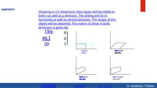
Shearing in X-Y directions: Here layers will be slided in
both x as well as y direction. The sliding will be in
horizontal as well as vertical direction. The shape of the
object will be distorted. The matrix of shear in both
directions is given by:
1Shy
ss,i
00
Original
Object
Shear in Y
direction
Shear in X
direction
Shear in both
direcaons

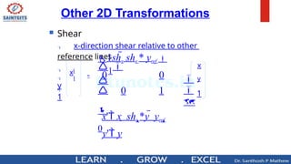
65.  Shear
 x-direction shear relative to other
reference lines

xl

y
l

1
x
y
1






0
0
1
0
1shx shx * yref 
1
0
x' x  shx *y  yref 
y' y
Other 2D Transformations
=

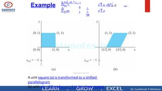
66. A unit square (a) is transformed to a shifted
parallelogram
(b) with shx = 0.5 and yref = 1
− in the shear matrix
Example 


0
1
1shx shx * yref 
01

00
ref
x
y' y
x' x  sh*y  y 

67.  Shear
 y-direction shear relative to the line x
= xref


0
100


yref 
1
y
sh1 sh* x
0
x' x
y' x  sh*x  x
yref
Other 2D Transformations

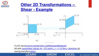
68. Other 2D Transformations –
Shear - Example
A unit square (a) is turned into a shifted parallelogram
(b) with parameter values shy = 0.5 and xref = 1
− in the y -direction sh
earing transformation

69. Basic 3D Transformations
o
Scaling:
o
Rotation:

0
o Translation:
1 t
0


0
0tx 
1y 
01 

00
y
s



0

sx
0


 001
cos sin 0
sin cos

001
Recap – 2D Transformations

70. 
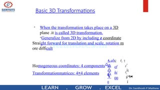
When the transformation takes place on a 3D
plane .it is called 3D transformation.

Generalize from 2D by including z coordinate
Straight forward for translation and scale, rotation m
ore difficult
Transformationmatrices: 4×4 elements

 1


0
y

tz



g
t

Homogeneous coordinates: 4 componentsd
abc tx 
ef
hi
00
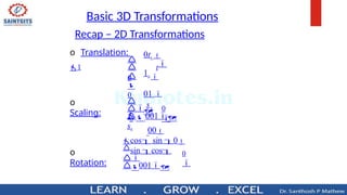
Basic 3D Transformations

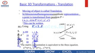
71. Basic 3D Transformations - Translation

Moving of object is called Translation.

In3dimensionalhomogeneouscoordinate representation ,
a point is transformed from position P =
( x, y , z) to P’=( x’, y’, z’)

This can be written
as:- Using P’ = T . P



 
 


1

1

100
10
01
00
t y


z
0
 1

0
 y
0

x
 tz

z 
y  

tx 
x

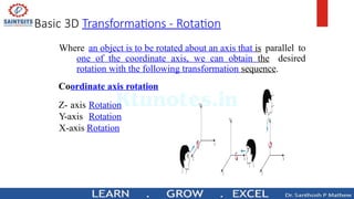
72. Basic 3D Transformations - Rotation
Where an object is to be rotated about an axis that is parallel to
one of the coordinate axis, we can obtain the desired
rotation with the following transformation sequence.
Coordinate axis rotation
Z- axis Rotation
Y-axis Rotation
X-axis Rotation

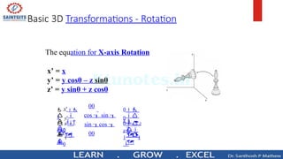
73. Basic 3D Transformations - Rotation
The equation for X-axis Rotation
x’ = x
y’ = y cosθ – z sinθ
z’ = y sinθ + z cosθ
 



  

 

00
cos  sin 
sin cos 
00
0 z

11

0
y
0
x
 z'
0
 1 
0
 y'
0
 x'
1

74. Basic 3D Transformations - Rotation
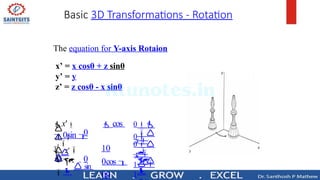
The equation for Y-axis Rotaion
x’ = x cosθ + z sinθ
y’ = y
z’ = z cosθ - x sinθ






 


0
0
 1

0
z 
1
1
0
y
0
x
 z'
 sin

y'

x'  cos
0sin 
10
0cos 
00

75. Basic 3D Transformations - Rotation
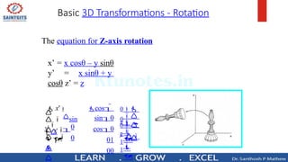
The equation for Z-axis rotation
x’ = x cosθ – y sinθ
y’ = x sinθ + y
cosθ z’ = z
 




 
 


0
0
 1


0
z 
1

1

0
y
0
x
 z'


y'
sin

 x' cos
sin0
cos0
01
00

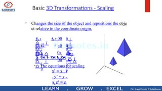
76. Basic 3D Transformations - Scaling

Changes the size of the object and repositions the obje
ct relative to the coordinate origin.




 

0
 z

1

1

0
 y

0
x

 z

0
 1

 0
 y
 0
x

y
sx00
s0
0sz
00

The equations for scaling
x’ = x . s
x y’ = y .
sy z’ = z
. sz

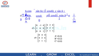
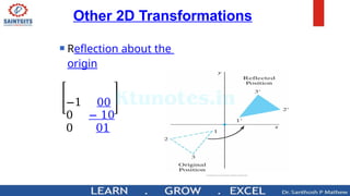
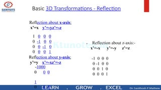
77. Basic 3D Transformations - Reflection
Reflection about x-axis:
x’=x y’=-yz’=-z
R
1 0 0 0
0 -1 0 0
0 0 -1 0
0 0 0 1
eflection about y-axis:
y’=y x’=-xz’=-z
-1000
0
1
0 0
0 -1 0