Compressible Flow.pptCompressible Flow.ppt

1. Compressible Flow
 Density might not be constant when the flow velocity is
high. How high? In general, the compressibility effect is
proportional to the square of Mach number ~ M2
.
Therefore, for the case of M=0.3, it will contribute to
roughly 10% error by neglecting compressibility effect.
 Usually, temperature variation can be significant when the
flow velocity is high. Consequently, energy equation is
important also.
 The relationship between temperature and density can still
be characterized by the ideal gas model. (might not be
valid for extremely high speed flow)
 In this class, most flow analysis discussed will be
considered as one-dimensional for simplicity. However, it
is understood that multi-dimensional effect can be
significant in real flow configurations.

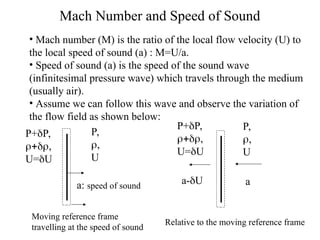
2. Mach Number and Speed of Sound
• Mach number (M) is the ratio of the local flow velocity (U) to
the local speed of sound (a) : M=U/a.
• Speed of sound (a) is the speed of the sound wave
(infinitesimal pressure wave) which travels through the medium
(usually air).
• Assume we can follow this wave and observe the variation of
the flow field as shown below:
a: speed of sound
P+P,
,
U=U
P,
,
U
Moving reference frame
travelling at the speed of sound
a
a-U
P+P,
,
U=U
P,
,
U
Relative to the moving reference frame

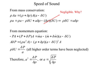
3. Speed of Sound
2 2
From mass conservation:
( ) ( )
( )( )
From momentum equation:
( ) ( )( )
( ) ( )( )
(all higher order terms have been neglected)
Aa A a U
a a U a U U a
PA P P A ma m m a U
A P a A a U A
P
U
a
   
       
  
    


  
     
      
   

  
2
Therefore, , or
P P
a a
 
 
 
Negligible. Why?

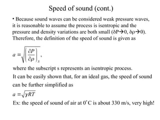
4. Speed of sound (cont.)
• Because sound waves can be considered weak pressure waves,
it is reasonable to assume the process is isentropic and the
pressure and density variations are both small (P0, 0).
Therefore, the definition of the speed of sound is given as
,
where the subscript s represents an isentropic process.
It can be easily shown that, for an ideal gas, the speed of sound
can be further simplified as
Ex: the speed of sound of air a
S
P
a
a RT


 

  

 

t 0 C is about 330 m/s, very high!


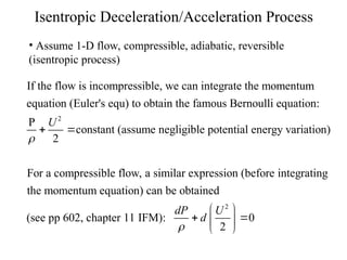
5. Isentropic Deceleration/Acceleration Process
• Assume 1-D flow, compressible, adiabatic, reversible
(isentropic process)
2
If the flow is incompressible, we can integrate the momentum
equation (Euler's equ) to obtain the famous Bernoulli equation:
P
constant (assume negligible potential energy variation)
2
For a compress
U

 
2
ible flow, a similar expression (before integrating
the momentum equation) can be obtained
(see pp 602, chapter 11 IFM): 0
2
dP U
d

 
 
 
 

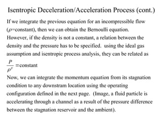
6. Isentropic Deceleration/Acceleration Process (cont.)
If we integrate the previous equation for an incompressible flow
( =constant), then we can obtain the Bernoulli equation.
However, if the density is not a constant, a relation between the
density and

the pressure has to be specified. using the ideal gas
assumption and isentropic process analysis, they can be related as
constant
Now, we can integrate the momentum equation from its stagnation
co
P



ndition to any downstram location using the operating
configuration defined in the next page. (Image, a fluid particle is
accelerating through a channel as a result of the pressure difference
between the stagnation reservoir and the ambient).

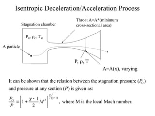
7. Isentropic Deceleration/Acceleration Process
Stagnation chamber
PO, O, TO
P, , T
Throat A=A*(minimum
cross-sectional area)
A=A(x), varying
A particle
O
( 1)
2
It can be shown that the relation between the stagnation pressure ( )
and pressure at any section ( ) is given as:
1
1 , where M is the local Mach number.
2
O
P
P
P
M
P


 

 
 
 
 

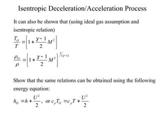
8. Isentropic Deceleration/Acceleration Process
2
1
( 1)
2
It can also be shown that (using ideal gas assumption and
isentropic relation)
1
1
2
1
1
2
Show that the same relations can be obtained using the following
energy equation:
O
O
T
M
T
M
h


 



 
 
 
 

 
 
 
 
2 2
, or
2 2
O p O p
U U
h c T c T
   