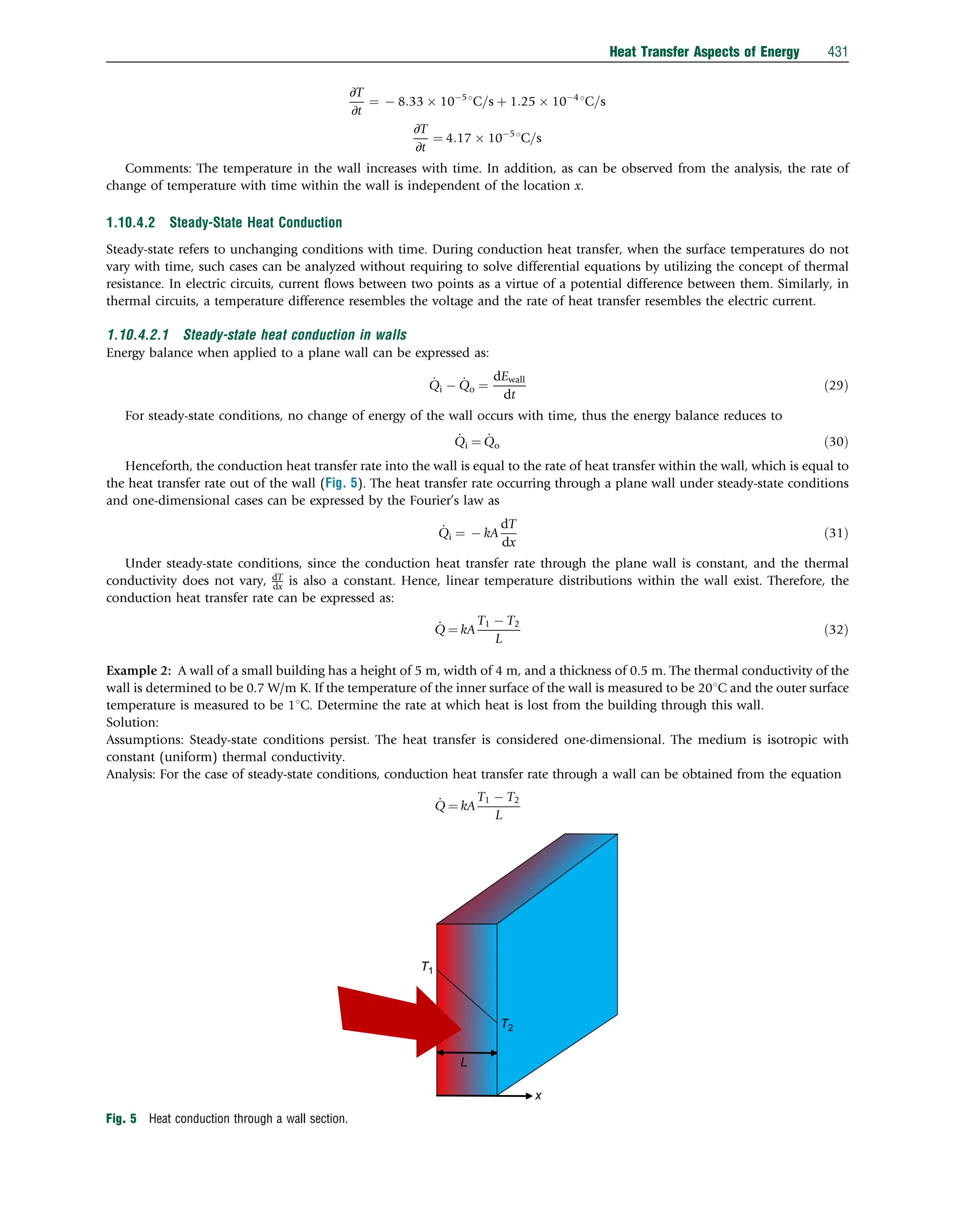
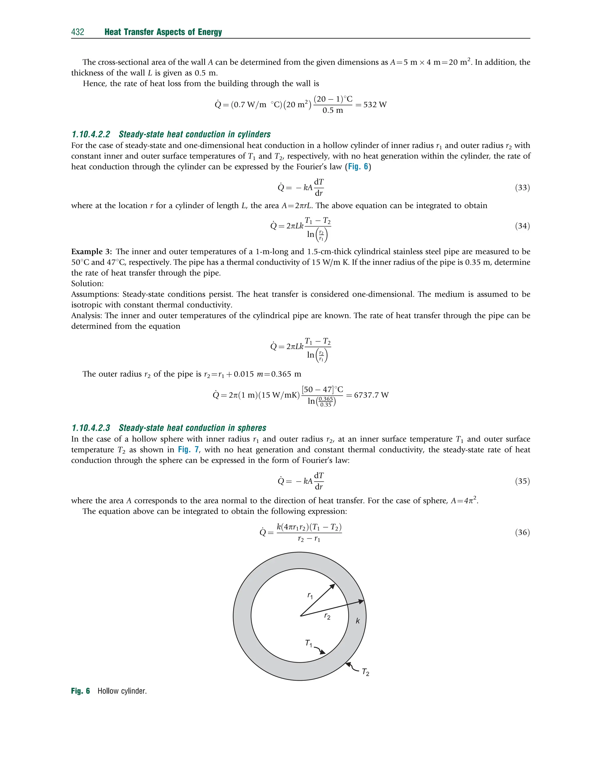
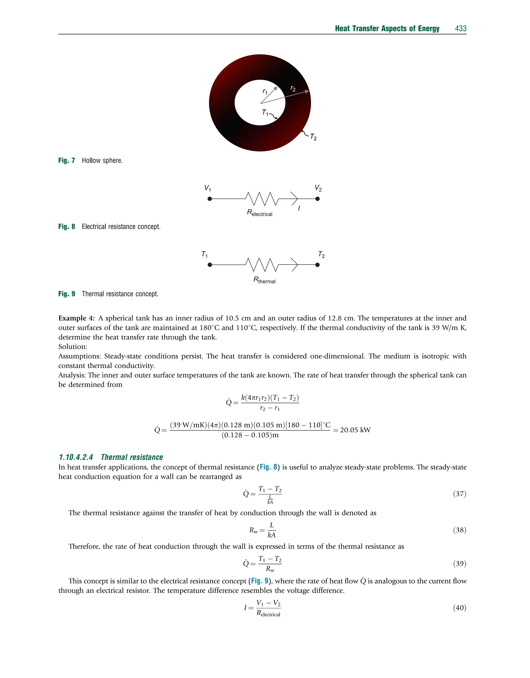
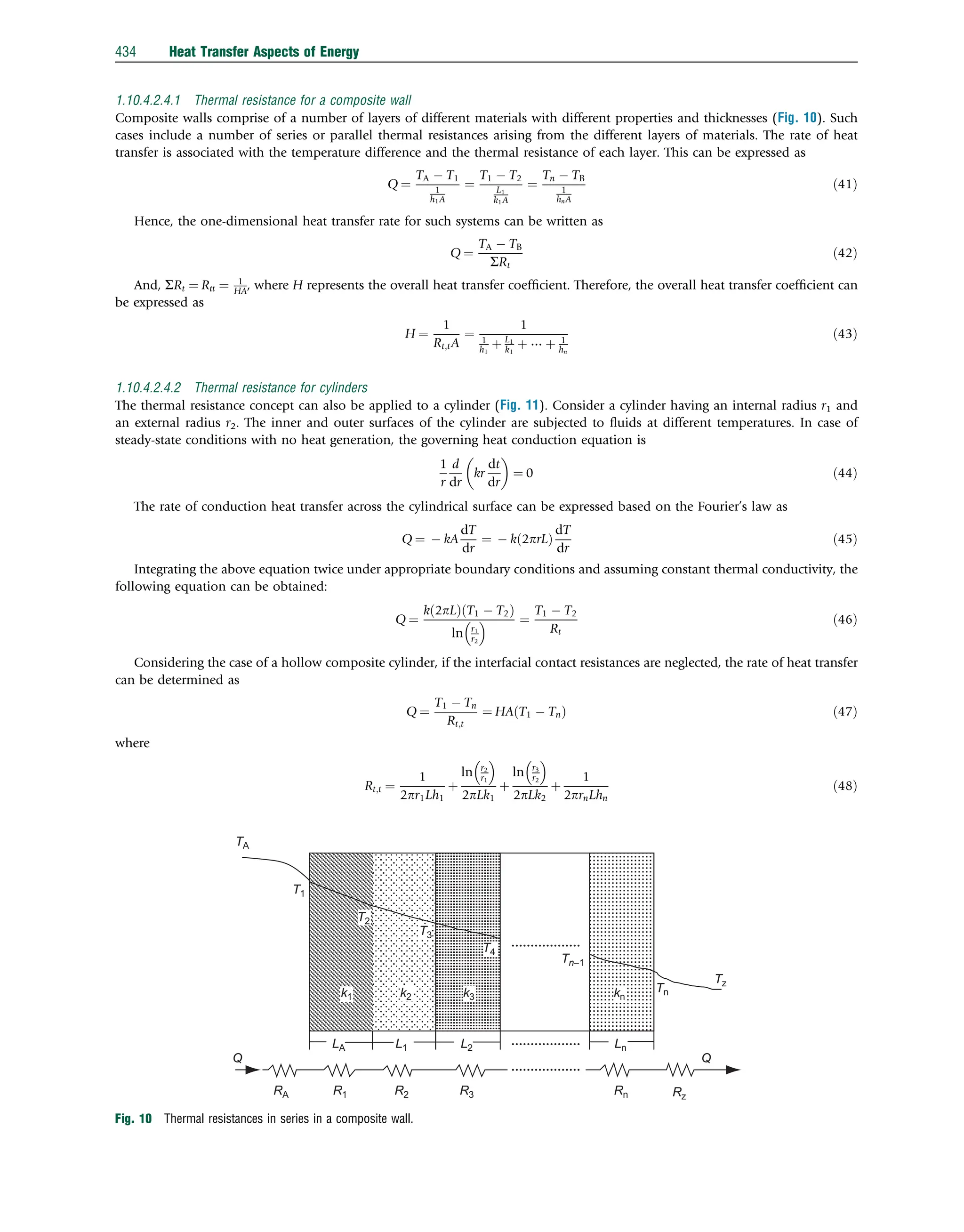
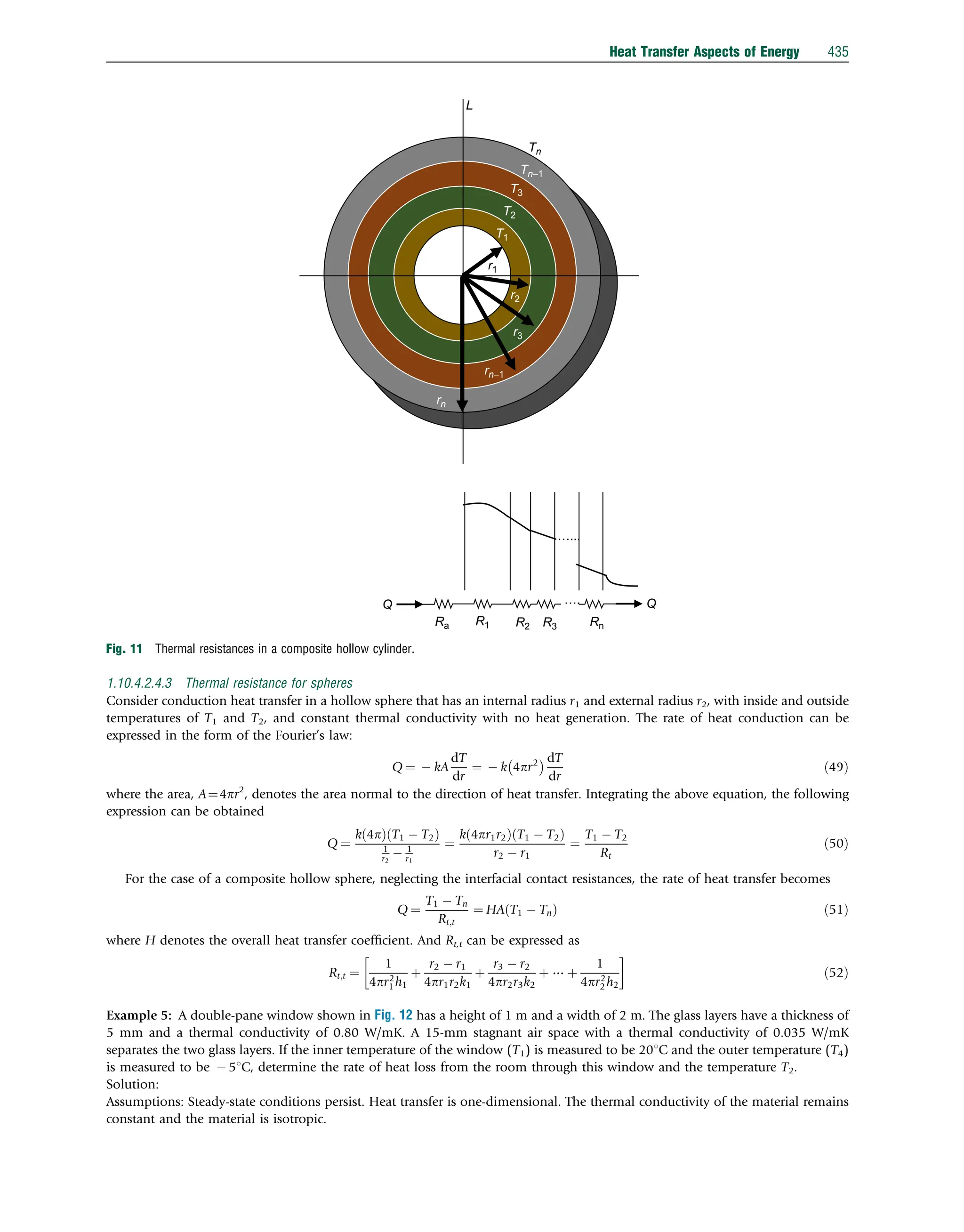
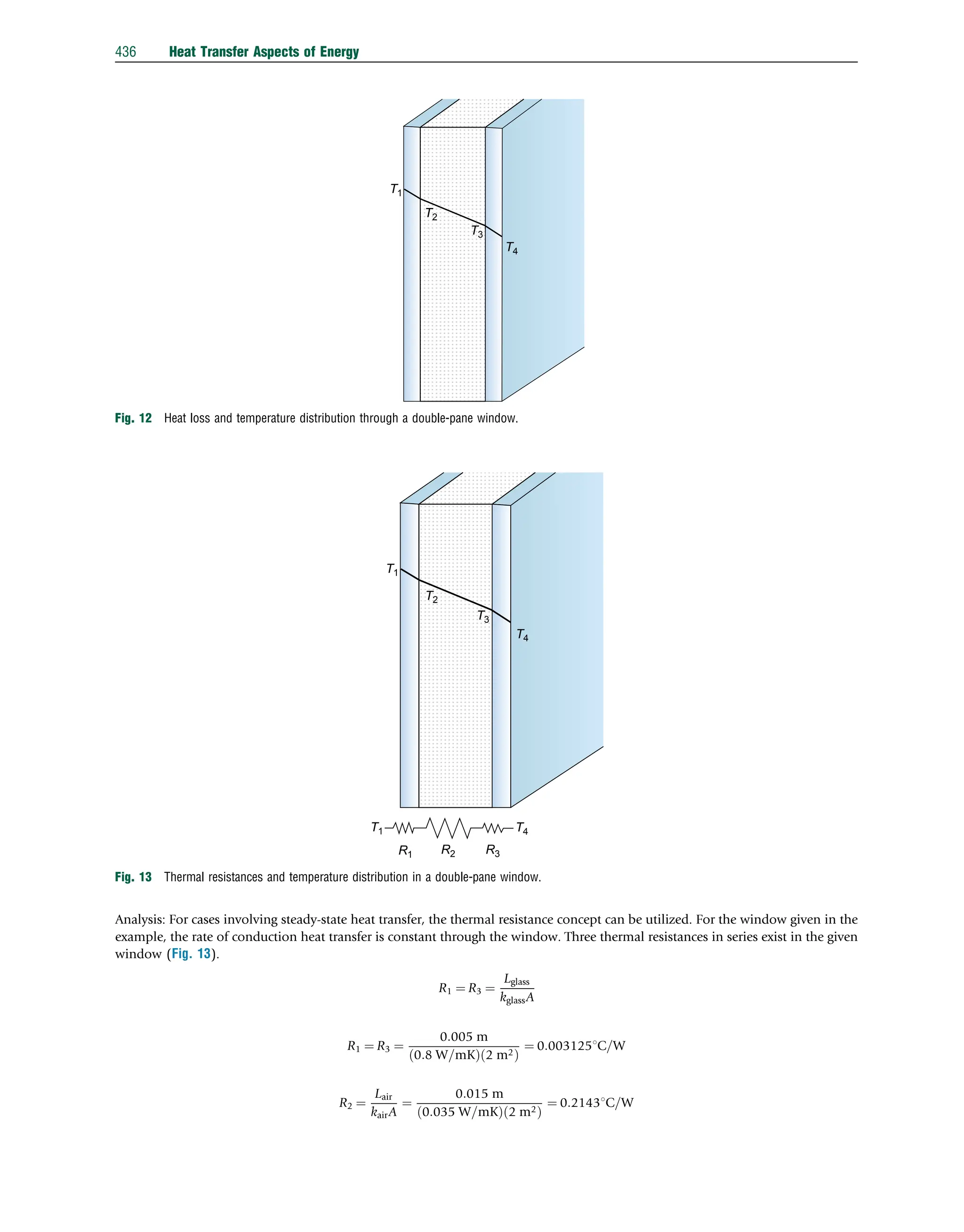
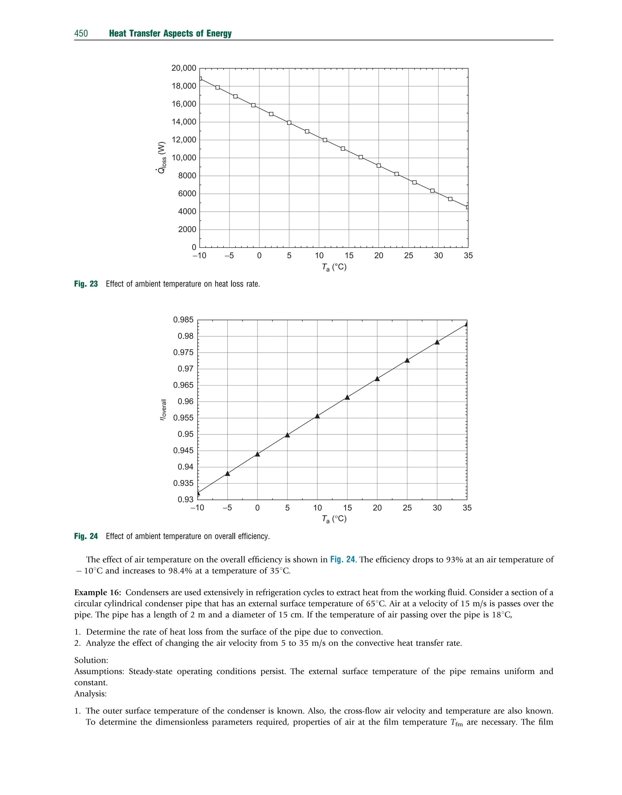
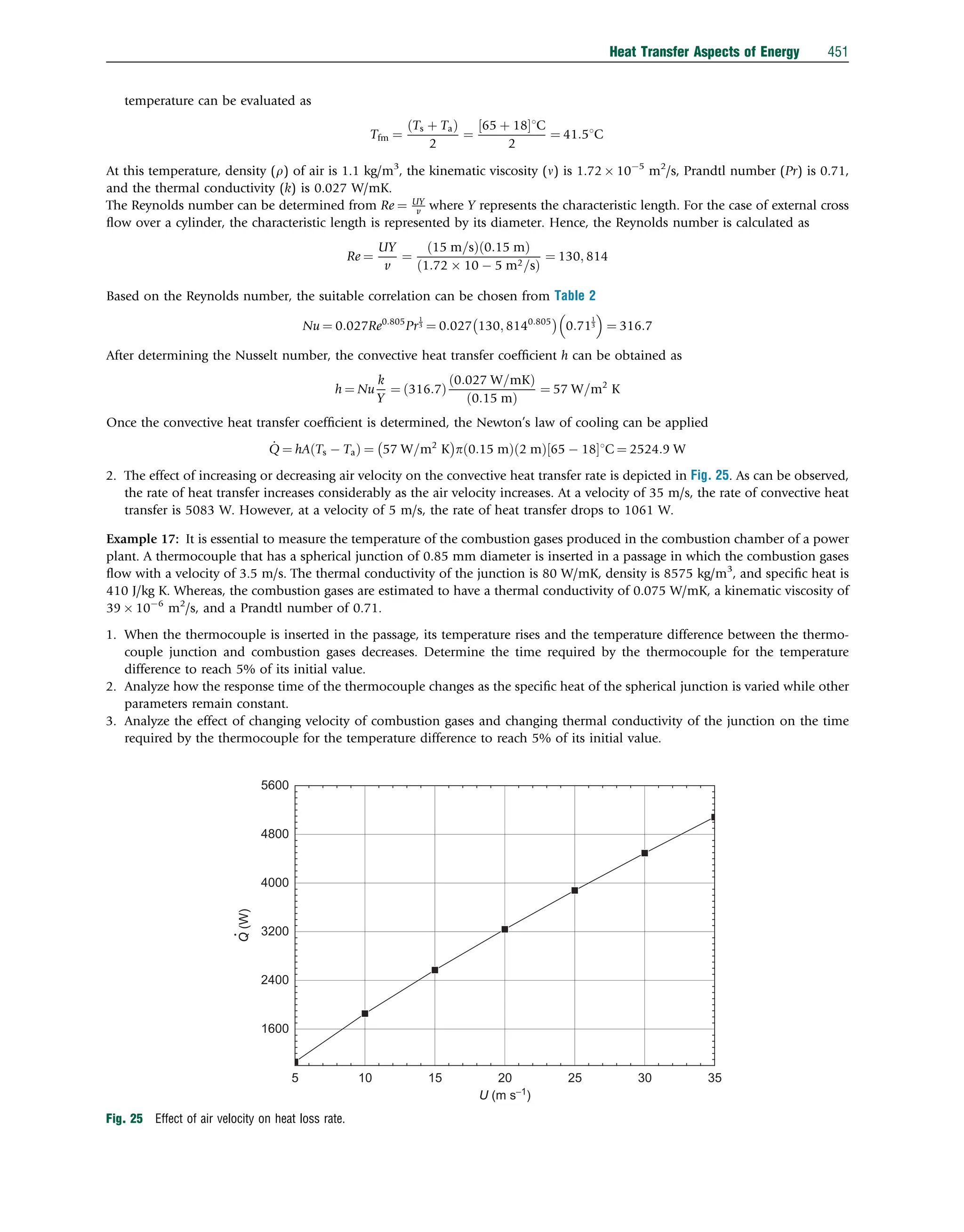
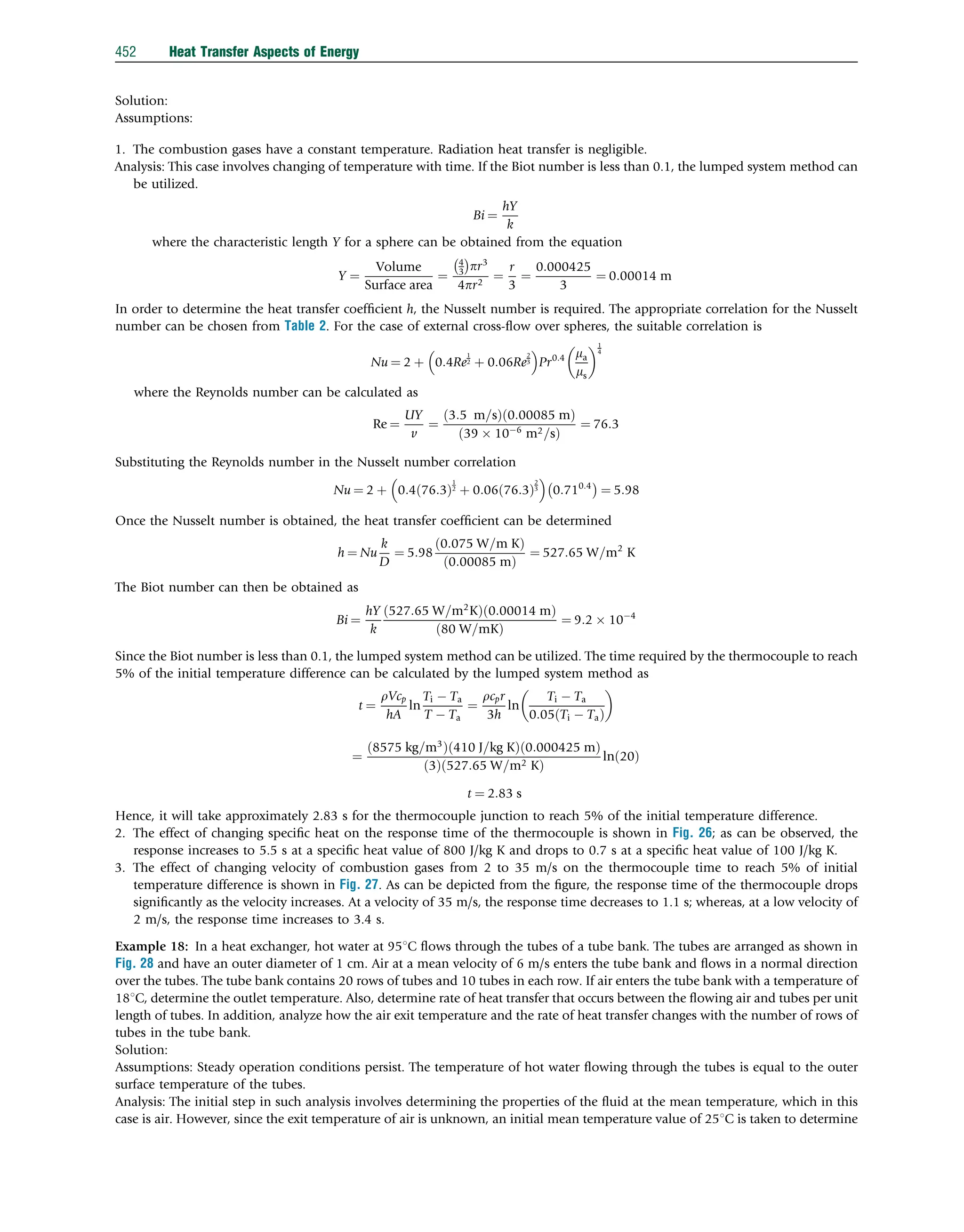
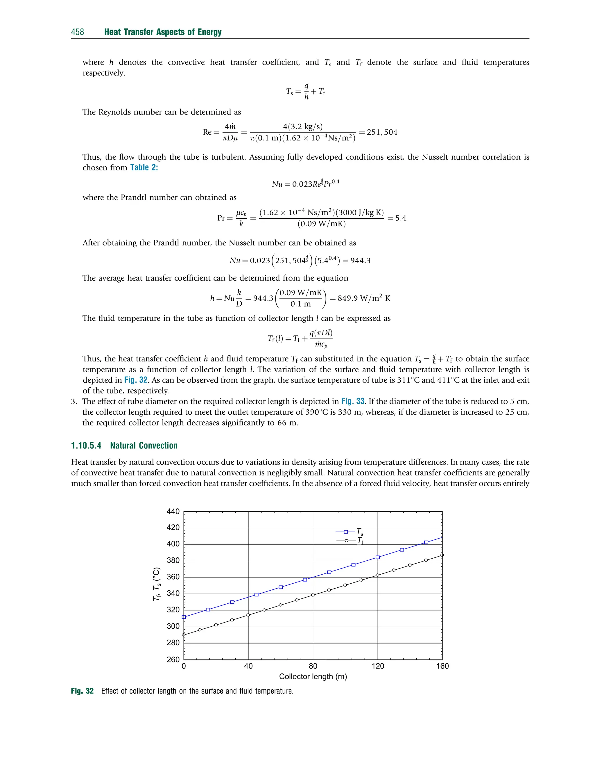
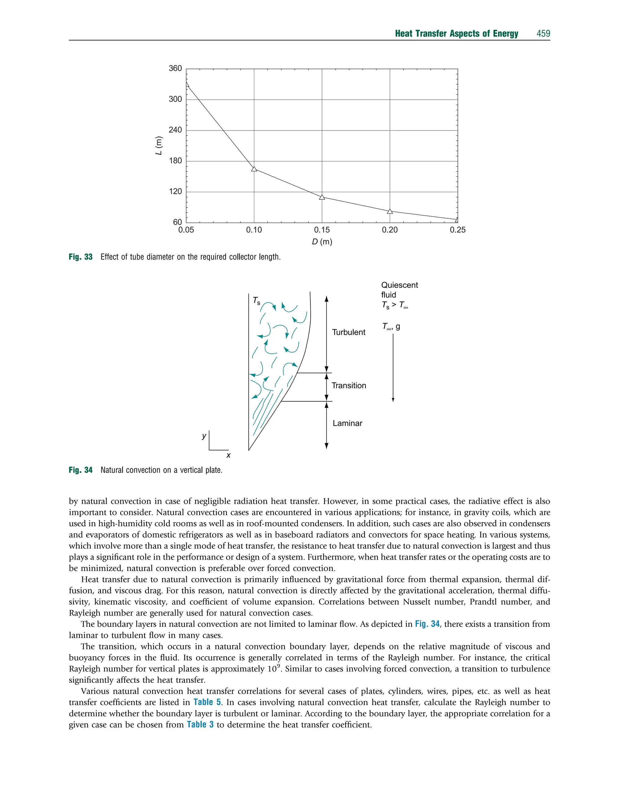
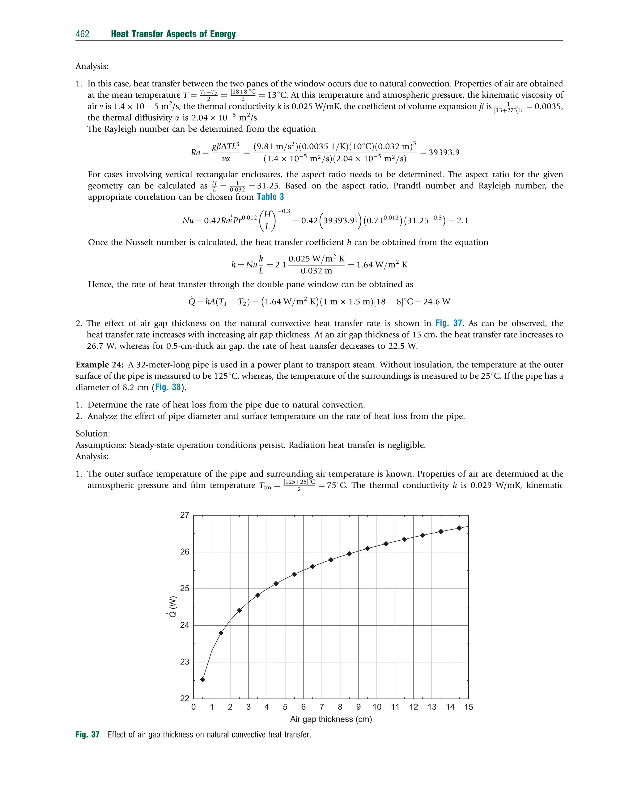
This document discusses heat transfer aspects of energy. It begins by introducing heat transfer and the underlying thermodynamic principles. The first law of thermodynamics states that energy cannot be created or destroyed, only changed from one form to another. Heat transfer occurs between bodies or systems at different temperatures until thermal equilibrium is reached. Various heat transfer mechanisms such as conduction, convection, and radiation are then examined. Case studies on heat exchangers and solar collectors are also presented to demonstrate applications of heat transfer concepts.

1. 1.10 Heat Transfer Aspects of Energy
Ibrahim Dincer and Osamah Siddiqui, University of Ontario Institute of Technology, Oshawa, ON, Canada
r 2018 Elsevier Inc. All rights reserved.
1.10.1 Introduction 424
1.10.2 Thermodynamics and Laws 424
1.10.2.1 First Law of Thermodynamics 425
1.10.2.1.1 Energy balance 425
1.10.2.1.2 Energy balance of closed systems 425
1.10.2.1.3 Energy and mass balance of control volumes 425
1.10.2.2 Second Law of Thermodynamics 426
1.10.3 Heat Transfer 427
1.10.3.1 Classification of Heat Transfer 427
1.10.4 Conduction Heat Transfer 429
1.10.4.1 Heat Conduction Equation 430
1.10.4.2 Steady-State Heat Conduction 431
1.10.4.2.1 Steady-state heat conduction in walls 431
1.10.4.2.2 Steady-state heat conduction in cylinders 432
1.10.4.2.3 Steady-state heat conduction in spheres 432
1.10.4.2.4 Thermal resistance 433
1.10.4.2.4.1 Thermal resistance for a composite wall 434
1.10.4.2.4.2 Thermal resistance for cylinders 434
1.10.4.2.4.3 Thermal resistance for spheres 435
1.10.4.3 Transient Heat Conduction 437
1.10.5 Convection Heat Transfer 442
1.10.5.1 Newton’s Law of Cooling 443
1.10.5.2 The Nusselt Number 445
1.10.5.3 Forced Convection 445
1.10.5.3.1 External flow forced convection 446
1.10.5.3.2 Internal flow forced convection 454
1.10.5.4 Natural Convection 459
1.10.5.5 Boiling Heat Transfer 464
1.10.5.5.1 Pool boiling 464
1.10.5.5.2 Flow boiling 465
1.10.5.6 Condensation Heat Transfer 466
1.10.5.7 Heat Exchangers 466
1.10.6 Radiation Heat Transfer 470
1.10.6.1 The Stefan–Boltzmann Law 471
1.10.7 Case Study 1: Determining the Overall Heat Loss Coefficient for a Flat Plate Solar Collector 473
1.10.8 Case Study 2: Heat Transfer in Parallel-Flow and Counter-Flow Heat Exchangers 475
1.10.9 Future Directions 476
1.10.10 Conclusions 477
References 477
Further Reading 477
Relevant Websites 477
Nomenclature
a Acceleration, m/s2
; absorptivity
A Cross-sectional area, m2
; surface area, m2
Bi Biot number
C Experimental constant
cp Constant-pressure specific heat, kJ/kg K
cv Constant-volume specific heat, kJ/kg K
c0
Specific heat ratio
D Diameter, m
e Specific energy, J/kg or kJ/kg
E Energy, J or kJ
Ex Exergy, J or kJ
F Force; drag force, N
Fo Fourier number
g Acceleration due to gravity (¼9.81 m/s2
)
Gr Grashof number
h Specific enthalpy, kJ/kg; heat transfer coefficient,
W/m2
1C; head, m
H Enthalpy, kJ; overall heat transfer coefficient,
W/m2
1C; head, m
Comprehensive Energy Systems, Volume 1 doi:10.1016/B978-0-12-809597-3.00109-7
422

2. I Electric current, A
k Thermal conductivity, W/m 1C
L Thickness, m; length, m
m Mass, kg; parameter for extended surface;
constant
_
m Mass flow rate, kg/s
n Mole number, kmol
Nu Nusselt number
P Perimeter, m;
Pe Peclet number
PE Potential energy, W or kW
Pr Prandtl number
q Heat rate per unit area, W/m2
; flow rate per unit
width or depth
qh Heat generation per unit volume, W/m3
Q Heat transfer, J or kJ
_
Q Heat transfer rate, W or kW
r Reflectivity; radial coordinate; radial distance, m
Rt Thermal resistance, 1C/W
Ra Rayleigh number
Re Reynolds number
s Specific entropy, kJ/kg
S Entropy, kJ/K
St Stanton number
t Time, s; transmissivity
T Temperature, 1C or K
Ts Absolute temperature of the object surface, K
u Specific internal energy, kJ/kg; velocity in x
direction, m/s; variable velocity, m/s
U Internal energy, kJ; flow velocity, m/s
v Specific volume, m3
/kg; velocity in y
direction, m/s
V Volume, m3
; velocity, m/s
Vr Velocity in radial direction, m/s
Vx Velocity in x direction, m/s
Vy Velocity in y direction, m/s
Vz Velocity in z direction, m/s
Vy Tangential velocity, m/s
_
V Volumetric flow rate, m3
/s
W Work, J or kJ
_
W Rate of work, W or kW
x Quality, kg/kg; Cartesian coordinate; variable
Y Characteristic length, m
z Height, m
Greek letters
b Volumetric coefficient of thermal expansion, 1/
K
δ Increment; difference
D Change in quantity
e Surface emissivity, Eddy viscosity
Z Efficiency
y Dimensionless transient temperature; angle
f Dimensionless heat transfer rate
m Dynamic viscosity, kg/ms; root of the
characteristic equation
n Kinematic viscosity, m2
/s
p Pi number (¼3.1416)
r Density, kg/m3
s Stefan–Boltzmann constant, W/m² K4
; electrical
conductivity, 1/ohm m, surface tension
S Summation
t Shear stress, N/m2
Subscripts and superscripts
a Air; medium; surroundings
av Average
A Fluid A
b Black
B Fluid B
c Cross-sectional, convection, critical
cd Conduction
cn Condensation
cs Control surface
cv Control volume
des Destroyed
dw Dropwise
D Diameter
e Electrical; end; exit
f Fluid; final; flow; force; friction
fg Vaporization
fm Film condition
gen Generation
hg Heater geometry
hs Heat storage
H High-temperature
ie Internal energy
i In
in Input
inc Inclined
j Node
l Liquid
lat Latent
liq Liquid
L Low-temperature
m Midplane for plane wall; centerline for cylinder
mix Mixture
n nth value
nb Nonblack
N nth number
o Out
out Output
p Previous
r Radiation
s Surface; near surface; saturation; free stream; in
direction parallel to streamline
sen Sensible
sf Surface-fluid
sys System
t Total
Heat Transfer Aspects of Energy 423

3. th Thermal
tot Total
tur Turbulent
v Vapor
vap Vapor
ver Vertical
wl Wavy laminar
x x direction
y y direction
z z direction
0 Surroundings; ambient; environment; reference
1 First value; 1st state; initial
1, 2, 3 Points
1.10.1 Introduction
The energy of a system constitutes various forms including thermal, chemical, electrical, magnetic, nuclear, kinetic, or potential
energy. Macroscopic forms of energy are possessed by a system as a whole compared to a specified outside reference. Potential and
kinetic energies are examples of macroscopic energy forms. Whereas, the forms of energy associated with the molecular structure
and level of activity are termed as microscopic forms of energy. The internal energy of a system is defined as the sum of all
microscopic energy forms. These include sensible, latent, chemical, and nuclear energy. Sensible energy is related to the kinetic
energies of molecules, whereas latent energy is associated with the phase of the system. Chemical energy relates to the atomic
bonds of a molecule and nuclear energy, which is associated with the bonds within the atomic nucleus.
When a system gains heat, its thermal energy content rises. This is attributed to the increase in molecular activity of the system.
The temperature of a given system reflects the thermal energy content contained by the system. When two bodies are at different
temperatures, a transfer of energy occurs between them until a thermal equilibrium is established.
Heat transfer is defined as energy flow between systems or bodies due to the presence of a temperature difference between
them. The study of heat transfer involves determining the rate at which energy flows in the form of heat between these bodies
having a temperature gradient. The heat transfer rate between any two given bodies is dependent on the existing temperature
gradient. Ranging from core industrial processes to everyday household devices, the study of heat transfer is applied in a wide
variety of applications and industries.
Analysis of heat transfer between systems is based upon the conservation of energy principle, which states energy cannot be created
or destroyed; rather it only changes from one form to another. The first law of thermodynamics is also an assertion of the principle of
conservation of energy. It avers energy as a thermodynamic property. Thermodynamic properties are quantities that either represent
the attributes of a complete system or are functions of position that is continuous and does not change rapidly over microscopic
distances, except in case of abrupt changes at system boundaries between phases of the given system. Examples of thermodynamic
properties include temperature, pressure, volume, viscosity, etc. Thermodynamic aspects deal with quantifying the amount of heat
transferred from one body to another, whereas heat transfer studies focus on determining the rate at which the heat is transferred.
The objective of this chapter is to present the heat transfer aspects of energy. The underlying thermodynamic principles are
discussed first, and then followed by heat transfer mechanisms, concepts, and application examples.
1.10.2 Thermodynamics and Laws
The term thermodynamics originates from the Greek word “therme” meaning heat and dunamis meaning power. Essentially, it can
be defined as the science of energy that includes all characteristics of energy transformations. When two bodies at different
temperatures are brought in contact with each other, transfer of energy occurs between them until a thermal equilibrium is
established. The Zeroth Law of Thermodynamics asserts that if system A and system B are in thermal equilibrium with a third
system C, this signifies systems A and B are in thermal equilibrium with each other. The First Law of Thermodynamics is essentially
an avowal of the law of conservation of energy, which simply asserts energy transforms from one form to another, but cannot
be created or destroyed. The first law is associated with the amount of heat transfer between two systems or bodies; however, the
direction in which energy transfer occurs is not specified. The Second Law of Thermodynamics avers that energy not only has a
quantity, but also has an associated quality. The direction in which processes occur is determined by the direction in which the
quality of energy decreases. In addition, the second law also determines theoretical performance and efficiency limits of energy
systems. The Third Law of Thermodynamics asserts that any system would attain its minimum possible energy content at absolute
zero temperature. The study of thermodynamics with a macroscopic approach, which does not entail an in depth study of the
behavior of microscopic particles, is termed as classical thermodynamics; whereas, the approach of study that takes the micro-
scopic molecular activity into consideration is known as statistical thermodynamics.
1.10.2.1 First Law of Thermodynamics
As stated above, the first law of thermodynamics asserts that energy cannot be created or destroyed; and it can only change from
one form to another. This principle allows the analysis of the process of energy transfer between a system and its surroundings by
applying an energy balance.
424 Heat Transfer Aspects of Energy

4. It is essential to identify the different forms of energy that may be transferred to or from a system. For any given system, energy
is transferred to the system or is extracted from the system in the form of heat, work, or mass flow. In addition, energy gain or loss
occurs at the system boundary. When heat transfer occurs to a system, there is a rise in the molecular energy. This leads to an
increase in the internal energy of the system. Whereas, when heat transfer occurs from the system to a given surrounding, the
internal energy of the system decreases as the energy contained within the molecules is decreased. Energy transfer by work can be
understood as the transfer of energy to or from a system that does not occur due to a temperature difference between a given
system and its surroundings. When work is done by the system, it results in a decrease in the energy of the system and when work
is performed on the system, it increases the system’s energy. Mass flow is also a mechanism for transfer of energy. When mass flows
into a given system, the energy content of the system is increased due to the amount of energy carried by the mass entering the
system. Similarly, when a mass outflow occurs, it causes a decrease in the energy of the system.
1.10.2.1.1 Energy balance
During any process, the difference between the total amount of energy entering and leaving a system is the equal to the net total
energy change of the system. This is known as the energy balance, which can be expressed as:
Ei Eo ¼ DEsys ð1Þ
where Ei and Eo represent the amount of energy entering and leaving the system, respectively, and DEsys represents the change in
the total energy of the system.
When applied on a unit time basis, it can be written as:
_
Ei _
Eo ¼
dEsys
dt
ð2Þ
Energy balance can be applied to any type of system for any type of process. In order to apply, it requires an identification and
quantification of all types and forms of energy entering or leaving the system.
In the analysis of heat transfer processes, only the energy transfer in the form of heat due to the presence of a temperature
gradient between bodies is considered. Hence, for such analyses a heat balance is expedient:
Qi Qo þ Qgen ¼ DEsys;th ð3Þ
where Qi and Qo denote the heat transfer into and out of the system, respectively. Qgen represents the heat generation, and DEsys,th
represents the change in the thermal energy content of the system.
1.10.2.1.2 Energy balance of closed systems
A system that has a fixed amount of mass with no mass inflow or outflow across its boundary is known as a closed system. The
forms of energy transfer for such systems are either work or heat transfer as no mass enters or leaves such systems. Energy balance,
when applied to closed systems, can be expressed as:
Ei Eo ¼ DEsys
Qi þ Wi Qo Wo ¼ DEsys ð4Þ
ðQi QoÞ ðWo WiÞ ¼ DEsys ð5Þ
For most cases, the total energy of a system comprises of its internal energy, particularly for systems that are stationary and do
not involve a change in kinetic or potential energies. Hence, the energy balance for closed systems that are stationary can be written
as:
Ei Eo ¼ DU ð6Þ
The change in the internal energy of a body can be expressed in terms of the mass, constant volume specific heat, and the
change in temperature as:
DU ¼ mcvDT ð7Þ
hence, for closed systems that are stationary, the heat balance can be written as:
Qnet ¼ mcvDT ð8Þ
where Qnet denotes the net transfer of heat into or out of the system.
1.10.2.1.3 Energy and mass balance of control volumes
A control volume or open system is a type of system that also includes mass inflow or outflow. For such systems, energy can be
transferred in the form of heat, work, and mass transfer. Turbines, compressors, pumps, and heat exchangers are a few examples of
control volumes. For open systems, the principle of conservation of mass is important to consider. It is expressed as the difference
between the total mass entering and leaving a control volume during a specific time interval is equal to the net change of mass
within the control volume during that time interval.
mi mo ¼ Dmcv ð9Þ
Heat Transfer Aspects of Energy 425

5. when considered on a per unit time basis, mass balance can be expressed as:
_
mi _
mo ¼
dmcv
dt
ð10Þ
where _
mi and _
mo represent the rate of mass inflow and outflow, respectively.
In heat transfer applications, fluid flow within pipes and ducts is encountered. The mass flow rate in such cases can be
determined from the flowing passage cross-sectional area, density, and velocity of the flowing fluid. When the flow is approxi-
mated as one-dimensional, the fluid properties are assumed to change only in the direction of the flow. In this case, the mass flow
rate is expressed as:
_
m ¼ rf VAc ð11Þ
where rf denotes the density of the flowing fluid, V denotes the average velocity of the fluid in the direction of flow, and Ac
represents the cross-sectional area.
In addition, the mass flow rate can also be expressed in terms of the volume flow rate and density of the fluid:
_
V ¼ VAc ð12Þ
_
m ¼ rf
_
V ð13Þ
where _
V denotes the volume flow rate of the fluid.
For steady-flow processes, there is no change in the amount of mass within the control volume with time. Hence, the total mass
inflow rates are equal to the mass outflow rates.
X
_
mi ¼
X
_
mo ð14Þ
In many heat transfer applications, single inlet and single outlet cases are encountered. In such cases, for steady flow conditions,
the inlet mass flow rate is equal to the outlet mass flow rate:
_
mi ¼ _
mo ð15Þ
In control volumes, since energy transfer also takes place by mass transfer, it is necessary to determine the total energy of the
fluid that enters or leaves a given system. The total energy of a flow per unit mass entering or leaving a system can be expressed as:
etotal ¼ flow energy þ internal energy þ kinetic energy þ potential energy
etotal ¼ h þ
V2
2
þ gz
ð16Þ
where h represents the enthalpy of the fluid, which is the sum of the internal energy and flow energy of the fluid that is entering or
leaving the system.
The energy balance for steady flow processes can thus be expressed as following:
_
Ei _
Eo ¼
dEsys
dt
ð17Þ
For steady flow processes;
dEsys
dt
¼ 0
_
Ei _
Eo
_
Qi þ _
Wi þ
X
_
mi h þ
V2
2
þ gz
¼ _
Qo þ _
Wo þ
X
_
mo h þ
V2
2
þ gz
ð18Þ
During processes that do not include energy transfer by work, and in which kinetic and potential energy changes are negligibly
small, the energy balance for systems under steady flow conditions can be expressed as:
_
Qnet ¼ _
m ho hi
ð Þ ¼ _
mcp To Ti
ð Þ ð19Þ
where h and T represent the enthalpy and temperature of the flowing fluid, respectively.
1.10.2.2 Second Law of Thermodynamics
The first law of thermodynamics deals with the transformation and conservation of energy. However, when energy transfer occurs
between a system and its surroundings, it only takes place in a particular direction. The first law is inadequate to describe the
direction in which a process will occur. A process can only occur if it satisfies both the first and second laws of thermodynamics.
The second law of thermodynamics utilizes the property of entropy to indicate the direction in which a process can occur. Entropy
is a property that measures the amount of molecular disorder in a given system. Real processes can only occur in the direction that
obeys the increase of entropy principle. Real processes are subjected to irreversibilities, which vitiate the performance of any given
system. Entropy generation indicates the amount of irreversibilities accompanying any given process. The second law of ther-
modynamics states that entropy can only be created but not destroyed. For the first law, the energy balance was presented;
426 Heat Transfer Aspects of Energy

6. however, the second law includes an entropy and exergy balance. Where entropy is denoted by S, the entropy balance for any
system can be expressed as follows:
Si So þ Sgen ¼ DSsys ð20Þ
The first law is concerned about the quantity of energy, whereas the second law of thermodynamics asserts energy also has an
associated quality. A measure of the maximum useful work potential of a system in a specific reference environment is known as
exergy. Exergy destruction occurs during processes that entail irreversibilities. The amount of exergy destroyed is related to the
entropy generation as follows:
Exdest ¼ ToSgen ð21Þ
where To represents the temperature of the dead state.
The exergy balance for a given system can be expressed as:
Exi Exo Exdest ¼ DExsys ð22Þ
Similar to the energy balance, exergy balance can also be applied to control volumes. When expressed on a rate basis, it can be
expressed as:
_
Exi _
Exo _
Exdest ¼
dExsys
dt
ð23Þ
Analysis of heat transfer processes is based on the first law of thermodynamics and the energy balance. The proceeding sections
discuss the types, mechanisms, analyses, and case studies of heat transfer aspects of energy.
1.10.3 Heat Transfer
The form of energy transfer that occurs in the presence of a temperature difference between systems is known as heat. Thermo-
dynamic analysis focuses on determining the amount of heat transferred between systems, whereas the study of heat transfer
involves determining the heat transfer rate between the given systems.
1.10.3.1 Classification of Heat Transfer
All substances are capable of holding a certain amount of heat. The property that signifies the amount of heat that the substance
can hold is its thermal capacity. When heat is applied to a solid, its temperature increases until it reaches the melting point. The
melting point of the solid is the highest temperature, which can be reached by the solid phase before the phase change process
from solid to liquid starts. The heat that the solid absorbs while raising the temperature to the melting point is sensible heat. The
heat that is required to convert the solid to the liquid phase is called latent heat of fusion. Similarly, when heat is applied to a
liquid, its temperature increases until it reaches the boiling point. The boiling point of the liquid is the highest temperature that
can be reached by the liquid phase at the measured pressure. The heat that the liquid absorbs while raising the temperature to the
boiling point is called sensible heat. The heat that is required to convert the liquid to the vapor phase is called latent heat of
vaporization.
The condition of a substance or system characterized by values of observable macroscopic properties such as temperature and
pressure is called the state or phase of the system. Each of the specific properties of a substance at a given state has a definite value
independent of how that substance reaches the given state. For instance, when enough heat is added or removed from a substance
in a given condition, it undergoes a state change process. The temperature of the substance remains constant during the state
change process until the process is complete. This can occur from a solid to liquid phase, liquid to vapor phase, or vice versa. Fig. 1
shows a typical diagram of heat addition to ice, which is changed to liquid water after certain amount of heat addition and the
liquid phase changes to the vapor phase after more amount of heat addition. As depicted in Fig. 1, the temperature during a phase
change process remains constant.
A temperature–volume (T–v) diagram shown in Fig. 2 gives a clearer presentation. The line ABCD denotes the constant pressure
line showing the states through which water passes as follows:
A–B. This represents the process in which water is heated from a given initial temperature to the saturation temperature at the
given pressure. At point B, the state is saturated liquid and the quality (x) is zero. Quality denotes the ratio of the mass of vapor to
the total mass in a given saturated liquid vapor mixture.
B–C. This line represents the vaporization process that occurs at constant temperature. There is only a phase change from
saturated liquid to saturated vapor. The quality increases as this process proceeds. When the phase is completely saturated vapor,
the quality reaches 100%.
C–D. This represents the superheating of the saturated vapor at constant pressure. Only the vapor phase exists. The saturated
vapor formed at point C is heated with an increase in temperature forming superheated vapor.
E–F–G. This process represents a vaporization process in which the temperature is not constant. It is a constant pressure
process. Point F is known as the critical point. At this point, the saturated liquid and saturated vapor phases are identical.
Thermodynamic properties at the critical point are referred to as critical thermodynamic properties, for instance, critical pressure,
critical temperature, and critical specific volume.
Heat Transfer Aspects of Energy 427

7. H–I. This process is a constant pressure heating process in which no phase change process occurs due to the presence of only one
phase. This phenomenon occurs at pressures and temperatures higher than the critical pressure and temperature for a given substance.
The internal energy content of a system related to the phase of the system is termed as latent energy. The amount of energy
absorbed or released by a system during a phase change process is classified as latent heat. The temperature of a system remains
constant during a phase change process, where m denotes the mass of a system and h represents the specific latent heat of fusion or
vaporization, latent heat is expressed as:
Qlat ¼ mh ð24Þ
The energy required to convert a unit mass of a particular substance from the solid to liquid phase is known as latent heat of
fusion; whereas, the energy required to convert a unit mass of liquid of a particular substance from liquid to gaseous state is known
as latent heat of vaporization.
The internal energy content of a particular system related to the molecular kinetic energy is termed as sensible energy. The
energy that is absorbed or released by a system and that leads to a decrease or increase in the temperature is known as sensible
heat. In contrast to latent heat, sensible heat involves a temperature change. Sensible heat can be expressed as:
Qsen ¼ mcDT ð25Þ
where m represents the mass of the system, c denotes the specific heat of the system, and DT represents the change in temperature.
Temperature
Volume
Saturated-vapor line
Saturated-liquid line
Liquid water +
water vapor
Critical point D
G
I
F
C
B
A
E
H
Fig. 2 Temperature–volume diagram for the phase change of water.
Temperature
Melting
point
Melting stage
Heat removed
All
water
Water +
steam
Wet steam stage
Dry steam
(no superheat)
Superheated
steam
Heat added
Ice +
water
Boiling
point
All
ice
Fig. 1 The state–change diagram of water. Adapted from Dincer I, Rosen M. Thermal energy storage: systems and applications. 2nd ed.
Hoboken, NJ: Wiley; 2011.
428 Heat Transfer Aspects of Energy

8. When a temperature difference exists between systems, energy in the form of heat flows from the medium at a higher
temperature to the medium at a lower temperature. Heat transfer can occur by three different mechanisms: conduction, con-
vection, and radiation. Fig. 3 shows a classification of heat transfer. A difference of temperature between mediums is essential for
heat transfer to occur. Heat is transferred until a thermal equilibrium is established between the high-temperature medium and the
low-temperature medium.
1.10.4 Conduction Heat Transfer
Conduction heat transfer is an energy transfer mechanism in which the thermal energy is transferred from more energetic to less
energetic neighboring particles. Conduction occurs in solids, liquids, and gases. In solids, the energy transfer occurs due to lattice
molecular vibrations as well as movement of free electrons. Whereas, in liquids or gases, the molecules are under constant random
motion, and energy transfer occurs due to collision as well as the diffusion of molecules. The conduction heat transfer rate is
dependent on the medium material and geometry. In addition, the temperature gradient as well as the thickness of medium affects
the heat transfer rate. Conduction heat transfer can be classified into one-dimensional, two-dimensional, or three-dimensional.
The classification depends on the variation of temperature within the medium. Three-dimensional cases involve a variation of
temperature in all three directions within the medium, leading to a transfer of heat in all three directions. In two-dimensional
cases, temperature variation and heat transfer takes place in two directions, as in the third direction, the variation may be
negligible. Similarly, for one-dimensional heat transfer problems, temperature variation and transfer of heat is considered only in
one direction. Depending on the geometry of the medium, Cartesian, cylindrical, or spherical coordinate systems may be utilized.
1.10.4.1 Heat Conduction Equation
The heat conduction equation in a Cartesian coordinate system is obtained by applying the energy balance on a differential
rectangular element, and it is expressed as:
∂
∂x
k
∂T
∂x
þ
∂
∂y
k
∂T
∂y
þ
∂
∂z
k
∂T
∂z
þ _
qgen ¼ rc
∂T
∂t
ð26Þ
where k denotes the thermal conductivity, r represents the density, and c represents the specific heat of the medium.
Heat transfer
Latent heat
transfer
Sensible heat
transfer
Conduction
Steady heat
conduction Forced
convection
External forced
convection
Internal forced
convection
Natural
convection
Transient heat
conduction
Convection Radiation
Fig. 3 Classification of heat transfer.
Heat Transfer Aspects of Energy 429

9. Similarly, for the cylindrical coordinate system, an energy balance is applied on a differential volume in cylindrical coordinates
to obtain the heat conduction equation in cylindrical coordinates, and it is expressed as:
1
r
∂
∂r
kr
∂T
∂r
þ
1
r2
∂T
∂f
k
∂T
∂f
þ
∂
∂z
k
∂T
∂z
þ _
qgen ¼ rc
∂T
∂t
ð27Þ
The heat conduction equation for spherical coordinate system is also obtained by applying the energy balance on a differential
spherical coordinate volume element. It is expressed as follows:
1
r2
∂
∂r
kr2 ∂T
∂r
þ
1
r2sin2
y
∂
∂f
k
∂T
∂f
þ
1
r2siny
∂
∂y
k sin y
∂T
∂y
þ _
qgen ¼ rc
∂T
∂t
ð28Þ
Example 1: A container wall has a thickness of 2 m and a cross-sectional area of 20 m2
(Fig. 4). It is subjected to a uniform heat
generation of 1500 W/m3
. If the density of the wall is 2000 kg/m3
, the thermal conductivity is 20 W/mK, and the specific heat is
6 kJ/kg K. Determine the rate of change of temperature with time within the wall at x¼0.75 m, when the temperature distribution
across the wall is given by
T x
ð Þ ¼ 500 100x 25x2
Solution:
Assumptions: The heat transfer occurring through the wall is considered one-dimensional. And the medium is isotropic with
constant (uniform) thermal conductivity.
Analysis: The temperature distribution within the wall in the x-direction is given, the heat equation for Cartesian coordinates can
be used to determine the rate of change of temperature with time at any given location in the x-direction
∂
∂x
k
∂T
∂x
þ
∂
∂y
k
∂T
∂y
þ
∂
∂z
k
∂T
∂z
þ _
qgen ¼ rc
∂T
∂t
For one-dimensional cases, the heat conduction equation can be reduced to
∂
∂x
k
∂T
∂x
þ _
qgen ¼ rc
∂T
∂t
In the case of constant thermal conductivity, the equation above can be written as
k
rcp
∂2
T
∂x2
þ
_
qgen
rcp
¼
∂T
∂t
The temperature distribution is known as
T x
ð Þ ¼ 500 100x 25x2
hence, ∂2
T
∂x2 can be determined from the above equation as 501C/m2
.
Thus, substituting this value in the one-dimensional heat conduction equation to obtain
∂T
∂t
¼
k
rcp
∂2
T
∂x2
þ
_
qgen
rcp
¼
20 W=mK
2000 kg=m36000 J=kg K
501C=m2
þ
1500 W=m3
2000 kg=m36000 J=kg K
L = 2m
x
T(x)
Fig. 4 A wall cross-section with a temperature distribution.
430 Heat Transfer Aspects of Energy

10. ∂T
∂t
¼ 8:33 105
1C=s þ 1:25 104
1C=s
∂T
∂t
¼ 4:17 105
1C=s
Comments: The temperature in the wall increases with time. In addition, as can be observed from the analysis, the rate of
change of temperature with time within the wall is independent of the location x.
1.10.4.2 Steady-State Heat Conduction
Steady-state refers to unchanging conditions with time. During conduction heat transfer, when the surface temperatures do not
vary with time, such cases can be analyzed without requiring to solve differential equations by utilizing the concept of thermal
resistance. In electric circuits, current flows between two points as a virtue of a potential difference between them. Similarly, in
thermal circuits, a temperature difference resembles the voltage and the rate of heat transfer resembles the electric current.
1.10.4.2.1 Steady-state heat conduction in walls
Energy balance when applied to a plane wall can be expressed as:
_
Qi _
Qo ¼
dEwall
dt
ð29Þ
For steady-state conditions, no change of energy of the wall occurs with time, thus the energy balance reduces to
_
Qi ¼ _
Qo ð30Þ
Henceforth, the conduction heat transfer rate into the wall is equal to the rate of heat transfer within the wall, which is equal to
the heat transfer rate out of the wall (Fig. 5). The heat transfer rate occurring through a plane wall under steady-state conditions
and one-dimensional cases can be expressed by the Fourier’s law as
_
Qi ¼ kA
dT
dx
ð31Þ
Under steady-state conditions, since the conduction heat transfer rate through the plane wall is constant, and the thermal
conductivity does not vary, dT
dx is also a constant. Hence, linear temperature distributions within the wall exist. Therefore, the
conduction heat transfer rate can be expressed as:
_
Q ¼ kA
T1 T2
L
ð32Þ
Example 2: A wall of a small building has a height of 5 m, width of 4 m, and a thickness of 0.5 m. The thermal conductivity of the
wall is determined to be 0.7 W/m K. If the temperature of the inner surface of the wall is measured to be 201C and the outer surface
temperature is measured to be 11C. Determine the rate at which heat is lost from the building through this wall.
Solution:
Assumptions: Steady-state conditions persist. The heat transfer is considered one-dimensional. The medium is isotropic with
constant (uniform) thermal conductivity.
Analysis: For the case of steady-state conditions, conduction heat transfer rate through a wall can be obtained from the equation
_
Q ¼ kA
T1 T2
L
T1
T2
L
x
Fig. 5 Heat conduction through a wall section.
Heat Transfer Aspects of Energy 431

11. The cross-sectional area of the wall A can be determined from the given dimensions as A¼5 m 4 m¼20 m2
. In addition, the
thickness of the wall L is given as 0.5 m.
Hence, the rate of heat loss from the building through the wall is
_
Q ¼ 0:7 W=m 1C
ð Þ 20 m2
20 1
ð Þ1C
0:5 m
¼ 532 W
1.10.4.2.2 Steady-state heat conduction in cylinders
For the case of steady-state and one-dimensional heat conduction in a hollow cylinder of inner radius r1 and outer radius r2 with
constant inner and outer surface temperatures of T1 and T2, respectively, with no heat generation within the cylinder, the rate of
heat conduction through the cylinder can be expressed by the Fourier’s law (Fig. 6)
_
Q ¼ kA
dT
dr
ð33Þ
where at the location r for a cylinder of length L, the area A¼2prL. The above equation can be integrated to obtain
_
Q ¼ 2pLk
T1 T2
ln r2
r1
ð34Þ
Example 3: The inner and outer temperatures of a 1-m-long and 1.5-cm-thick cylindrical stainless steel pipe are measured to be
501C and 471C, respectively. The pipe has a thermal conductivity of 15 W/m K. If the inner radius of the pipe is 0.35 m, determine
the rate of heat transfer through the pipe.
Solution:
Assumptions: Steady-state conditions persist. The heat transfer is considered one-dimensional. The medium is assumed to be
isotropic with constant thermal conductivity.
Analysis: The inner and outer temperatures of the cylindrical pipe are known. The rate of heat transfer through the pipe can be
determined from the equation
_
Q ¼ 2pLk
T1 T2
ln r2
r1
The outer radius r2 of the pipe is r2¼r1 þ 0.015 m¼0.365 m
_
Q ¼ 2p 1 m
ð Þ 15 W=mK
ð Þ
50 47
½ 1C
ln 0:365
0:35
¼ 6737:7 W
1.10.4.2.3 Steady-state heat conduction in spheres
In the case of a hollow sphere with inner radius r1 and outer radius r2, at an inner surface temperature T1 and outer surface
temperature T2 as shown in Fig. 7, with no heat generation and constant thermal conductivity, the steady-state rate of heat
conduction through the sphere can be expressed in the form of Fourier’s law:
_
Q ¼ kA
dT
dr
ð35Þ
where the area A corresponds to the area normal to the direction of heat transfer. For the case of sphere, A¼4p2
.
The equation above can be integrated to obtain the following expression:
_
Q ¼
k 4pr1r2
ð Þ T1 T2
ð Þ
r2 r1
ð36Þ
r1
r2
T1
T2
k
Fig. 6 Hollow cylinder.
432 Heat Transfer Aspects of Energy

12. Example 4: A spherical tank has an inner radius of 10.5 cm and an outer radius of 12.8 cm. The temperatures at the inner and
outer surfaces of the tank are maintained at 1801C and 1101C, respectively. If the thermal conductivity of the tank is 39 W/m K,
determine the heat transfer rate through the tank.
Solution:
Assumptions: Steady-state conditions persist. The heat transfer is considered one-dimensional. The medium is isotropic with
constant thermal conductivity.
Analysis: The inner and outer surface temperatures of the tank are known. The rate of heat transfer through the spherical tank can
be determined from
_
Q ¼
k 4pr1r2
ð Þ T1 T2
ð Þ
r2 r1
_
Q ¼
39 W=mK
ð Þ 4p
ð Þ 0:128 m
ð Þ 0:105 m
ð Þ 180 110
½ 1C
0:128 0:105
ð Þm
¼ 20:05 kW
1.10.4.2.4 Thermal resistance
In heat transfer applications, the concept of thermal resistance (Fig. 8) is useful to analyze steady-state problems. The steady-state
heat conduction equation for a wall can be rearranged as
_
Q ¼
T1 T2
L
kA
ð37Þ
The thermal resistance against the transfer of heat by conduction through the wall is denoted as
Rw ¼
L
kA
ð38Þ
Therefore, the rate of heat conduction through the wall is expressed in terms of the thermal resistance as
_
Q ¼
T1 T2
Rw
ð39Þ
This concept is similar to the electrical resistance concept (Fig. 9), where the rate of heat flow _
Q is analogous to the current flow
through an electrical resistor. The temperature difference resembles the voltage difference.
I ¼
V1 V2
Relectrical
ð40Þ
r1
r2
T1
T2
Fig. 7 Hollow sphere.
V1 V2
Relectrical
I
Fig. 8 Electrical resistance concept.
T1 T2
Rthermal
Fig. 9 Thermal resistance concept.
Heat Transfer Aspects of Energy 433

13. 1.10.4.2.4.1 Thermal resistance for a composite wall
Composite walls comprise of a number of layers of different materials with different properties and thicknesses (Fig. 10). Such
cases include a number of series or parallel thermal resistances arising from the different layers of materials. The rate of heat
transfer is associated with the temperature difference and the thermal resistance of each layer. This can be expressed as
Q ¼
TA T1
1
h1A
¼
T1 T2
L1
k1A
¼
Tn TB
1
hnA
ð41Þ
Hence, the one-dimensional heat transfer rate for such systems can be written as
Q ¼
TA TB
SRt
ð42Þ
And, SRt ¼ Rtt ¼ 1
HA, where H represents the overall heat transfer coefficient. Therefore, the overall heat transfer coefficient can
be expressed as
H ¼
1
Rt;tA
¼
1
1
h1
þ L1
k1
þ ⋯ þ 1
hn
ð43Þ
1.10.4.2.4.2 Thermal resistance for cylinders
The thermal resistance concept can also be applied to a cylinder (Fig. 11). Consider a cylinder having an internal radius r1 and
an external radius r2. The inner and outer surfaces of the cylinder are subjected to fluids at different temperatures. In case of
steady-state conditions with no heat generation, the governing heat conduction equation is
1
r
d
dr
kr
dt
dr
¼ 0 ð44Þ
The rate of conduction heat transfer across the cylindrical surface can be expressed based on the Fourier’s law as
Q ¼ kA
dT
dr
¼ k 2prL
ð Þ
dT
dr
ð45Þ
Integrating the above equation twice under appropriate boundary conditions and assuming constant thermal conductivity, the
following equation can be obtained:
Q ¼
k 2pL
ð Þ T1 T2
ð Þ
ln r1
r2
¼
T1 T2
Rt
ð46Þ
Considering the case of a hollow composite cylinder, if the interfacial contact resistances are neglected, the rate of heat transfer
can be determined as
Q ¼
T1 Tn
Rt;t
¼ HA T1 Tn
ð Þ ð47Þ
where
Rt;t ¼
1
2pr1Lh1
þ
ln r2
r1
2pLk1
þ
ln r3
r2
2pLk2
þ
1
2prnLhn
ð48Þ
TA
T1
T3
T4
Tz
Tn
Ln
kn
k3
k2
k1
LA L1 L2
Rn
R3
R2
R1
RA Rz
Q
Q
Tn−1
T2
Fig. 10 Thermal resistances in series in a composite wall.
434 Heat Transfer Aspects of Energy

14. 1.10.4.2.4.3 Thermal resistance for spheres
Consider conduction heat transfer in a hollow sphere that has an internal radius r1 and external radius r2, with inside and outside
temperatures of T1 and T2, and constant thermal conductivity with no heat generation. The rate of heat conduction can be
expressed in the form of the Fourier’s law:
Q ¼ kA
dT
dr
¼ k 4pr2
dT
dr
ð49Þ
where the area, A¼4pr2
, denotes the area normal to the direction of heat transfer. Integrating the above equation, the following
expression can be obtained
Q ¼
k 4p
ð Þ T1 T2
ð Þ
1
r2
1
r1
¼
k 4pr1r2
ð Þ T1 T2
ð Þ
r2 r1
¼
T1 T2
Rt
ð50Þ
For the case of a composite hollow sphere, neglecting the interfacial contact resistances, the rate of heat transfer becomes
Q ¼
T1 Tn
Rt;t
¼ HA T1 Tn
ð Þ ð51Þ
where H denotes the overall heat transfer coefficient. And Rt,t can be expressed as
Rt;t ¼
1
4pr2
1 h1
þ
r2 r1
4pr1r2k1
þ
r3 r2
4pr2r3k2
þ ⋯ þ
1
4pr2
2 h2
ð52Þ
Example 5: A double-pane window shown in Fig. 12 has a height of 1 m and a width of 2 m. The glass layers have a thickness of
5 mm and a thermal conductivity of 0.80 W/mK. A 15-mm stagnant air space with a thermal conductivity of 0.035 W/mK
separates the two glass layers. If the inner temperature of the window (T1) is measured to be 201C and the outer temperature (T4)
is measured to be 51C, determine the rate of heat loss from the room through this window and the temperature T2.
Solution:
Assumptions: Steady-state conditions persist. Heat transfer is one-dimensional. The thermal conductivity of the material remains
constant and the material is isotropic.
r2
r3
rn−1
rn
T2
T3
Tn−1
Tn
L
T1
…...
….
Ra R1 R2 R3 Rn
Q Q
r1
Fig. 11 Thermal resistances in a composite hollow cylinder.
Heat Transfer Aspects of Energy 435

15. Analysis: For cases involving steady-state heat transfer, the thermal resistance concept can be utilized. For the window given in the
example, the rate of conduction heat transfer is constant through the window. Three thermal resistances in series exist in the given
window (Fig. 13).
R1 ¼ R3 ¼
Lglass
kglassA
R1 ¼ R3 ¼
0:005 m
0:8 W=mK
ð Þ 2 m2
ð Þ
¼ 0:0031251C=W
R2 ¼
Lair
kairA
¼
0:015 m
0:035 W=mK
ð Þ 2 m2
ð Þ
¼ 0:21431C=W
T1
T2
T3
T4
Fig. 12 Heat loss and temperature distribution through a double-pane window.
T1 T4
R1 R2 R3
T1
T2
T3
T4
Fig. 13 Thermal resistances and temperature distribution in a double-pane window.
436 Heat Transfer Aspects of Energy

16. As the thermal resistances are in series, the total resistance can be obtained as follows:
Rtotal ¼ R1 þ R2 þ R3
Rtotal ¼ 0:003125 þ 0:2143 þ 0:003125 ¼ 0:2211C=W
The steady-state heat transfer can then be determined as
_
Q ¼
T1 T4
Rtotal
¼
20 5
ð Þ
½ 1C
0:2211C=W
¼ 113:1 W
Under steady operating conditions, the rate of heat transfer through the glass layer can be expressed as
_
Q ¼
T1 T2
R1
Thus, the temperature T2 can be determined from the above equation:
T2 ¼ T1 _
QR1 ¼ 201C 113:1 W
ð Þ 0:003125 1C=W
ð Þ
ð Þ ¼ 19:61C
1.10.4.3 Transient Heat Conduction
The previous chapter was focused on steady-state heat transfer, where the temperatures do not change with time. However, when
the heat transfer rate between a given solid object and its surroundings changes with time, it is known as unsteady or transient heat
transfer. In such cases, the temperature of the body at any point as well as the heat content varies with time and distance. Time-
dependent transient heat transfer problems are encountered in various engineering and energy applications. Exact analysis of
transient heat transfer of a solid object during heating or cooling is essential to enhance the processing conditions as well as to save
energy, hence leading to high-quality products. Biot number is a dimensionless form of boundary condition that is essential for a
transient heat transfer analysis. It represents the ratio of the resistance to conduction heat transfer within the body to convection
heat transfer resistance at the surface and can be expressed as Bi ¼ hY
k , where h denotes the convective heat transfer coefficient, Y
denotes the characteristic length, and k represents the thermal conductivity of the object. For transient heat transfer analysis, three
important criteria are considered, which are the cases with Bio0.1, cases with 0.1rBir100, and Bi4100.
The case where Bio0.1 is known as the lumped heat capacitance system. Thin or small objects, which have a high thermal
conductivity, experience negligible internal conduction resistance within the body and large convective heat transfer resistance at
the surface of the body across the fluid boundary layer. For cases involving Bio0.1, negligible temperature gradient exists within
the body. For such cases, the temperature of the body as well as the heat transfer rate at a given time can be obtained by applying a
heat balance on the object.
The case of 0.1rBir100 is referred to as the convection boundary condition or a boundary condition of the third kind. In such
cases, there exist finite external as well as internal resistances to heat transfer to or from a body subjected to heating or cooling,
respectively. For such cases, as the external and internal resistances are comparable, the general boundary condition cannot be
simplified. Such problems require a distributed system approach. The series solutions for the dimensionless transient temperature
y ¼ TTa
TiTa
and heat transfer rates f ¼ Q
Qi
¼
rcpV TiTma
ð Þ
rcpV TiTa
ð Þ ¼ TiTma
TiTa
for different geometries are listed in Tables 1 and 2.
The case of Bi4100 is referred to as the boundary condition of the first kind. Such cases have negligible external resistance and
high internal resistance to heat transfer. Since the external resistance is negligible, the heat transfer coefficients are significantly
high. The series solutions for dimensionless transient temperatures and heat transfer rates for different geometries are also listed in
Tables 1 and 2.
Example 6: A cylindrical carrot slice, 0.008 m in diameter and 0.1 m in length, at an initial temperature of 271C is cooled to
41C in a forced-air cooling system at a medium temperature of 21C and a flow velocity of 5 m/s. The specific heat, thermal
conductivity, thermal diffusivity, heat transfer coefficient, and density are cp¼3880 J/kg1C, k¼0.69 W/m1C, a¼0.133 106
m2
/s,
h¼31.2 W/m2
1C, r¼1298 kg/m3
, respectively. Assuming a uniform temperature variation with time within the product and
constant thermal and physical properties, calculate the cooling time required for the product to reach 41C.
Solution: From the given data, the Biot number is calculated as
Bi ¼ hR=2
ð Þ=k ¼ 31:2
ð Þ 0:004=2
ð Þ=0:69 ¼ 0:09
Hence, the lumped capacitance system assumption is justifiable. Furthermore, the dimensionless temperature is
y ¼
f
fi
¼ T Ta
ð Þ= Ti Ta
ð Þ ¼ 4 2
ð Þ= 27 2
ð Þ ¼ 0:08
The Fourier number can be calculated as
Fo ¼ ln1=y
ð Þ=Bi ¼ ln12:5=0:09 ¼ 138:88
Thus, the cooling time is
t ¼ FoLc=a ¼ 138:88
0:004
2
2
=0:133 106
¼ 4176:8 s ¼ 1:16 h
Heat Transfer Aspects of Energy 437

17. Example 7: An individual dried fig was formed by hand as an infinite slab and refrigerated until the center temperature of 21.61C
reached 221C in a freezer cabinet at Ta ¼ 221C. During this refrigeration process, the center temperature distribution of the
sample was measured at 30-s intervals, and the measurement was repeated three times. Some physical and thermal properties
are L¼0.01 m, l¼0.05 m, X¼0.04 m, k¼0.2367 W/m 1C, a¼9.88 108
m2
/s, and h¼9.045 W/m2
1C. Further information on
the experiments and analysis technique, along with the relevant data can be found in Ref. [1]. Here, we will compute the center
temperature distribution of this slab product and compare it with the experimental data.
Solution: From the data we have, the Biot number is calculated as Bi ¼ hl
k ¼ 9:045 0:005=0:2367 ¼ 0:191 here, the Biot number
is between 0.1rBir100, leading to a convection boundary condition problem. By knowing the Biot number, the values of m1 and
A1 can be found as m1 ¼0.422 and A1 ¼1.03. The theoretical dimensionless center temperature is calculated from the following
equation, considering Fo40.2:
yt ¼ A1B1 ¼ 2Bi Bi2
þ m2
1
0:5
=m1 Bi2
þ Bi þ m2
1
h i
exp m2
1Fo
¼ 1:03 exp 0:4222
Fo
where Fo¼at/l2
¼9.88 108
t/0.0052
.
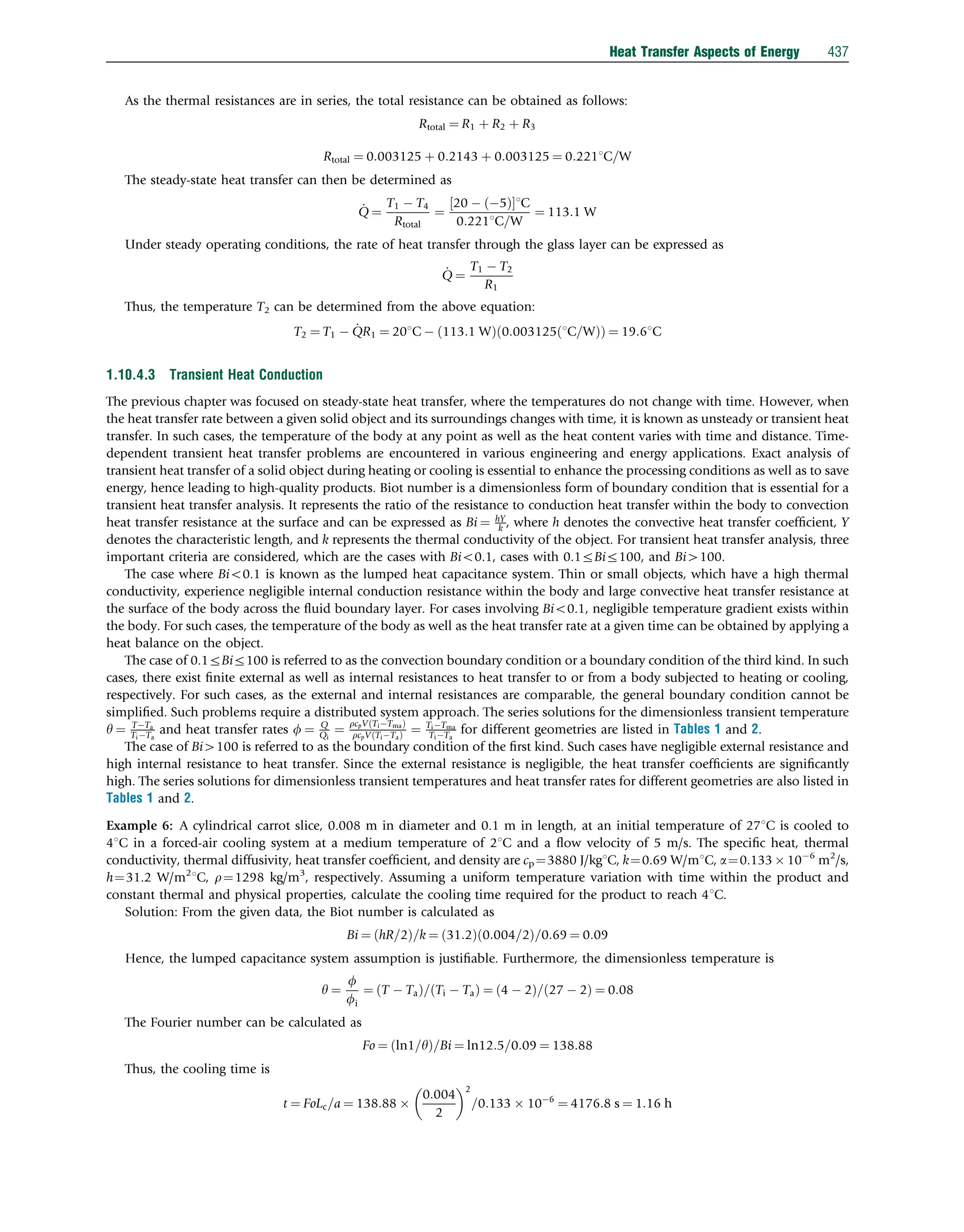
The results are shown in Fig. 14.
Example 8: An individual cylindrical eggplant was cooled until the center temperature of 221C reached 71C in the water pool of a
hydro cooling unit at a temperature of 11C. During the cooling process, the center temperature distribution of the product was
measured at 30-s intervals. Some physical and thermal properties of the product are: R¼0.0225 m, J¼0.142 m, k¼0.6064 W/m
1C, a¼1.438 107
m2
/s, and h¼44.15 W/m2
1C. Further information on the experiments and analysis technique, along with the
relevant data, can be found in Ref. [2]. Here, we will determine the theoretical center temperature distribution of the cylindrical
eggplant and compare it with the experimental data.
Table 1 Dimensionless transient temperatures
Equations or series solutions
For Bio0.1
y¼eBiFo
For 0.1rBir100
Infinite slab
y ¼
P
1
n ¼ 1
AnBnCn
An ¼ 1
ð Þnþ1
2Bi Bi2
þ m2
n
0:5
=mn Bi2
þ Bi þ m2
n
Bn ¼ exp m2
nFo
Cn ¼ cosmnG
Infinite cylinder
y ¼
P
1
n ¼ 1
AnBnCn
An ¼ 2Bi= m2
n þ Bi2
J0 mnR
ð Þ
Bn ¼ exp m2
nFo
Cn ¼ J0 mnG
ð Þ
Sphere
y ¼
P
1
n ¼ 1
AnBnCn An ¼ 1
ð Þnþ1
2Bi m2
n þ Bi 1
ð Þ2
h i0:5
= Bi2
Bi þ m2
n
Bn ¼ exp m2
nFo
Cn ¼ sinmnG=mnG
For Bi4100
Infinite slab
y ¼
P
1
n ¼ 1
AnBnCn
An ¼ 1
ð Þnþ1
2=mn
ð Þ
Bn ¼ exp m2
nFo
Cn ¼ cosmnG
mn ¼ 2n 1
ð Þp=2
Infinite cylinder
y ¼
P
1
n ¼ 1
AnBnCn
An ¼ 2=mnJ1 mn
ð Þ
Bn ¼ exp m2
nFo
Cn ¼ J0 mnG
ð Þ
J0 mnG
ð Þ ¼ 1 m2
n=22
þ m4
n=22
42
m6
n=22
42
62
Sphere
y ¼
P
1
n ¼ 1
AnBnCn
An ¼ 2 1
ð Þnþ1
Bn ¼ exp m2
nFo
Cn ¼ sinmnG=mnG
mn ¼ np
438 Heat Transfer Aspects of Energy

18. Solution: From the data we have, the Biot number can be calculated as
Bi ¼
hR
k
¼ 44:15 0:0225=0:6064 ¼ 1:64
Table 2 Transient heat transfer rates
Equations or series solutions
For Bio0.1
Qt ¼ Qi 1 exp BiFo
ð Þ
½
Qi ¼ rcpV Ti Ta
ð Þ
f ¼ Q
Qi
¼ TiTma
TiTa
For 0.1rBir100
Infinite slab
f ¼
P
1
n ¼ 1
AnBn
An ¼ 2Bi2
=m2
n Bi2
þ Bi þ m2
n
Bn ¼ 1 exp m2
nFo
Tma is the temperature at G¼0.57l
Infinite cylinder
f ¼
P
1
n ¼ 1
AnBn
An ¼ 4Bi2
=m2
n Bi2
þ m2
n
Bn ¼ 1 exp m2
nFo
Tma is the temperature at G¼0.7R
Sphere
f ¼
P
1
n ¼ 1
AnBn
An ¼ 6Bi2
=m2
n Bi2
þ m2
n Bi
Bn ¼ 1 exp m2
nFo
Tma is the temperature at G¼0.77R
For Bi4100
Infinite slab
f ¼
P
1
n ¼ 1
AnBn
An ¼ 2=m2
n ¼ 8= 2n 1
ð Þ2
p2
Bn ¼ 1 exp m2
nFo
Infinite cylinder
f ¼
P
1
n ¼ 1
AnBn
An ¼ 4=m2
n
Bn ¼ 1 exp m2
nFo
Sphere
f ¼
P
1
n ¼ 1
AnBn
An ¼ 6=m2
n ¼ 6=n2
p2
Bn ¼ 1 exp m2
nFo
1.0
0.8
0.6
0.4
0.2
Dimensionless
center
temperature
0.0
0 5 10
Fourier number
15 20
Computed
Experimental (1)
25 30
Fig. 14 Measured and predicted temperature distribution for an individual sample. Adapted from Dincer I. Analytical modelling of heat transfer
from a single slab in freezing. Int J Energy Res 1995;19(3):227–33.
Heat Transfer Aspects of Energy 439

19. Here, the Biot number is between 0.1rBir100, leading to a convection boundary condition problem. By knowing the Biot
number as 1.64, the values of mn and An for n¼1 6, which are considered sufficient terms, are taken as m1¼1.497, m2 ¼4.219,
m3 ¼7.242, m4 ¼10.332, m5 ¼13.445 and m6 ¼16.571 and A1 ¼1.297, A2 ¼ 0.427, A3¼0.203, A4 ¼ 0.119, A5 ¼0.0823, and
A6 ¼ 0.0589. The theoretical dimensionless center temperature is calculated from the following equation, considering Fo40.2:
yt ¼
X
1
n ¼ 1
AnBn ¼
X
6
n ¼ 1
Anexp m2
nFo
¼ 1:297 exp 1:4972
Fo
0:427 exp 4:2192
Fo
þ 0:203 exp 7:2422
Fo
0:119 exp 10:3322
Fo
þ 0:0823 exp 13:4452
Fo
0:0589 exp 16:5712
Fo
where Fo¼at/R2
¼1.438 107
t/0.02252
.
The computed results are shown in Fig. 15. The experimental results can also be obtained from Ref. [2].
Example 9: An individual spherical pear was cooled until the center temperature of 221C reached 21C in the water pool of a hydro
cooling unit at a temperature of 11C. During the cooling process, the center temperature distribution of the product was measured
at 30-s intervals. Some physical and thermal properties of the product are: R¼0.03 m, k¼0.5527 W/m 1C, a¼1.378 107
m2
/s,
and h¼160.56 W/m2
1C. Further information on the experiments, and analysis technique, along with the relevant data, can be
found in Ref. [2]. Here, we will determine the theoretical center temperature distribution of the spherical pear and compare it with
the experimental data.
Solution: From the data we have, the Biot number can be calculated as
Bi ¼
hR
k
¼ 160:56 0:030=0:5572 ¼ 8:64
Here, the Biot number is between 0.1rBir100, leading to a convection boundary condition problem. By knowing the Biot
number as 8.64, the values of mn and An for n¼1–6, which are considered sufficient terms, are taken as m1 ¼2.79, m2 ¼5.646,
m3 ¼8.581, m4 ¼11.578, m5 ¼14.618 and m6 ¼17.618 and A1 ¼1.903, A2 ¼ 1.657, A3¼ 1.42, A4 ¼ 1.196, A5 ¼1.018, and
A6 ¼ 0.878. The theoretical dimensionless center temperature is calculated from the following equation, considering Fo40.2:
yt ¼
X
1
n ¼ 1
AnBn ¼
X
6
n ¼ 1
Anexp m2
nFo
¼ 1:903 exp 2:792
Fo
1:675 exp 5:6462
Fo
þ 1:42exp 8:5812
Fo
1:196 exp 11:5782
Fo
þ 1:018 exp 14:6182
Fo
0:878 exp 17:6862
Fo
where Fo¼at/R2
¼1.378 107
t/0.032
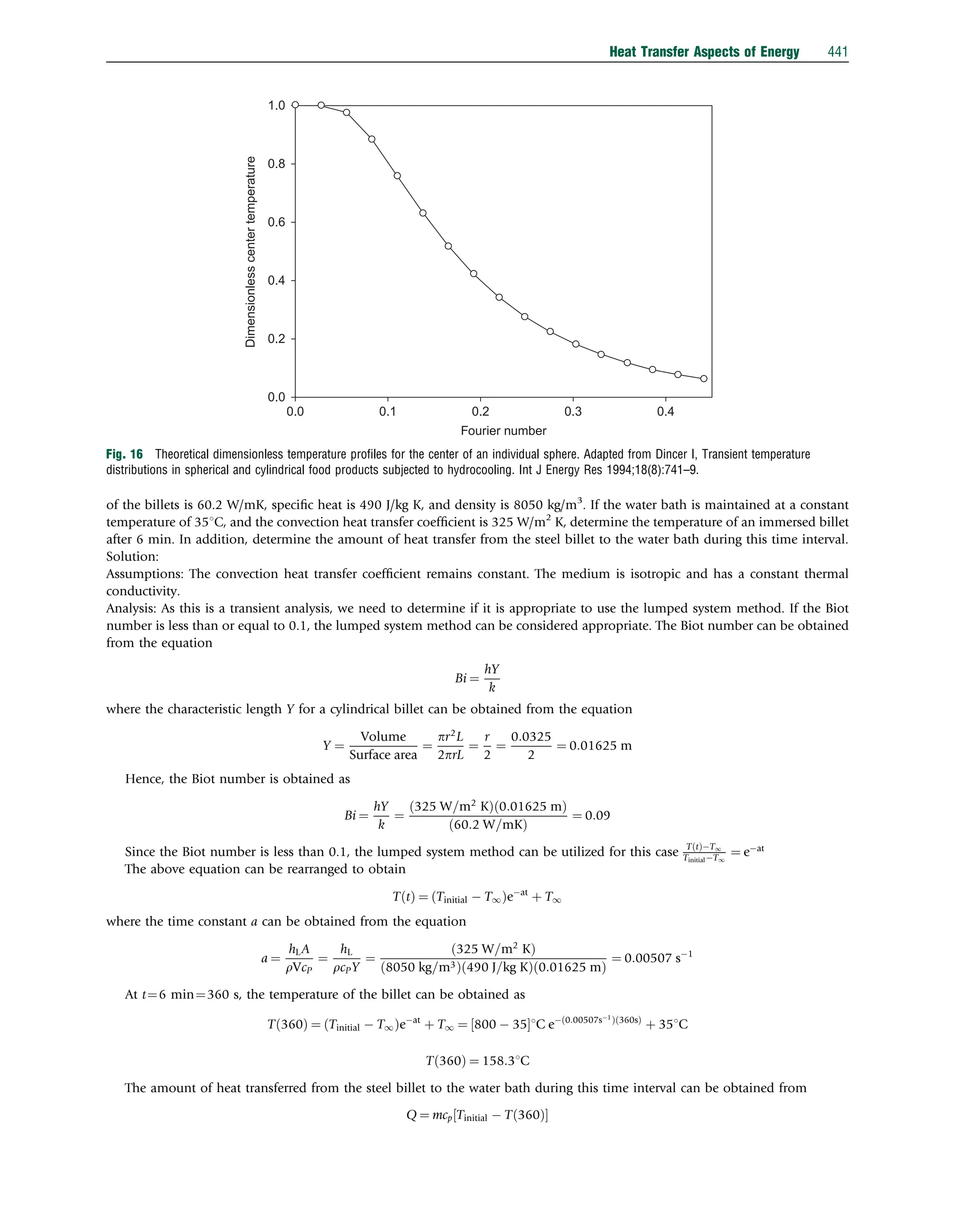
. The computed results are shown in Fig. 16, the experimental results can also be obtained
from Ref. [2].
Example 10: Steel billets are used extensively in the manufacturing of various products for numerous industries. The heat
treatment process of steel billets involves heating the billets to a temperature of 8001C and immersing them in a water bath until
they are cooled to a specified temperature. The billets have a diameter of 6.5 cm and a length of 100 cm. The thermal conductivity
1.0
0.8
0.6
0.4
Dimensionless
center
temperature
0.2
0.0 0.1 0.2
Fourier number
0.3 0.4 0.6
0.5 0.7
Fig. 15 Theoretical dimensionless temperature profiles for the center of an individual eggplant.
440 Heat Transfer Aspects of Energy

20. of the billets is 60.2 W/mK, specific heat is 490 J/kg K, and density is 8050 kg/m3
. If the water bath is maintained at a constant
temperature of 351C, and the convection heat transfer coefficient is 325 W/m2
K, determine the temperature of an immersed billet
after 6 min. In addition, determine the amount of heat transfer from the steel billet to the water bath during this time interval.
Solution:
Assumptions: The convection heat transfer coefficient remains constant. The medium is isotropic and has a constant thermal
conductivity.
Analysis: As this is a transient analysis, we need to determine if it is appropriate to use the lumped system method. If the Biot
number is less than or equal to 0.1, the lumped system method can be considered appropriate. The Biot number can be obtained
from the equation
Bi ¼
hY
k
where the characteristic length Y for a cylindrical billet can be obtained from the equation
Y ¼
Volume
Surface area
¼
pr2
L
2prL
¼
r
2
¼
0:0325
2
¼ 0:01625 m
Hence, the Biot number is obtained as
Bi ¼
hY
k
¼
325 W=m2
K
ð Þ 0:01625 m
ð Þ
60:2 W=mK
ð Þ
¼ 0:09
Since the Biot number is less than 0.1, the lumped system method can be utilized for this case T t
ð ÞT1
TinitialT1
¼ eat
The above equation can be rearranged to obtain
T t
ð Þ ¼ Tinitial T1
ð Þeat
þ T1
where the time constant a can be obtained from the equation
a ¼
hLA
rVcP
¼
hL
rcPY
¼
325 W=m2
K
ð Þ
8050 kg=m3
ð Þ 490 J=kg K
ð Þ 0:01625 m
ð Þ
¼ 0:00507 s1
At t¼6 min¼360 s, the temperature of the billet can be obtained as
T 360
ð Þ ¼ Tinitial T1
ð Þeat
þ T1 ¼ 800 35
½ 1C e 0:00507s1
ð Þ 360s
ð Þ
þ 351C
T 360
ð Þ ¼ 158:31C
The amount of heat transferred from the steel billet to the water bath during this time interval can be obtained from
Q ¼ mcp Tinitial T 360
ð Þ
½
1.0
0.8
0.6
0.4
0.2
Dimensionless
center
temperature
0.0
0.0 0.1 0.2
Fourier number
0.3 0.4
Fig. 16 Theoretical dimensionless temperature profiles for the center of an individual sphere. Adapted from Dincer I, Transient temperature
distributions in spherical and cylindrical food products subjected to hydrocooling. Int J Energy Res 1994;18(8):741–9.
Heat Transfer Aspects of Energy 441

21. where the mass of the billet can be obtained from the density and volume
m ¼ rV ¼ 8050 kg=m3
p 0:03252
m2
1 m
ð Þ
¼ 26:7 kg
Hence, Q ¼ 26:7 kg
ð Þ 490 J=kg K
ð Þ 800 158:3
ð Þ1C 8:4 MJ.
Example 11: A long steel shaft at 3001C cools in an environment at 351C. The heat transfer coefficient is calculated to be 60 W/m2
K. The thermal conductivity of the shaft is 15 W/mK, density is 8080 kg/m3
, specific heat is 490 J/kg K. If the shaft has a diameter of
25 cm, determine the temperature at its center and the amount of heat lost per unit length of the shaft after 1 h.
Solution:
Assumptions: As the shaft is specified to be long and contains a thermal symmetry about its centerline, heat transfer is considered
one-dimensional. The material is isotropic with constant thermal conductivity.
Analysis: In case of one-dimensional transient heat conduction, the temperature at the center of the shaft can be
approximated from the first term of the series solution if the Fourier number is greater than 0.2. The Fourier number can be
calculated as:
t ¼
at
r2
o
¼
kt
rcpr2
0
¼
15 W=mK
ð Þ 3600 s
ð Þ
8080 kg=m3
ð Þ 490 J=kg K
ð Þ 0:1252
m2
ð Þ
¼ 0:8740:2
Since the Fourier number is greater than 0.2, one term approximation can be used.
Bi ¼
hr0
k
¼
60 W=m2
K
ð Þ 0:125 m
ð Þ
15 W=m K
ð Þ
¼ 0:5
y0 ¼
T T1
Tinitial T1
¼
2
l1
J1 l1
ð Þ
J2
0 l1
ð Þ þ J2
1 l1
ð Þ
el2
1t
J0
l1r
r0
where l1 is the root of the eigenfunction l1
j1 l1
ð Þ
j0l1
¼ Bi ¼ 0:5
l1 ¼ 0:9408; J1 l1
ð Þ ¼ 0:4195; J0 l1
ð Þ ¼ 0:7902
Hence; y0 ¼
T0 T1
Tinitial T1
¼
2
0:9408
ð Þ
0:4195
0:79022
ð Þ þ 0:41952
ð Þ
e0:94082
0:87
ð Þ
0:7902
ð Þ ¼ 0:405
Therefore; T0 ¼ Tinitial T1
ð Þ 0:405
ð Þ þ T1 ¼ 300 35
ð Þ 0:405
ð Þ þ 35 ¼ 142:331C
The ratio of the amount of heat lost to the maximum amount of heat the shaft can lose is
Q
Qmaximum
¼ 1 2y0
J1 l1
ð Þ
l1
Hence; Q ¼ Qmaximum 1 2y0
J1 l1
ð Þ
l1
¼ Qmaximum 1
2 0:405
ð Þ 0:4195
ð Þ
0:9408
Q ¼ 0:639 Qmaximum ¼ 0:639rVcP T1 Tinitial
ð Þ ¼ 0:639 396:62 kg
ð Þ 490 J=kg K
ð Þ 35 300
½ 1C ¼ 32:9 MJ
Thus, 32.9 MJ of energy is lost per unit length of the shaft during this process.
1.10.5 Convection Heat Transfer
Convection mode of heat transfer takes place within a fluid when one portion of the fluid is mixed with another. Heat transfer by
convection can be classified according to the nature of the flow. Flows that are caused by external means such as a fan, pump, or
atmospheric wind are classified as forced convection. However, when the flow is induced due to buoyancy forces in the fluid
arising from density variations, which are caused by temperature differences within the fluid, it is classified as natural or free
convection. For instance, when a hot food item is exposed to the atmosphere, natural convection takes place; on the other hand,
for a food product placed in a cold store, forced-convection heat transfer occurs between the air flow and a food item, which is
subjected to this flow. When transfer of heat takes place through solid objects, the mode of heat transfer is conduction alone;
however, the transfer of heat from a solid surface to a liquid or gas occurs partly due to conduction and partly due to convection.
When an appreciable movement of the gas or liquid exists, the conduction heat transfer becomes negligibly small compared with
the heat transfer by convection in the gas or liquid. However, a thin boundary layer of fluid always exists on the surface, and
conduction heat transfer occurs through this thin film. When convection heat transfer occurs within a fluid, it is by combined
effects of conduction and bulk fluid motion. Generally, the transferred heat is the sensible heat of the fluid. In cases where a phase
change between the liquid and vapor states is taking place, the convection processes also include latent heat exchange.
442 Heat Transfer Aspects of Energy

22. 1.10.5.1 Newton’s Law of Cooling
The heat transfer that occurs between a solid surface and a fluid is proportional to the surface area and the temperature difference
between the fluid and the solid surface; this is known as Newton’s law of cooling. This represents a specific nature of convection
heat transfer and is expressed as
_
Q ¼ hA Ts Tf
ð Þ ð53Þ
where h represents the convection heat transfer coefficient. The heat transfer coefficient includes all effects influencing convection
heat transfer and it depends on the boundary layer conditions, which are dependent on factors such as the nature of the fluid flow,
thermal properties, surface geometry, and physical properties. The above equation does not take into account the heat transfer
due to radiation. Radiation heat transfer is discussed later. In many cases, the heat transfer due to radiation is negligibly small as
compared to conduction or convection heat transfer between a surface and a fluid. However, in heat transfer problems, which
involve in high surface temperatures and natural convection, radiation heat transfer is similar in magnitude to the natural
convection heat transfer.
Consider the wall in Fig. 17, heat transfer occurs from the higher temperature fluid A to the lower temperature fluid B through a
wall that has a thickness L. The temperature in fluid A drops to a temperature Ts1 within the wall region. Generally, the bulk fluid
temperature is nearly constant, apart from the thin films DA or DB near the surface of the wall. The rate of heat transfer per unit
surface area from the higher temperature fluid A to the wall and from the wall to the lower temperature fluid B are:
q ¼ hA TA Ts1
ð Þ ð54Þ
q ¼ hB Ts2 TB
ð Þ ð55Þ
In addition, the conduction heat transfer in the thin films can be expressed as
q ¼
kA
DA
TA Ts1
ð Þ ð56Þ
q ¼
kB
DB
Ts2 TB
ð Þ ð57Þ
Equating Eqs. (54–57), the convection heat transfer coefficients can be obtained as
hA ¼
kA
DA
and hB ¼
kB
DB
Hence, the rate of heat transfer per unit surface area in the wall can be obtained as
q ¼
k
L
Ts1 Ts2
ð Þ ð58Þ
In case of steady-state heat transfer, Eq. (54) is equal to Eq. (55) and thus to Eq. (58).
q ¼ hA TA Ts1
ð Þ ¼ hB Ts2 TB
ð Þ ¼
k
L
Ts1 Ts2
ð Þ ð59Þ
L
ΔB
ΔA
TB
TA
TS2
TS1
Fig. 17 A wall cross-section subject to convection heat transfer from both sides.
Heat Transfer Aspects of Energy 443

23. Therefore, Eq. (51) leads to the following expression
q ¼
TA TB
ð Þ
1
hA
þ L
k þ 1
hB
ð60Þ
An analogy between Eqs. (46) and (52) leads to the following expression
_
Q ¼ H A TA TB
ð Þ ð61Þ
where H represents the overall heat transfer coefficient and can be expressed as
1
H
¼
1
hA
þ
L
k
þ
1
hB
ð63Þ
Example 12: Consider a wall that has a height of 1 m, a width of 2 m, a thickness of 0.25 m, and a thermal conductivity of 1.2 W/
mK. The temperature of the room (TA) is measured to be 201C and the outside temperature (TB) is measured to be 51C, if the
convection heat transfer coefficients at the inner and outer surfaces of the window are hA ¼12 W/m2
K and hB¼35 W/m2
K,
determine the rate of heat loss from the room through this wall.
Solution:
Assumptions: Steady-state conditions persist. The heat transfer is considered one-dimensional. The medium is isotropic with
constant thermal conductivity.
Analysis: The rate of heat loss can be determined from the equation
_
Q ¼ HA TA TB
ð Þ
where the overall heat transfer coefficient H can be obtained as
1
H
1
hA
þ
L
k
þ
1
hB
¼
1
12
þ
0:25
1:2
þ
1
35
¼ 0:32 m2
K=W
Thus, H ¼ 1
1:78 ¼ 3:12 W=m2
K.
The inside and outside temperatures of the room are known, hence _
Q can be determined as
_
Q ¼ HA TA TB
ð Þ ¼ 3:12 W=m2
K
2m2
20 ð5Þ
½ 1C
_
Q ¼ 156:13 W
Thus, 156.13 J of heat is lost every second from the room through this wall.
Example 13: The double-pane window shown in Fig. 18, has a height of 1 m and a width of 2 m. The glass layers have a thickness
of 5 mm and a thermal conductivity of 0.80 W/mK. A 15-mm stagnant air space with a thermal conductivity of 0.035 W/mK
separates the two glass layers. The inner temperature of the room (Ti) is measured to be 231C and the outside temperature (To) is
measured to be 101C, if the convection heat transfer coefficient at the inner side of the wall is 12 W/m2
K and at the outer side of
the wall is 35 W/m2
K, determine the rate of heat loss from the room through this window.
Solution:
Assumptions: Steady-state conditions persist. The heat transfer is considered one-dimensional. The medium is assumed to be
isotropic with constant thermal conductivity (Fig. 19).
Analysis: The rate of heat loss through this window can be determined from the equation
_
Q ¼ HA Ti To
ð Þ
Glass
1 m
Air
Fig. 18 Double-pane window.
444 Heat Transfer Aspects of Energy

24. where H represents the overall heat transfer coefficient. In this case, H can be determined as
1
H
¼
1
hi
þ
Lglass
kglass
þ
Lair
kair
þ
Lglass
kglass
þ
1
ho
1
H
¼
1
12
þ
0:005
0:8
þ
0:015
0:035
þ
0:005
0:8
þ
1
35
¼ 0:55 m2
K=W
H ¼ 1:81 W=m2
K
Since the temperatures inside (Ti) and outside (To) of the room are known, _
Q can be obtained as
_
Q ¼ HA Ti To
ð Þ ¼ 1:81 W=m2
K
ð Þ 2 m2
ð Þ 23 10
ð Þ
½ 1C
_
Q ¼ 119:5 W
1.10.5.2 The Nusselt Number
In the analysis of convection heat transfer mechanism, the governing equations are commonly nondimensionalized by combining
the variables and grouping them into dimensionless numbers; this reduces the total number of variables. The heat transfer
coefficient h is nondimensionalized with the Nusselt number. The Nusselt number is defined as
Nu ¼
hY
kf
ð63Þ
where Y denotes the characteristic length and k denotes the fluid thermal conductivity. Nusselt number is also known as the
dimensionless convection heat transfer coefficient and is named after Wilhelm Nusselt. In the first half of the 20th century,
Wilhelm Nusselt contributed significantly to convective heat transfer.
Nusselt number essentially signifies the ratio of the convective heat transfer through a fluid layer of thickness Y, which has a
temperature T1 on one side of the fluid and temperature T2 on the other side during the presence of some fluid motion to the
conductive heat transfer through the fluid when the fluid layer is stagnant.
Nu ¼
_
qconvection
_
qconduction
¼
h T1 T2
ð Þ
kf T1T2
ð Þ
L
¼
hY
kf
ð64Þ
1.10.5.3 Forced Convection
The analysis of forced convection heat transfer deals with the heat transfer taking place between a solid surface and a moving fluid.
In order to apply the equation for Newton’s law of cooling as given in Eq. (1), it is required to determine the heat transfer
coefficient h. Nusselt–Reynolds correlations can be utilized for this purpose. The definition of Reynolds number as well as of the
Nusselt number is given in Table 3. A few examples of equipment involved in forced convection heat transfer include heat
exchangers, forced water and air coolers, forced water and air condensers, and evaporators.
Forced convection can occur in various types of cases, such as flow in or across a tube, and flow across a flat plate. These types of
cases can be solved mathematically with certain assumptions regarding the boundary conditions. Obtaining exact solutions to
T1
Ti
To
T2
T3
T4
Fig. 19 Heat transfer and temperature distribution through a double-pane window.
Heat Transfer Aspects of Energy 445

25. such cases can be extremely difficult, particularly for cases that involve in turbulent flows; however, approximate solutions can be
obtained by making appropriate assumptions.
The first step in obtaining a solution of a convective heat transfer problem is to determine whether the boundary layer is
turbulent or laminar. The value of the convective heat transfer coefficient h and thus the rate of convective heat transfer are affected
by these conditions.
Fluid motion within the laminar boundary layer is highly ordered, and streamlines along which the particles move can be
identified. In contrast, in the turbulent boundary layer, fluid motion is highly irregular and it is characterized by the fluctuations in
velocity that start to develop in the transitional region; after the transitional boundary layer, a complete turbulent boundary layer
exists. These velocity fluctuations increase the transfer of heat, momentum, and species, and thus increase the surface friction and
rates of convective heat transfer. In addition, the laminar sublayer is approximately linear, and the transport is primarily domi-
nated by diffusion as well as the velocity profile. Furthermore, there exists an adjoining buffer layer in which turbulent mixing and
diffusion are comparable. However, transport in the turbulent region is mainly dominated by turbulent mixing.
The value of the Reynolds number at which the transition from laminar to turbulent occurs is known as the critical Reynolds
number. The critical Reynolds number is dependent on the geometry as well as flow conditions.
1.10.5.3.1 External flow forced convection
When a fluid flow is not confined to a specific channel or passage, and flows unboundedly over any surface such as a pipe, flat
plate, cylinder, or sphere, it is classified as external flow. In order to determine the heat transfer rates for external flow cases, several
correlations between the dimensionless parameters Nusselt number, Reynolds number, and Prandtl number are utilized. These
correlations were developed based on experimental data. The fluid properties required to obtain these dimensionless parameters
are usually taken at the film temperature Tfm. The film temperature is an average of the fluid free stream and surface temperatures
Tfm ¼ TsþTa
2 . The various forced convection heat transfer correlations for external flow for different geometries, with the pertinent
parameters listed in Table 4.
Example 14: The top cover of a horizontal solar flat plate collector is at a temperature of 501C. The solar collector is located at a
location where the wind speed and temperature are determined to be 8.3 m/s and 221C. The length and width of the top cover are
3 m and 1 m, respectively.
1. Determine the rate of convective heat loss from the cover in these conditions.
2. Analyze the effect on the rate of convective heat loss from the cover as the air velocity varies from 5 to 10 m/s while other
parameters remain constant.
3. Analyze the effect on the rate of convective heat loss from the cover as the air temperature varies from 5 to 351C while other
parameters remain constant.
Solution:
Schematic (Fig. 20):
Assumptions: Steady-state operating conditions persist.
Analysis:
1. The rate of heat loss from the top cover of a horizontal solar flat plate collector is to be determined; the fluid in this case is air.
The properties of air required to obtain the dimensionless parameters should be evaluated at the film temperature Tfm.
Tfm ¼
Ts þ Ta
2
¼
50 þ 22
½ 1C
2
¼ 361C
At 361C, density of air r is 1.14 kg/m3
, Prandtl number Pr is 0.71, the kinematic viscosity n is 1.66 105
m2
/s, and the thermal
conductivity is 0.0276 W/mK.
Table 3 List of important heat transfer dimensionless parameters
Name Symbol Definition Application
Biot number Bi hY/k Steady- and unsteady-state conduction
Fourier number Fo at/Y2
Unsteady-state conduction
Graetz number Gz GY2
cp/k Laminar convection
Grashof number Gr gbDTY3
/n2
Natural convection
Rayleigh number Ra Gr Pr Natural convection
Nusselt number Nu hY/kf Natural or forced convection, boiling, or condensation
Peclet number Pe UY/a¼Re Pr Forced convection (for small Pr)
Prandtl number Pr cpm/k¼n/a Natural or forced convection, boiling, or condensation
Reynolds number Re UY/n Forced convection
Stanton number St h/rUcp ¼Nu/Re Pr Forced convection
446 Heat Transfer Aspects of Energy

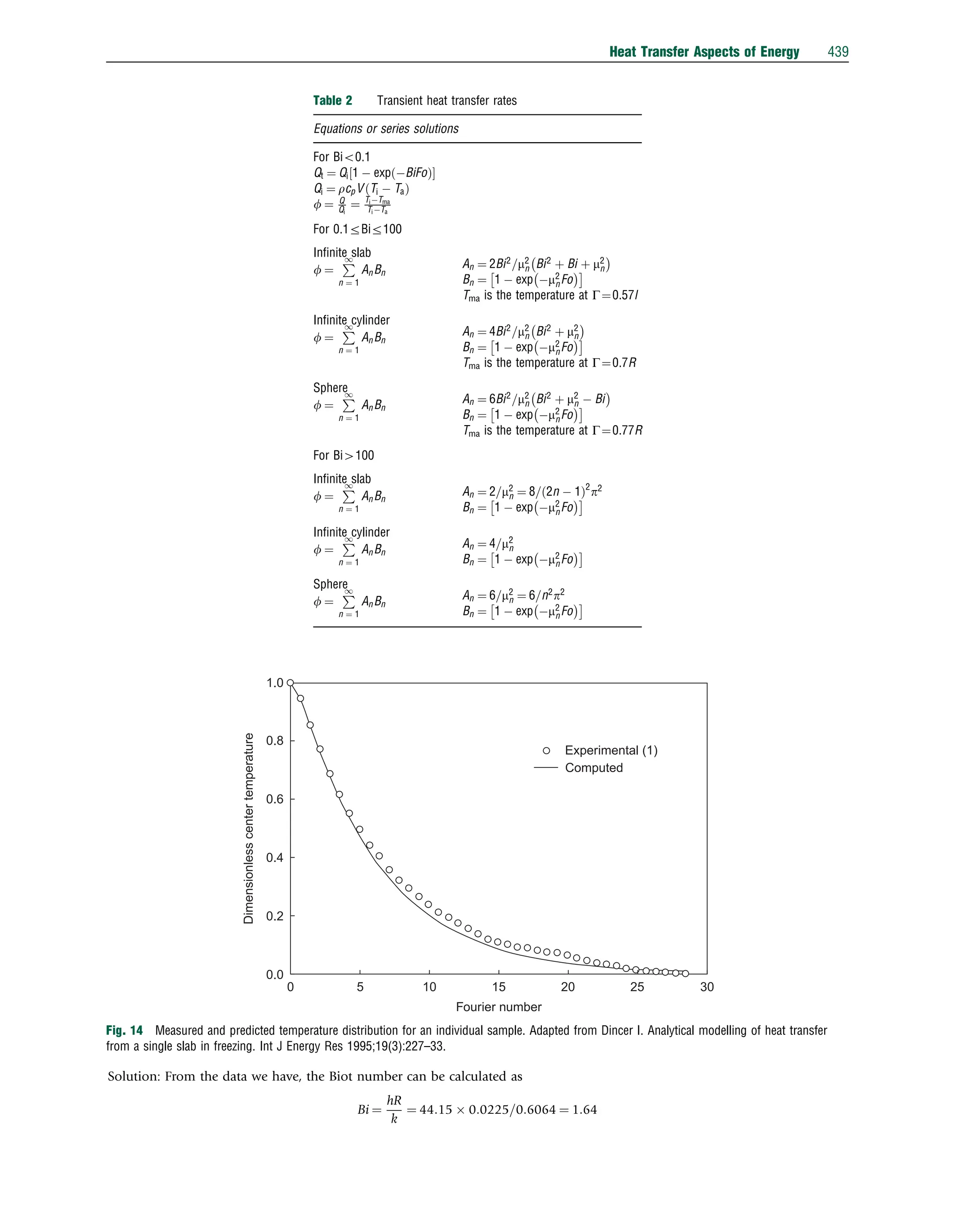
26. The Reynolds number at the plate end can be determined as follows:
Re ¼
UY
v
¼
8:3 m=s
ð Þ 3m
ð Þ
ð1:66 105
Þm2=s
¼ 15 105
45 105
Since the Reynolds number is greater than the critical Reynolds number, a suitable correlation to be used for this case is
Nu ¼ 0:037Re
4
5 871
Pr
1
3 ¼ 0:037 15 105
4
5
871
0:71
1
3 ¼ 2097
Table 4 Forced convection heat transfer correlations and equations
Equation or correlation
Correlations for external flow over a flat plate
Nu¼0.332Re1/2
Pr1/3
for PrZ0.6 for laminar; local; Tfm
Nu¼0.664Re1/2
Pr1/3
for PrZ0.6 for laminar; average; Tfm
Nu¼0.565Re1/2
Pr1/2
for Prr0.05 for laminar; local; Tfm
Nu¼0.0296Re4/5
Pr1/3
for 0.6rPrr60 for turbulent; local; Tfm, Rer108
Nu¼(0.037Re4/5
871)Pr1/3
for 0.6oPro60 for mixed flow; average; Tfm, Rer108
Correlations for external cross-flow over circular cylinders
Nu¼cRen
Pr1/3
for PrZ0.7 for average; Tfm; 0.4oReo4 106
where
c¼0.989 and n¼0.330 for 0.4oReo4
c¼0.911 and n¼0.385 for 4oReo40
c¼0.683 and n¼0.466 for 40oReo4000
c¼0.193 and n¼0.618 for 4000oReo40,000
c¼0.027 and n¼0.805 for 40,000oReo400,000
Nu¼cRen
Prs
(Pra/Prs)1/4
for 0.7oPro500 for average; Ta; 1oReo106
where
c¼0.750 and n¼0.4 for 1oReo40
c¼0.510 and n¼0.5 for 40oReo1000
c¼0.260 and n¼0.6 for 103
oReo2 105
c¼0.076 and n¼0.7 for 2 105
oReo106
s¼0.37 for Prr10
s¼0.36 for Pr410
Nu¼0.3 þ [(0.62Re1/2
Pr1/3
)/(1 þ (0.4/Pr)2/3
)1/4
][1 þ (Re/28,200)5/8
]4/5
for RePr40.2 for average; Tfm
Correlations for internal flow in tubes
Nu¼4.36 for constant surface heat flux; fully developed; laminar
Nu¼3.66 for constant surface temperature; fully developed; laminar
Nu¼3.66 þ (0.065(D/L) Re Pr)/(1 þ 0.04[(D/L) Re Pr)]2/3
for constant surface temperature; developing flow; laminar
Nu¼0.023Re4/5
Prn
for 0.7rPrr160; turbulent; fully developed; ReZ10,000; n¼0.4 for fluid heating; n¼0.3 for fluid
cooling
Nu¼4.8 þ 0.0156Re0.85
Prs
0.93
for liquid metal flow; constant surface temperature; 104
oReo106
Nu¼6.3 þ 0.0167Re0.85
Prs
0.93
for liquid metal flow; constant surface heat flux; 104
oReo106
Correlations for external cross-flow over spheres
Nu/Pr1/3
¼0.37Re0.6
/Pr1/3
for average; Tfm; 17oReo70,000
Nu¼2 þ (0.4Re1/2
þ 0.06Re2/3
)Pr0.4
(ma/ms)1/4
for 0.71oPro380
for average; Ta; 3.5oReo7.6 104
; 1o(ma/ms)o3.2.
Correlation for falling drop
Nu¼2 þ 0.6Re1/2
Pr1/3
[25(x/D)0.7
] for average; Ta
Source: Reproduced from Dincer I. Heat transfer in food cooling applications. Washington, DC: Taylor Francis; 1997.
Air
Ta = 22°C
U = 8.3 m s−1
3m
Ts = 50°C
Fig. 20 Heat transfer from a flat plate solar collector.
Heat Transfer Aspects of Energy 447

27. Once the Nusselt number is determined, the heat transfer coefficient h can be obtained from the equation
Nu ¼
hY
k
h ¼ Nu
k
Y
¼ 2097
0:0276 W=mK
3 m
¼ 18:92 W=m2
K
Hence, the rate of heat loss from the collector cover can be determined as
_
Q ¼ hA Ts Tf
¼ 18:92 W=m2
K
3 m 1 m
ð Þ 50 22
½ 1C ¼ 1589 W
2. The effect of changing air velocity U on the rate of convective heat loss from the cover while all other parameters are held
constant is shown in Fig. 21. As can be depicted from the graph, at 10 m/s the rate of heat loss increases to 1939 W, while at 5
m/s, it drops to 863.7 W.
3. The effect of varying air temperature Ta on the rate of convective heat loss from the cover while all other parameters are held
constant is shown in Fig. 22. As can be depicted from the graph, as the air temperature rises to 351C, the rate of heat loss drops
to 832 W, whereas at an air temperature of 51C, the rate of heat loss rises to 2635 W.
Example 15: In various energy applications, the excess energy available during a process is stored in a medium for later use.
Thermal energy storage involves storing the excess produced energy in the form of thermal energy. Consider a cylindrical thermal
energy storage tank of diameter 3 m and a height of 5 m. The efficiency of a thermal energy storage decreases as the thermal losses
from the tank increase. Assume the temperature of the outer surface of the thermal energy storage tank remains constant at 501C.
1. Determine rate of convective heat loss from the tank if the local wind speed is 2 m/s and temperature is 221C.
2. Analyze the effect of changing air temperature on the rate of heat loss from the tank.
3. If the overall energy efficiency of a closed thermal energy storage system is defined as
Zoverall ¼
Energy recovered
Energy input
Determine the overall energy efficiency for a day for the conditions given above if the total energy input was 24 GJ and analyze
the effect of air temperature on the overall efficiency.
Solution:
Assumptions: Steady-state operating conditions persist. The external surface temperature of the tank remains uniform and
constant.
1. The external surface temperature of the tank is assumed to be constant at 501C. The velocity of cross-flow wind and temperature
are also known. The properties of air need to be determined at film temperature Tfm. The film temperature can be evaluated as
Tfm ¼
Ts þ Ta
ð Þ
2
¼
50 þ 22
½ 1C
2
¼ 361C
5.0 5.5 6.0 6.5 7.0 7.5 8.0 8.5 9.0 9.5 10.0
800
900
1000
1100
1200
1300
1400
1500
1600
1700
1800
1900
2000
2100
U (m s−1)
Q
loss
(W)
Fig. 21 Effect of air velocity on convective heat loss.
448 Heat Transfer Aspects of Energy

28. At this temperature, density (r) of air is 1.1 kg/m3
, the kinematic viscosity (n) is 1.66 105
m2
/s, Prandtl number (Pr) is 0.71,
and the thermal conductivity (k) is 0.027 W/mK.
After obtaining the properties, the Reynolds number can be determined from the equation
Re ¼
UY
v
For cases involving external cross flow over a cylinder, the diameter represents the characteristic length Y. Hence, the Reynolds
number is calculated as
Re ¼
UY
v
¼
2 m=s
ð Þ 3 m
ð Þ
1:66 105
m2=s
ð Þ
¼ 361; 445:8
Based on the Reynolds number, the suitable correlation can be chosen from Table 2:
Nu ¼ 0:027Re0:805
Pr
1
3 ¼ 0:027 361; 445:780:805
0:71
1
3
¼ 717:8
From the Nusselt number, the convective heat transfer coefficient h can be obtained as
h ¼ Nu
k
Y
¼ 717:8
ð Þ
0:027 W=mK
ð Þ
ð3 mÞ
¼ 6:5 W=m2
K
After obtaining the convective heat transfer coefficient, the Newton’s law of cooling can be applied to determine the rate of
convective heat loss from the tank:
_
Q ¼ hA Ts Ta
ð Þ ¼ 6:5 W=m2
K
p 3 m
ð Þ 5 m
ð Þ 50 22
½ 1C ¼ 8576:5 W
2. The effect of air temperature on the rate of heat loss is shown in Fig. 23. As the air temperature decreases to 101C, the rate
of heat loss increases to 18,859 W. However, when the air temperature reaches 351C, then the rate of heat loss decreases
to 4507 W.
3. The overall energy efficiency of the storage tank can be expressed as
Zoverall ¼
Energy recovered
Energy input
¼
Qrecovered
Qin
¼ 1
QL
Qch
where QL denotes the energy lost and Qch represents the energy input to the tank during charging. Hence, the overall efficiency can
be determined as
Zoverall ¼ 1
8576 24 3600 J
ð Þ
24 109
J
ð Þ
¼ 0:97
Hence, the overall efficiency of the storage tank is 97% assuming the temperature of the tank and other given conditions remain
constant.
5 10 15 20 25 30 35
1000
1250
1500
1750
2000
2250
2500
Ta (°C)
Q
loss
(W)
Fig. 22 Effect of ambient temperature on convective heat loss.
Heat Transfer Aspects of Energy 449

29. The effect of air temperature on the overall efficiency is shown in Fig. 24. The efficiency drops to 93% at an air temperature of
101C and increases to 98.4% at a temperature of 351C.
Example 16: Condensers are used extensively in refrigeration cycles to extract heat from the working fluid. Consider a section of a
circular cylindrical condenser pipe that has an external surface temperature of 651C. Air at a velocity of 15 m/s is passes over the
pipe. The pipe has a length of 2 m and a diameter of 15 cm. If the temperature of air passing over the pipe is 181C,
1. Determine the rate of heat loss from the surface of the pipe due to convection.
2. Analyze the effect of changing the air velocity from 5 to 35 m/s on the convective heat transfer rate.
Solution:
Assumptions: Steady-state operating conditions persist. The external surface temperature of the pipe remains uniform and
constant.
Analysis:
1. The outer surface temperature of the condenser is known. Also, the cross-flow air velocity and temperature are also known.
To determine the dimensionless parameters required, properties of air at the film temperature Tfm are necessary. The film
−10 −5 0 5 10 15 20 25 30 35
0
2000
4000
6000
8000
10,000
12,000
14,000
16,000
18,000
20,000
Ta (°C)
Q
loss
(W)
Fig. 23 Effect of ambient temperature on heat loss rate.
−10 −5 0 5 10 15 20 25 30 35
0.93
0.935
0.94
0.945
0.95
0.955
0.96
0.965
0.97
0.975
0.98
0.985
Ta (°C)
overall
Fig. 24 Effect of ambient temperature on overall efficiency.
450 Heat Transfer Aspects of Energy

30. temperature can be evaluated as
Tfm ¼
Ts þ Ta
ð Þ
2
¼
65 þ 18
½ 1C
2
¼ 41:51C
At this temperature, density (r) of air is 1.1 kg/m3
, the kinematic viscosity (n) is 1.72 105
m2
/s, Prandtl number (Pr) is 0.71,
and the thermal conductivity (k) is 0.027 W/mK.
The Reynolds number can be determined from Re ¼ UY
v where Y represents the characteristic length. For the case of external cross
flow over a cylinder, the characteristic length is represented by its diameter. Hence, the Reynolds number is calculated as
Re ¼
UY
v
¼
15 m=s
ð Þ 0:15 m
ð Þ
1:72 10 5 m2=s
ð Þ
¼ 130; 814
Based on the Reynolds number, the suitable correlation can be chosen from Table 2
Nu ¼ 0:027Re0:805
Pr
1
3 ¼ 0:027 130; 8140:805
0:71
1
3
¼ 316:7
After determining the Nusselt number, the convective heat transfer coefficient h can be obtained as
h ¼ Nu
k
Y
¼ 316:7
ð Þ
0:027 W=mK
ð Þ
ð0:15 mÞ
¼ 57 W=m2
K
Once the convective heat transfer coefficient is determined, the Newton’s law of cooling can be applied
_
Q ¼ hA Ts Ta
ð Þ ¼ 57 W=m2
K
p 0:15 m
ð Þ 2 m
ð Þ 65 18
½ 1C ¼ 2524:9 W
2. The effect of increasing or decreasing air velocity on the convective heat transfer rate is depicted in Fig. 25. As can be observed,
the rate of heat transfer increases considerably as the air velocity increases. At a velocity of 35 m/s, the rate of convective heat
transfer is 5083 W. However, at a velocity of 5 m/s, the rate of heat transfer drops to 1061 W.
Example 17: It is essential to measure the temperature of the combustion gases produced in the combustion chamber of a power
plant. A thermocouple that has a spherical junction of 0.85 mm diameter is inserted in a passage in which the combustion gases
flow with a velocity of 3.5 m/s. The thermal conductivity of the junction is 80 W/mK, density is 8575 kg/m3
, and specific heat is
410 J/kg K. Whereas, the combustion gases are estimated to have a thermal conductivity of 0.075 W/mK, a kinematic viscosity of
39 106
m2
/s, and a Prandtl number of 0.71.
1. When the thermocouple is inserted in the passage, its temperature rises and the temperature difference between the thermo-
couple junction and combustion gases decreases. Determine the time required by the thermocouple for the temperature
difference to reach 5% of its initial value.
2. Analyze how the response time of the thermocouple changes as the specific heat of the spherical junction is varied while other
parameters remain constant.
3. Analyze the effect of changing velocity of combustion gases and changing thermal conductivity of the junction on the time
required by the thermocouple for the temperature difference to reach 5% of its initial value.
5 10 15 20 25 30 35
1600
2400
3200
4000
4800
5600
U (m s−1
)
Q
(W)
Fig. 25 Effect of air velocity on heat loss rate.
Heat Transfer Aspects of Energy 451

31. Solution:
Assumptions:
1. The combustion gases have a constant temperature. Radiation heat transfer is negligible.
Analysis: This case involves changing of temperature with time. If the Biot number is less than 0.1, the lumped system method can
be utilized.
Bi ¼
hY
k
where the characteristic length Y for a sphere can be obtained from the equation
Y ¼
Volume
Surface area
¼
4
3
pr3
4pr2
¼
r
3
¼
0:000425
3
¼ 0:00014 m
In order to determine the heat transfer coefficient h, the Nusselt number is required. The appropriate correlation for the Nusselt
number can be chosen from Table 2. For the case of external cross-flow over spheres, the suitable correlation is
Nu ¼ 2 þ 0:4Re
1
2 þ 0:06Re
2
3
Pr0:4 ma
ms
1
4
where the Reynolds number can be calculated as
Re ¼
UY
v
¼
3:5 m=s
ð Þ 0:00085 m
ð Þ
39 106
m2=s
ð Þ
¼ 76:3
Substituting the Reynolds number in the Nusselt number correlation
Nu ¼ 2 þ 0:4 76:3
ð Þ
1
2 þ 0:06 76:3
ð Þ
2
3
0:710:4
¼ 5:98
Once the Nusselt number is obtained, the heat transfer coefficient can be determined
h ¼ Nu
k
D
¼ 5:98
0:075 W=m K
ð Þ
0:00085 m
ð Þ
¼ 527:65 W=m2
K
The Biot number can then be obtained as
Bi ¼
hY
k
527:65 W=m2
K
ð Þ 0:00014 m
ð Þ
80 W=mK
ð Þ
¼ 9:2 104
Since the Biot number is less than 0.1, the lumped system method can be utilized. The time required by the thermocouple to reach
5% of the initial temperature difference can be calculated by the lumped system method as
t ¼
rVcp
hA
ln
Ti Ta
T Ta
¼
rcpr
3h
ln
Ti Ta
0:05 Ti Ta
ð Þ
¼
8575 kg=m3
ð Þ 410 J=kg K
ð Þ 0:000425 m
ð Þ
3
ð Þ 527:65 W=m2 K
ð Þ
ln 20
ð Þ
t ¼ 2:83 s
Hence, it will take approximately 2.83 s for the thermocouple junction to reach 5% of the initial temperature difference.
2. The effect of changing specific heat on the response time of the thermocouple is shown in Fig. 26; as can be observed, the
response increases to 5.5 s at a specific heat value of 800 J/kg K and drops to 0.7 s at a specific heat value of 100 J/kg K.
3. The effect of changing velocity of combustion gases from 2 to 35 m/s on the thermocouple time to reach 5% of initial
temperature difference is shown in Fig. 27. As can be depicted from the figure, the response time of the thermocouple drops
significantly as the velocity increases. At a velocity of 35 m/s, the response time decreases to 1.1 s; whereas, at a low velocity of
2 m/s, the response time increases to 3.4 s.
Example 18: In a heat exchanger, hot water at 951C flows through the tubes of a tube bank. The tubes are arranged as shown in
Fig. 28 and have an outer diameter of 1 cm. Air at a mean velocity of 6 m/s enters the tube bank and flows in a normal direction
over the tubes. The tube bank contains 20 rows of tubes and 10 tubes in each row. If air enters the tube bank with a temperature of
181C, determine the outlet temperature. Also, determine rate of heat transfer that occurs between the flowing air and tubes per unit
length of tubes. In addition, analyze how the air exit temperature and the rate of heat transfer changes with the number of rows of
tubes in the tube bank.
Solution:
Assumptions: Steady operation conditions persist. The temperature of hot water flowing through the tubes is equal to the outer
surface temperature of the tubes.
Analysis: The initial step in such analysis involves determining the properties of the fluid at the mean temperature, which in this
case is air. However, since the exit temperature of air is unknown, an initial mean temperature value of 251C is taken to determine
452 Heat Transfer Aspects of Energy

32. 100 200 300 400 500 600 700 800
0
0.5
1.0
1.5
2.0
2.5
3.0
3.5
4.0
4.5
5.0
5.5
t
(s)
cp (J/kgK)
Fig. 26 Effect of specific heat on response time.
2 5 8 11 14 17 20 23 26 29 32 35
0.5
1.0
1.5
2.0
2.5
3.0
3.5
U (m s−1)
t
(s)
Fig. 27 Effect of combustion gases velocity on thermocouple response time.
3 cm
3 cm
Air
V = 6 m s−1
T = 18°C
Fig. 28 Cooling of water in a tube bank.
Heat Transfer Aspects of Energy 453

33. the required properties. After obtaining the final result, this value will be compared to the obtained value. The density of air at
251C and atmospheric pressure is 1.18 kg/m3
, Prandtl number at 251C is 0.7073 and at a surface temperature is 0.7006, kinematic
viscosity 1.55 105
m2
/s, specific heat is 1006 J/kg K and thermal conductivity is 0.026 W/mK.
In cases involving tube banks, Reynolds number is evaluated at the maximum velocity, which occurs while the fluid flows
within the tube bank. The maximum velocity can be calculated from the distances between the tubes given in the figure as
Vmaximum ¼ dt
dt D V, where dt denotes the distance between the tubes in the transverse direction, V represents the approaching
velocity, and D represents the diameter of the tubes.
Vmaximum ¼
dt
dt D
V ¼
0:03 m
0:03 0:01
ð Þm
6 m=s
ð Þ ¼ 9 m=s
Re ¼
VmaximumD
v
¼
9 m=s
ð Þ 0:01 m
ð Þ
1:55 105
m2=s
ð Þ
¼ 5806:5
Based on the Reynolds number, the applicable Nusselt number correlation can be utilized:
Nu ¼ 0:27Re0:63
Pr0:36 Pr
Prs
0:25
¼ 0:27 5806:50:63
0:70730:36
0:7073
0:7006
0:25
¼ 56:2
Once the Nusselt number is determined, heat transfer coefficient h can be obtained as
h ¼
Nu k
D
¼
56:2 0:026 W=mK
ð Þ
0:01 m
¼ 146:1 W=m2
K
There are 20 rows with 10 tubes in each row, hence, there are 200 tubes in total. The surface area per unit length of tube
subjected to heat transfer can be calculated as
A ¼ npDL ¼ 200p 0:01 m
ð Þ 1 m
ð Þ ¼ 6:28 m2
The mass flow rate of air can be calculated as
_
ma ¼ rV 10 0:03 m
ð Þ 1 m
ð Þ
ð Þ ¼ 1:18 kg=m3
6 m=s
ð Þ 0:3 m2
¼ 2:124 kg=s
The exit temperature of air can be determined from the equation
Te ¼ Ts Ts Ti
ð Þexp
hA
_
macp
¼ 95 95 18
ð Þexp
146:1 W=m2
K
ð Þ 6:28 m2
ð Þ
2:124 kg=s
ð Þ
_
1006 J=m2 K
ð Þ
!
Te ¼ 44:91C
Hence, the air exits the tube bank of the heat exchanger at a temperature of 44.91C.
The rate of heat transfer per unit length of the tubes can be determined from the equation
_
Q ¼ _
mcp Te Ti
ð Þ ¼ 2:124 kg=s
ð Þ 1006 J=kg K
ð Þ 44:9 18
½ 1C ¼ 57:5 103
W ¼ 57:5 kW
The mean temperature assumed was 251C, whereas the mean temperature from the obtained results is
TiþTe
ð Þ
2 ¼ 18þ44:9
2 ¼ 31:451C. When the above calculations are repeated with a mean temperature of 31.451C, a _
Q value of 57.23 kW
is obtained.
The effect on the air exit temperature and heat transfer rate as the number of rows of tubes changes is shown in Fig. 29. As can
be observed from the figure, the heat transfer rate increases to 88 kW when the 36 rows of tubes are used, while the exit
temperature increases to 601C (Figs. 29 and 30).
1.10.5.3.2 Internal flow forced convection
When a fluid flow is restricted to flow within a given passage such as pipe or duct, it is classified as internal flow. Internal flow forced
convection cases are encountered in various energy applications. Heat gain or loss by the air flowing in the ducts of air conditioning
systems is an example of internal flow forced convection. In addition, heat loss from steam pipes in a power plant is also a typical
example. In internal flow cases, as the fluid flow is restricted within a pipe or duct, the boundary layer has a limit unto which it can
grow. In order to determine the heat transfer rates, correlations between dimensionless parameters such as Nusselt number,
Reynolds number, and Prandtl number are utilized. Pertinent correlations for different types of cases have been listed in Table 2.
The correlations can be used to determine the Nusselt number and thus the heat transfer coefficient for a given case.
Example 19: A boiler utilizes hot air to generate steam. The hot air flows through a 3-meter-long tube passing through the boiler.
Consider a case in which the water in the boiler is being boiled at a temperature of 1051C. Air enters the 10-cm-diameter tube at a
temperature of 2801C and flows with an average velocity of 5 m/s. If the temperature of the tube at its outer surface is equal to the
temperature of the boiling water, determine
1. The convective heat transfer coefficient of the air flowing in the tubes.
2. Rate of steam generation in the boiler.
454 Heat Transfer Aspects of Energy

34. Solution:
Assumptions:
• Steady-state operation conditions persist.
• The outer temperature of the tube is equal to the temperature of the boiling water in the boiler.
• Negligible pipe thermal resistance.
• Tube inner surface is smooth.
Analysis:
1. The exit temperature of air is not known, hence, the properties of air are obtained at an assumed mean temperature of 2001C.
After obtaining the exit temperature, the calculations will be repeated with the obtained new mean temperature. The density of
air is 0.73 kg/m3
, Prandtl number is 0.69, specific heat is 1026 J/kg K, thermal conductivity is 0.039 W/mK, and kinematic
viscosity is 3.59 105
.
The average velocity of air through the tube is known to be 5 m/s, so the Reynolds number can be calculated:
Re ¼
VD
v
¼
5 m=s
ð Þ 0:1 m
ð Þ
3:59 105
m2=s
ð Þ
13; 927:6
16 20 24 28 32 36
40
45
50
55
60
Number of rows
T
e
(°C)
Fig. 29 Effect of number of rows on air exit temperature.
16 20 24 28 32 36
40
50
60
70
80
90
100
Number of rows
Q
(kW)
Fig. 30 Effect of number of rows on the heat transfer rate.
Heat Transfer Aspects of Energy 455

35. The Reynolds number is greater than 10,000, hence the flow is turbulent, assuming the flow is fully developed throughout the
tube. The appropriate Nusselt number correlation is chosen from Table 2.
Nu ¼ 0:023Re0:8
Pr0:3
¼ 0:023 13; 927:6
ð Þ0:8
0:69
ð Þ0:3
¼ 42:5
Thus, the convective heat transfer coefficient h is obtained from the equation
h ¼ Nu
k
D
¼ 42:5
0:039 W=m K
ð Þ
ð0:1 mÞ
¼ 16:6 W=m2
K
2. The temperature of air at the exit of the tube can be obtained as
Te ¼ Ts Ts Ti
ð Þexp
hA
_
mcp
¼ 1051C
ð Þ 105 280
½ 1C exp
16:6 W=m2
K
ð Þ p 0:1 m
ð Þ 3 m
ð Þ
ð Þ
0:029 kg=s
ð Þ 1026 J=kg K
ð Þ
Te ¼ 210:61C
In case of internal flow constant surface temperature, the logarithmic mean temperature difference is calculated as
DTlm ¼
Te Ti
ð Þ
ln TsTe
TsTi
¼
257:3 280
½ 1C
ln 105275:3
105280
¼ 137:41C
For internal flow constant surface temperature cases, the rate of convective heat transfer can be obtained from the equation
_
Q ¼ hADTlm ¼ 16:6 W=m2
K
p 0:1 m
ð Þ 3 m
ð Þ
ð Þ 137:41C
ð Þ ¼ 2083 W
Once the rate of heat transfer is obtained, the rate of steam generation in the boiler can be determined
_
msteam ¼
_
Q
hfg
¼
2556:3 W
2; 257; 000 J=kg
¼ 0:00092 kg=s
The properties of air were determined at an initial assumed mean temperature of 2001C. Evaluating the air properties at the
new mean temperature T ¼ 210:6þ280
2 ¼ 245:31C
, and repeating the above calculations, we obtain Te ¼2091C; _
Q¼1962 W
_
msteam ¼ 0:00087 kg=s.
Example 20: During the design of an air conditioning system, the heat loss from a duct while operating in the heating mode of
operation is being considered. The duct has a square cross-section of dimensions 0.3 m 0.3 m and has a length of 10 m (Fig. 31).
The temperature of air as it enters the duct is measured to be 651C. The temperature of the duct remains nearly constant at 401C. If
air flows through the duct at an average velocity of 4 m/s, determine the rate at which heat is lost from the air as it travels through
the duct.
Solution:
Assumptions: Steady-state operation conditions persist. The duct inner surface is smooth. And the temperature of the duct remains
constant.
Analysis: The exit temperature of air is not known; hence, the bulk fluid mean temperature cannot be determined. The properties
of air are determined at the inlet temperature of 651C. After obtaining the outlet temperature, the calculations will be repeated with
the obtained mean temperature. At 651C, the density of air is 1.044 kg/m3
, specific heat is 1008 J/kg K, thermal conductivity is
0.029 W/mK, kinematic viscosity is 1.9 105
m2
/s, and Prandtl number of 0.7.
As the duct is noncircular, the hydraulic diameter needs to be determined to evaluate the Reynolds number. The hydraulic
diameter Dh is obtained as
Dh ¼
4Acs
p
¼
4 0:3 m 0:3 m
ð Þ
ð4 0:3 mÞ
¼ 0:3 m
Air
65°C
Ts = 40°C
L = 10 m
Fig. 31 Heat loss from a duct.
456 Heat Transfer Aspects of Energy

36. The Reynolds number can then be calculated using the hydraulic diameter
Re ¼
VDh
v
¼
4 m=s
ð Þ 0:3 m
ð Þ
1:9 105
m2=s
ð Þ
¼ 63157:9
Since the Reynolds number is greater than 10,000, the flow is turbulent. The entry lengths are approximately equal to 10Dh¼3 m.
As the length of the duct is much longer than the entry lengths, the flow can be assumed to be fully developed throughout the duct.
To obtain the Nusselt number, the appropriate correlation for the case of fully developed turbulent internal flow can be applied
Nu ¼ 0:023Re0:8
Pr0:3
¼ 0:023 63157:90:8
0:70:3
¼ 143:1
The heat transfer coefficient can be determined from the Nusselt number and the hydraulic diameter
h ¼ Nu
k
Dh
143:1
0:029 W=m K
ð Þ
ð0:3 mÞ
¼ 13:8 W=m2
K
After obtaining the heat transfer coefficient, the exit temperature of air can be determined
Te ¼ Ts Ts Ti
ð Þexp
hA
_
mcp
¼ 401C
½ 40 65
½ 1C exp
13:8 W=m2
K
ð Þ 4 0:3 m
ð Þ 10 m
ð Þ
ð Þ
0:38 kg=s
ð Þ 1008 J=kg K
ð Þ
Te ¼ 56:221C
As this is a case of constant surface temperature, the logarithmic mean temperature difference is calculated
DTlm ¼
Ti Te
ð Þ
ln TsTe
TsTi
¼
65 56:22
½ 1C
ln 4056:22
4065
¼ 20:31C
The rate of heat loss from the duct can be obtained as
_
Q ¼ hADTlm ¼ 13:8 W=m2
K
4 0:3 m 10 m
ð Þ 20:31C
ð Þ ¼ 3361:7 W
The rate of heat loss from the duct is obtained to be 3361.7 W. After repeating the above calculations at the new mean
temperature of T ¼ 65þ56:22
2 ¼ 60:611C, the rate of heat loss is obtained as 3391 W.
Example 21: A solar thermal power plant utilizes parabolic trough solar collectors. The temperature of the concentrator fluid
as it leaves the solar collector is required to be 3901C, while it enters the solar collector at a temperature of 2901C. The heat
flux concentrated on the tube by the concentrator is approximated to be 18,500 W/m2
. The concentrator fluid has density of
850 kg/m3
, thermal conductivity of 0.09 W/mK, specific heat of 3000 J/kg K and a kinematic viscosity of 1.9 107
m2
/s. If the
fluid flows through a single tube with a mass flow rate of 3.2 kg/s,
1. Determine the length of the concentrator required if the tube has a diameter of 10 cm.
2. Plot the fluid temperature and surface temperature of the tube as a function of the collector length.
3. Analyze the effect of tube diameter on the required collector length.
Solution:
Assumptions: Steady operation conditions persist. The tube is thin walled. In addition, the heat flux on the tube surface is constant
and uniform.
Analysis:
1. The collector tube has a constant surface heat flux of 18,500 W/m2
, the inlet temperature of the concentrator fluid is known,
and the required tube length is to be determined to achieve the outlet temperature required.
Applying an energy balance on the tube
qA ¼ _
mcp To Ti
ð Þ
q pDL
ð Þ ¼ _
mcp To Ti
ð Þ
L ¼
_
mcp To Ti
ð Þ
q pD
ð Þ
¼
3:2 kg=s
ð Þ 3000 J=kg K
ð Þ 390 290
½ 1C
18; 500 W=m2
ð Þ p 0:1 m
ð Þ
ð Þ
¼ 165:2 m
The rate of heat transfer with this length of collector is
_
Q ¼ q pDL
ð Þ ¼ 18; 500 W=m2
p 0:1 m
ð Þ 165:2 m
ð Þ
ð Þ ¼ 9; 60; 133 W
2. The surface temperature of the tube can be determined from Newton’s law of cooling
q ¼ h Ts Tf
ð Þ
Heat Transfer Aspects of Energy 457

37. where h denotes the convective heat transfer coefficient, and Ts and Tf denote the surface and fluid temperatures
respectively.
Ts ¼
q
h
þ Tf
The Reynolds number can be determined as
Re ¼
4 _
m
pDm
¼
4 3:2 kg=s
ð Þ
p 0:1 m
ð Þ 1:62 104
Ns=m2
ð Þ
¼ 251; 504
Thus, the flow through the tube is turbulent. Assuming fully developed conditions exist, the Nusselt number correlation is
chosen from Table 2:
Nu ¼ 0:023Re
4
5Pr0:4
where the Prandtl number can obtained as
Pr ¼
mcp
k
¼
1:62 104
Ns=m2
ð Þ 3000 J=kg K
ð Þ
0:09 W=mK
ð Þ
¼ 5:4
After obtaining the Prandtl number, the Nusselt number can be obtained as
Nu ¼ 0:023 251; 504
4
5
5:40:4
¼ 944:3
The average heat transfer coefficient can be determined from the equation
h ¼ Nu
k
D
¼ 944:3
0:09 W=mK
0:1 m
¼ 849:9 W=m2
K
The fluid temperature in the tube as function of collector length l can be expressed as
Tf ðlÞ ¼ Ti þ
q pDl
ð Þ
_
mcp
Thus, the heat transfer coefficient h and fluid temperature Tf can substituted in the equation Ts ¼ q
h þ Tf to obtain the surface
temperature as a function of collector length l. The variation of the surface and fluid temperature with collector length is
depicted in Fig. 32. As can be observed from the graph, the surface temperature of tube is 3111C and 4111C at the inlet and exit
of the tube, respectively.
3. The effect of tube diameter on the required collector length is depicted in Fig. 33. If the diameter of the tube is reduced to 5 cm,
the collector length required to meet the outlet temperature of 3901C is 330 m, whereas, if the diameter is increased to 25 cm,
the required collector length decreases significantly to 66 m.
1.10.5.4 Natural Convection
Heat transfer by natural convection occurs due to variations in density arising from temperature differences. In many cases, the rate
of convective heat transfer due to natural convection is negligibly small. Natural convection heat transfer coefficients are generally
much smaller than forced convection heat transfer coefficients. In the absence of a forced fluid velocity, heat transfer occurs entirely
0 40 80 120 160
260
280
300
320
340
360
380
400
420
440
Collector length (m)
T
f
,
T
s
(°C)
Ts
Tf
Fig. 32 Effect of collector length on the surface and fluid temperature.
458 Heat Transfer Aspects of Energy

38. by natural convection in case of negligible radiation heat transfer. However, in some practical cases, the radiative effect is also
important to consider. Natural convection cases are encountered in various applications; for instance, in gravity coils, which are
used in high-humidity cold rooms as well as in roof-mounted condensers. In addition, such cases are also observed in condensers
and evaporators of domestic refrigerators as well as in baseboard radiators and convectors for space heating. In various systems,
which involve more than a single mode of heat transfer, the resistance to heat transfer due to natural convection is largest and thus
plays a significant role in the performance or design of a system. Furthermore, when heat transfer rates or the operating costs are to
be minimized, natural convection is preferable over forced convection.
Heat transfer due to natural convection is primarily influenced by gravitational force from thermal expansion, thermal dif-
fusion, and viscous drag. For this reason, natural convection is directly affected by the gravitational acceleration, thermal diffu-
sivity, kinematic viscosity, and coefficient of volume expansion. Correlations between Nusselt number, Prandtl number, and
Rayleigh number are generally used for natural convection cases.
The boundary layers in natural convection are not limited to laminar flow. As depicted in Fig. 34, there exists a transition from
laminar to turbulent flow in many cases.
The transition, which occurs in a natural convection boundary layer, depends on the relative magnitude of viscous and
buoyancy forces in the fluid. Its occurrence is generally correlated in terms of the Rayleigh number. For instance, the critical
Rayleigh number for vertical plates is approximately 109
. Similar to cases involving forced convection, a transition to turbulence
significantly affects the heat transfer.
Various natural convection heat transfer correlations for several cases of plates, cylinders, wires, pipes, etc. as well as heat
transfer coefficients are listed in Table 5. In cases involving natural convection heat transfer, calculate the Rayleigh number to
determine whether the boundary layer is turbulent or laminar. According to the boundary layer, the appropriate correlation for a
given case can be chosen from Table 3 to determine the heat transfer coefficient.
0.05 0.10 0.15 0.20 0.25
60
120
180
240
300
360
D (m)
L
(m)
Fig. 33 Effect of tube diameter on the required collector length.
Turbulent
Transition
Laminar
x
y
Quiescent
fluid
Ts T∞
Ts
T∞, g
Fig. 34 Natural convection on a vertical plate.
Heat Transfer Aspects of Energy 459

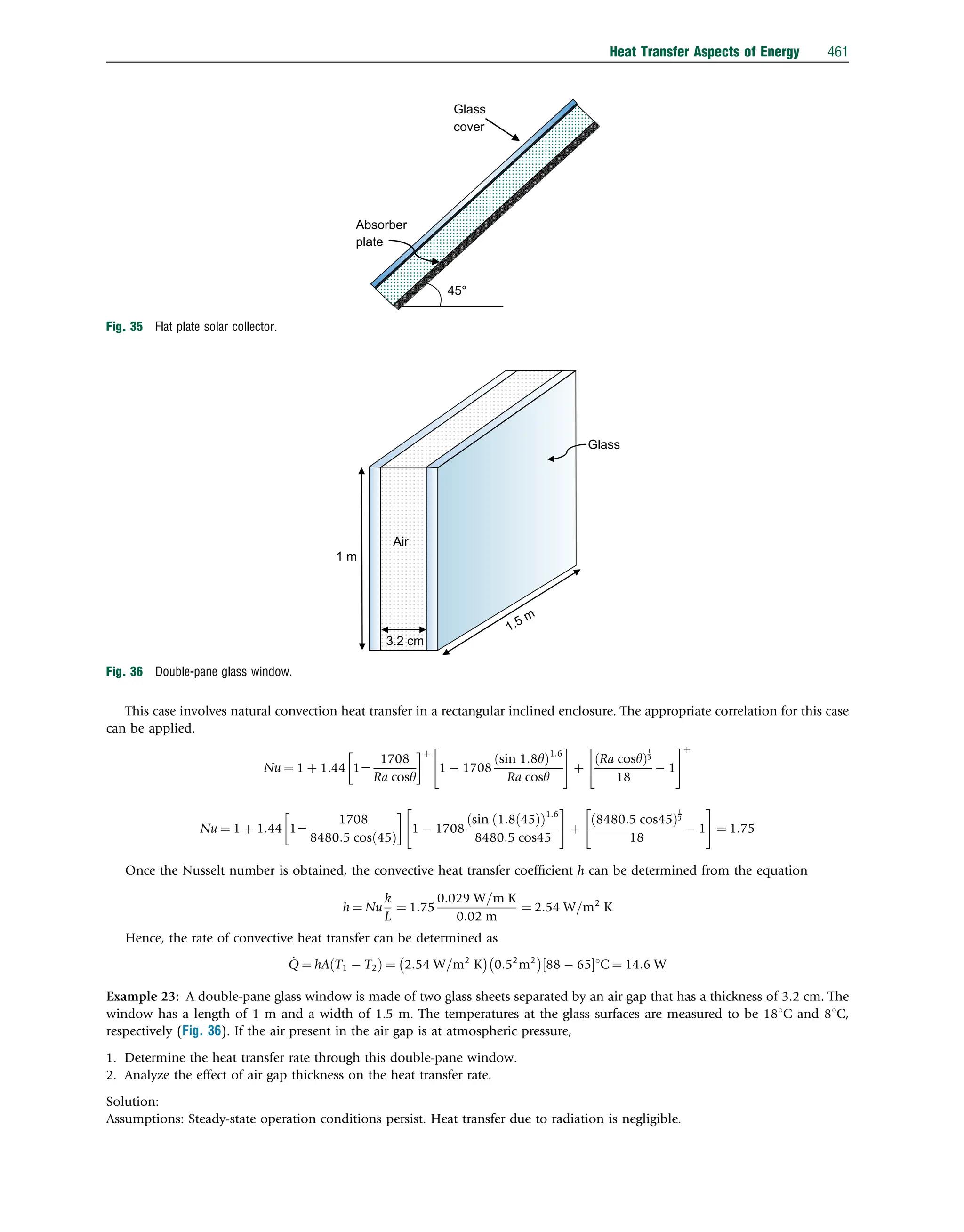
39. Example 22: Consider a flat plate solar collector. The collector is placed with a tilt angle of 45 degree and has dimensions
0.5 m 0.5 m. The absorber plate and the glass cover are positioned 2 cm apart. If the temperatures of the glass cover and the
absorber plate are measured to be 651C and 881C, respectively, determine the rate of heat loss due to natural convection from the
absorber plate of the collector (Fig. 35).
Solution: The mean temperature can be obtained as Tm ¼ 65þ88
½ 1C
2 ¼ 76:51C. The properties of air are obtained at this mean
temperature. The thermal conductivity k is 0:029 W=m2
K, kinematic viscosity n is 2.1 105
m2
/s, thermal diffusivity a is
2.9 105
m2
/s, and coefficient of volume expansion b is 1
273þ76:5
½ K ¼ 0:0029.
After obtaining the properties, the Rayleigh number can be determined
Ra ¼
gbDTL3
va
¼
9:81 m=s2
ð Þ 0:0029 1=K
ð Þ 231C
ð Þ 0:021m
ð Þ3
2:1 105
m2=s
ð Þ 2:9 105
m2=s
ð Þ
¼ 8480:5
Table 5 Natural convection heat transfer equations and correlations
Equation or correlation
General equations
Nu¼hY/kf ¼cRan
and Ra¼Gr Pr¼gb(Ts Ta)Y3
/na
where n is 1/4 for laminar flow and 1/3 for turbulent flow. Y is height for vertical plates or pipes, diameter for horizontal pipes and
spheres Tfm(Ts þ Ta)/2
Correlations for vertical plates (or inclined plates, inclined up to 60 degree)
Nu¼[0.825 þ 0.387Ra1/6
/(1 þ (0.492/Pr)9/16
)4/9
]2
for an entire range of Ra
Nu¼0.68 þ 0.67Ra1/4
/(1 þ (0.492/Pr)9/16
)4/9
for 0oRao109
Correlations for horizontal plates (YAs/P)
For upper surface of heated plate or lower surface of cooled plate:
Nu¼0.54Ra1/4
for 104
rRar107
Nu¼0.15Ra1/3
for 107
rRar1011
For lower surface of heated plate or upper surface of cooled plate:
Nu¼0.27Ra1/4
for 105
rRar1010
Correlations for horizontal cylinders
Nu¼hD/k¼cRan
where
c¼0.675 and n¼0.058 for 1010
oRao102
c¼1.020 and n¼0.148 for 102
oRao102
c¼0.850 and n¼0.188 for 102
oRao104
c¼0.480 and n¼0.250 for 104
oRao107
c¼0.125 and n¼0.333 for 107
oRao1012
Nu¼[0.60 þ 0.387Ra1/6
/(1 þ (0.559/Pr)9/16
)8/27
]2
for an entire range of Ra
Correlations for spheres
Nu¼2 þ [0.589Ra1/4
/(1 þ (0.469/Pr)9/16
)4/9
] for PrZ0.7 and Rar1011
Correlations for enclosures
Rectangular inclined enclosures
Nu¼1 þ 1.44[1–(1708/Ra cosy)]þ
(1 1708 (sin 1.8y)1.6
/Ra cosy) þ [(Ra cosy)1/3
/18) 1]þ
Vertical rectangular enclosures
Nu¼0.18[Ra (Pr/(0.2 þ Pr))]0.29
for 1oH/Lo2; RaPr/(0.2 þ Pr)4103
Nu¼0.22[Ra (Pr/(0.2 þ Pr))]0.28
(H/L) 1/4
for 2oH/Lo10; Rao1010
Nu¼0.42Ra1/4
Pr0.012
(H/L) 0.3
for 10oH/Lo40; 1oPro2 104
; 104
oRao107
Nu¼0.046Ra1/3
for 1oH/Lo40; 1oPro20; 106
oRao109
Concentric cylinders
keff/k¼0.386(Pr/(0.861 þ Pr))1/4
(Fc Ra)1/4
Heat transfer correlations
Gr Pr¼1.6 106
Y3
(DT)
where Y in m; DT in 1C
h¼0.29 (DT/Y)1/4
for vertical small plates in laminar range
h¼0.19 (DT)1/3
for vertical large plates in turbulent range
h¼0.27 (DT/Y)1/4
for horizontal small plates in laminar range (facing upward when heated or downward when cooled)
h¼0.22 (DT)1/3
for vertical large plates in turbulent range (facing downward when heated or upward when cooled)
h¼0.27 (DT/Y)1/4
for small cylinders in laminar range
h¼0.18 (DT)1/3
for large cylinders in turbulent range
Source: Reproduced from Dincer I. Heat transfer in food cooling applications. Washington, DC: Taylor Francis; 1997.
460 Heat Transfer Aspects of Energy

40. This case involves natural convection heat transfer in a rectangular inclined enclosure. The appropriate correlation for this case
can be applied.
Nu ¼ 1 þ 1:44 12
1708
Ra cosy
þ
1 1708
sin 1:8y
ð Þ1:6
Ra cosy
#
þ
Ra cosy
ð Þ
1
3
18
1
#þ
Nu ¼ 1 þ 1:44 12
1708
8480:5 cosð45Þ
1 1708
sin ð1:8ð45Þ
ð Þ1:6
8480:5 cos45
#
þ
8480:5 cos45
ð Þ
1
3
18
1
#
¼ 1:75
Once the Nusselt number is obtained, the convective heat transfer coefficient h can be determined from the equation
h ¼ Nu
k
L
¼ 1:75
0:029 W=m K
0:02 m
¼ 2:54 W=m2
K
Hence, the rate of convective heat transfer can be determined as
_
Q ¼ hA T1 T2
ð Þ ¼ 2:54 W=m2
K
0:52
m2
88 65
½ 1C ¼ 14:6 W
Example 23: A double-pane glass window is made of two glass sheets separated by an air gap that has a thickness of 3.2 cm. The
window has a length of 1 m and a width of 1.5 m. The temperatures at the glass surfaces are measured to be 181C and 81C,
respectively (Fig. 36). If the air present in the air gap is at atmospheric pressure,
1. Determine the heat transfer rate through this double-pane window.
2. Analyze the effect of air gap thickness on the heat transfer rate.
Solution:
Assumptions: Steady-state operation conditions persist. Heat transfer due to radiation is negligible.
45°
Absorber
plate
Glass
cover
Fig. 35 Flat plate solar collector.
Air
3.2 cm
1.5 m
1 m
Glass
Fig. 36 Double-pane glass window.
Heat Transfer Aspects of Energy 461

41. Analysis:
1. In this case, heat transfer between the two panes of the window occurs due to natural convection. Properties of air are obtained
at the mean temperature T ¼ T1þT2
2 ¼ 18þ8
½ 1C
2 ¼ 131C. At this temperature and atmospheric pressure, the kinematic viscosity of
air n is 1.4 10 5 m2
/s, the thermal conductivity k is 0.025 W/mK, the coefficient of volume expansion b is 1
13þ273
½ K ¼ 0:0035,
the thermal diffusivity a is 2.04 105
m2
/s.
The Rayleigh number can be determined from the equation
Ra ¼
gbDTL3
va
¼
9:81 m=s2
ð Þ 0:0035 1=K
ð Þ 101C
ð Þ 0:032 m
ð Þ3
1:4 105
m2=s
ð Þ 2:04 105
m2=s
ð Þ
¼ 39393:9
For cases involving vertical rectangular enclosures, the aspect ratio needs to be determined. The aspect ratio for the given
geometry can be calculated as H
L ¼ 1
0:032 ¼ 31:25. Based on the aspect ratio, Prandtl number and Rayleigh number, the
appropriate correlation can be chosen from Table 3
Nu ¼ 0:42Ra
1
4Pr0:012 H
L
0:3
¼ 0:42 39393:9
1
4
0:710:012
31:250:3
¼ 2:1
Once the Nusselt number is calculated, the heat transfer coefficient h can be obtained from the equation
h ¼ Nu
k
L
¼ 2:1
0:025 W=m2
K
0:032 m
¼ 1:64 W=m2
K
Hence, the rate of heat transfer through the double-pane window can be obtained as
_
Q ¼ hA T1 T2
ð Þ ¼ 1:64 W=m2
K
1 m 1:5 m
ð Þ 18 8
½ 1C ¼ 24:6 W
2. The effect of air gap thickness on the natural convective heat transfer rate is shown in Fig. 37. As can be observed, the
heat transfer rate increases with increasing air gap thickness. At an air gap thickness of 15 cm, the heat transfer rate increases to
26.7 W, whereas for 0.5-cm-thick air gap, the rate of heat transfer decreases to 22.5 W.
Example 24: A 32-meter-long pipe is used in a power plant to transport steam. Without insulation, the temperature at the outer
surface of the pipe is measured to be 1251C, whereas, the temperature of the surroundings is measured to be 251C. If the pipe has a
diameter of 8.2 cm (Fig. 38),
1. Determine the rate of heat loss from the pipe due to natural convection.
2. Analyze the effect of pipe diameter and surface temperature on the rate of heat loss from the pipe.
Solution:
Assumptions: Steady-state operation conditions persist. Radiation heat transfer is negligible.
Analysis:
1. The outer surface temperature of the pipe and surrounding air temperature is known. Properties of air are determined at the
atmospheric pressure and film temperature Tfm ¼ 125þ25
½ 1C
2 ¼ 751C. The thermal conductivity k is 0.029 W/mK, kinematic
0 1 2 3 4 5 6 7 8 9 10 11 12 13 14 15
22
23
24
25
26
27
Air gap thickness (cm)
Q
(W)
Fig. 37 Effect of air gap thickness on natural convective heat transfer.
462 Heat Transfer Aspects of Energy

42. viscosity n is 2.05 105
m2
/s, Prandtl number is 0.7, coefficient of volume expansion b is 0.0029, and the thermal diffusivity a
is 2.92 105
m2
/s.
With the obtained air properties at the film temperature, the Rayleigh number can be calculated
Ra ¼
gbDTD3
va
¼
9:81 m=s2
ð Þ 0:0029 1=K
ð Þ 1001C
ð Þ 0:082 m
ð Þ3
2:05 105
m2=s
ð Þ 2:92 105
m2=s
ð Þ
¼ 2:6 106
To obtain the Nusselt number, the appropriate correlation can be chosen from Table 3
Nu ¼ 0:6 þ
0:387Ra
1
6
1 þ 0:559
Pr
9
16
h i8
27
0
B
@
1
C
A
2
¼ 0:6 þ
0:387 2:6 106
ð Þ
1
6
1 þ 0:559
0:7
9
16
h i8
27
0
B
@
1
C
A
2
¼ 19:04
After calculating the Nusselt number, the heat transfer coefficient h can be obtained from the equation
h ¼ Nu
k
D
¼ 19:04
ð Þ
0:029 W=m K
0:082 m
¼ 6:73 W=m2
K
The outer surface area of the pipe can be calculated as A ¼ pDL ¼ pð0:082 mÞð32 mÞ ¼ 8:24 m2
.
The rate of heat loss from the pipe due to natural convection can be obtained as
_
Q ¼ hA TS T
ð Þ ¼ 6:73 W=m2
K
8:24 m2
125 25
½ 1C ¼ 5545:5 W
2. The effect of pipe diameter and surface temperature on heat loss rate is shown in Figs. 39 and 40. As it can be observed from the
graphs, the heat loss rate significantly increases with increasing pipe diameter and surface temperature. At a diameter of 20 cm,
the heat loss rate increases to 12,600 W, whereas, for a pipe diameter of 1 cm, the heat loss rate is 1100 W. If the surface
temperature of the pipe increases to 2001C, the heat loss rate increases to 11,765 W, whereas if the surface temperature drops to
1001C, the heat loss rate decreases to 3949 W.
Steam
32 m
Ts = 125°C
Fig. 38 Flow of steam through cylindrical pipe.
0 5 10 15 20
0
1500
3000
4500
6000
7500
9000
10,500
12,000
13,500
Pipe diameter (cm)
Q
loss
(W)
Fig. 39 Effect of pipe diameter on heat loss rate.
Heat Transfer Aspects of Energy 463

43. 1.10.5.5 Boiling Heat Transfer
Boiling is a phenomenon that occurs at a solid–liquid interface, when a liquid comes in contact with a surface that has a
temperature higher than its saturation temperature. If the temperature of the liquid at a certain pressure increases to the saturation
temperature, it starts to boil. Boiling is also considered to be a form of convective heat transfer, as a fluid motion is involved.
However, unlike other convection methods, boiling depends also on the latent heat of vaporization of a fluid as well as the
amount of surface tension at the vapor–liquid interface. During a constant pressure phase change process, the temperature remains
constant during the process under equilibrium conditions. The heat transfer coefficient for a heat transfer process during boiling is
generally higher than those cases involving in a single-phase convective heat transfer. The rate of heat transfer per unit area during
boiling from a given surface to the fluid can be expressed in the form of Newton’s law of cooling
_
qboil ¼ hboil Ts Tsat
ð Þ ð65Þ
where Ts and Tsat represent the surface and fluid saturation temperatures, respectively, and hboil represents the heat transfer
coefficient.
When boiling occurs in the absence of any bulk fluid flow, it is known as pool boiling; whereas, when boiling occurs during a
bulk fluid flow, it is called flow boiling. In pool boiling, natural convection currents or motion of bubbles may cause fluid motion
within the stationary fluid body. However, in cases involving in flow boiling, the fluid motion is generally caused by
external means.
A further classification of pool and flow boiling is saturated boiling or subcooled boiling. When the boiling process occurs at
the saturation temperature of the fluid, it is known as saturated boiling. Whereas, if the boiling process takes place when the bulk
liquid temperature is lower than the saturation temperature of the fluid, it is called subcooled boiling.
1.10.5.5.1 Pool boiling
In the process of pool boiling, the fluid motion is not caused by an external means such as a pump. Any motion that occurs in the
fluid is caused by natural convection currents as well as the motion of bubbles that are influenced by buoyancy forces. Different
regimes exist in a pool boiling process depending on the excess temperature (Ts Tsat). The first regime is known as natural
convection boiling, which occurs when the temperature of the fluid is slightly over the saturation temperature. The transfer of heat
from the surface to the fluid in this regime occurs by natural convection. If the excess temperature is increased further, the phase of
nucleate boiling initiates and bubbles start forming; this point is known the onset of nucleate boiling. As the excess temperature
increases further from this point, the rate of bubble formation and the heat flux rate increase up to a maximum point known as the
critical heat flux. Beyond this point, the heat flux rate decreases with increasing temperature difference up to certain point. This
region is known as transition boiling. The heat flux rate decreases in this region due to the surface being covered by a film of vapor
that acts an insulation layer. In the transition region, both nucleate and film boiling exist. However, as the excess temperature is
increased further, nucleate boiling is replaced completely by film boiling at a certain point. At this point, the heat flux rate reaches a
minimum value referred to as the minimum heat flux, after which it starts to increase with increasing excess temperature. This
region is referred to as film boiling. In this region, the heating surface is covered completely by a vapor film and the rate of heat flux
increases with increasing excess temperature due to radiation heat transfer that occurs between the high-temperature heating
surface and the fluid through the vapor film.
100 110 120 130 140 150 160 170 180 190 200
4000
5000
6000
7000
8000
9000
10,000
11,000
12,000
Q
loss
(W)
Ts (°C)
Fig. 40 Effect of surface temperature on heat loss rate.
464 Heat Transfer Aspects of Energy

44. As pool boiling comprises of these different regions, heat transfer relations according to the region need to be utilized
to determine the heat transfer rate. In the natural convection boiling region, since the heat transfer occurs by natural convection,
the correlations listed in Table 3 can be used. For other regions, the appropriate correlations and equations are listed in
Table 6.
1.10.5.5.2 Flow boiling
In case of flow boiling, bulk fluid motion is caused by an external means such as a pump as the phase change process occurs. The
process of boiling in such cases includes effects of both pool and convection boiling. In addition, flow boiling can be further
classified into internal flow or external flow boiling. If the fluid flows inside a heated channel, it is classified as internal flow
boiling, whereas when a fluid flows over a heated surface, it is referred to as external flow boiling. An external flow boiling case
over a cylinder or a plate is similar to the pool-boiling phenomenon; however, the additional induced motion from the external
source increases the nucleate boiling heat flux as well as maximum heat flux significantly. Furthermore, the heat fluxes increase
with increasing flow velocity. Internal flow boiling is also known as two-phase flow. As the flow is restricted within a certain
channel, the vapor and liquid phases are forced to flow together within the channel. As the fluid flows through a restricted heated
channel, the ratio of vapor to liquid phase varies. Consider a case of a fluid flowing in a heated tube. When the fluid enters the
tube, initially it is in the subcooled condition and the transfer of heat occurs by forced convection. As the liquid proceeds further in
the tube, bubbles are formed on the inner tube surface and a few bubbles detach from the surface and become a part of the
mainstream. This region is referred to as the bubbly flow region. As the flowing fluid is heated further in the heated tube, the
bubbles start growing in size and slugs of vapor are formed. In this region of slug flow, nearly half of the fluid volume is in the
vapor form. Further flow of fluid in the heated tube results in a region known as the annular flow region. In this region, vapor
occupies the core of the flow and the liquid phase surrounds the vapor core in the annular space that exists between the vapor and
the walls of the tube. Heat transfer coefficient values in this region are considerably high. The surrounding annular layer of liquid
around the vapor decreases as further heating takes place. As the liquid layer thickness decreases, dry spots appear on tube inner
surfaces. This is known as the transition region. In this region, the heat transfer coefficient decreases significantly. The transition
region is experienced until the tube inner surface becomes completely dry. At this moment, existence of any liquid phase is in the
form of suspended droplets in the vapor core resembling a mist. This region is referred to as the mist flow region. Eventually, all
the liquid phase converts to the vapor phase, and hence saturated vapor is formed. Any further transfer of heat results in
superheated vapor. Prior to the bubbly flow region, only the liquid phase exists. After the mist flow region, only the vapor phase is
found. Hence, in these regions, the heat transfer can be obtained by using equations or correlations for convection heat transfer
involving single phases. However, various correlations have been proposed to determine the heat transfer in a two-phase flow.
These can be found in advanced heat transfer books on two-phase flow.
Example 25: A stainless steel pan with an inner bottom surface temperature of 1121C contains water at atmospheric pressure. If
the pan is mechanically polished and has a diameter of 25 cm, determine the heat transfer rate to the water in the pan and the rate
at which the water evaporates.
Solution:
Assumptions: Steady-state operation conditions persist. And negligible heat losses occur from the pan.
Analysis: At the atmospheric pressure, the saturation temperature of water is 1001C. The density of the liquid and vapor phase at
these conditions can be taken as 957.9 kg/m3
and 0.6 kg/m3
, respectively, the latent heat of vaporization is 2257 kJ/kg, the Prandtl
number of the liquid phase is 1.75, viscosity of the liquid phase is 0.282 103
kg/m s, surface tension of the liquid–
vapor interface is 0.0589 N/m, and the specific heat of the liquid phase is 4217 J/kg K.
Table 6 Equations and correlations for
boiling heat transfer
Equation or correlation
Nucleate boiling
_
q ¼ mlhfg
gðrlrvÞ
s
h i1
2 Cp;l ðTsTsatÞ
Csfhfg Prn
l
h i3
Critical/maximum heat flux
_
q ¼ Chghfg sgr2
v rl rv
ð Þ
1
4
Minimum heat flux
_
q ¼ 0:09rv hfg
sg rlrv
ð Þ
rlþrv
ð Þ2
h i1
4
Film boiling
_
q ¼ Cfm
gk3
v rv rlrv
ð Þ hfgþ0:4cpv TsTsat
ð Þ
½
mvD TsTsat
ð Þ
1
4
Ts Tsat
ð Þ
_
qrad ¼ es T4
s T4
sat
_
qtotal ¼ _
qfm þ 3
4
_
qrad for _
qrado_
q
Heat Transfer Aspects of Energy 465

45. The excess temperature can be determined as (Ts Tsat)¼121C. For water, at this excess temperature, nucleate boiling is
expected to take place. Hence, the rate of heat transfer per unit area for nucleate boiling case can be determined from
_
q ¼ mlhfg
gðrl rvÞ
s
1
2 Cp;lðTs TsatÞ
Csf hfgPrn
l
3
where the experimental constants Csf and n are 0.013 for the interface of water and mechanically polished stainless steel
respectively. Csf is an experimental constant that depends on the surface–fluid combination, whereas, n is an experimental constant
that depends on the fluid. The experimental constants for different combinations and fluids can be obtained from heat
transfer texts.
Thus,
_
q ¼ mlhfg
g rl rv
ð Þ
s
1
2 Cp;l Ts Tsat
ð Þ
Csf hfgPrn
l
3
¼ 0:282 103
2; 257; 000
ð Þ
9:81 957:9 0:6
ð Þ
0:0589
1
2
4217 112 100
ð Þ
0:013 2; 257; 000
ð Þ 1:75
ð Þ
3
¼ 77671:6 W=m2
The heat transfer rate can thus be calculated as
_
Q ¼ A_
q ¼
pð0:25Þ2
4
77; 671:6
ð Þ ¼ 3812:7 W
Once the heat transfer rate is determined, the rate at which the water evaporates can be calculated from
_
m ¼
_
Q
hfg
¼
3812:7
2; 257; 000
¼ 1:7 103
kg=s
Hence, the rate at which the liquid phase in the pan is converted to the vapor phase is 1.7 g/s.
1.10.5.6 Condensation Heat Transfer
When the temperature of a given vapor is decreased below its saturation temperature, the phenomenon of condensation is
observed. This can occur when the vapor comes in contact with a solid surface or a free liquid or gas surface that is at a temperature
lower than the saturation temperature of the vapor. Condensation is classified into film condensation or dropwise condensation.
In the case of film condensation, the condensate forms a film of liquid on the surface, which slides down due to the effect of
gravity. The thickness of the film increases in the direction of flow as more condensate is formed. In case of dropwise con-
densation, the vapor condenses to form liquid droplets of different diameters on the surface. The rates of heat transfer in dropwise
condensation are significantly higher than film condensation; as the droplets reach a certain size, they slide down the surface,
allowing more vapor to be exposed to the surface. Whereas, in film condensation, the surface is covered by the liquid film, which
resists further transfer of heat between the vapor and the surface. Furthermore, various cases encountered in energy applications
include film condensation inside tubes. The heat transfer coefficient and thus the rate of heat transfer in such cases are highly
dependent on the vapor velocity as well as the liquid accumulation rate on the tube inner walls. The rate of condensation heat
transfer can be expressed as
_
Qcn ¼ hAs Tsat Ts
ð Þ ¼ _
mh
0
fg ð66Þ
where h denotes the heat transfer coefficient, As represents the heat transfer area, Tsat and Ts denote the saturated temperature of the
vapor and the surface temperature, respectively, _
m represents the condensate mass flow rate at the lowest part of the film, and h
0
fg
represents modified latent heat of vaporization, which takes into consideration whether the vapor is in a superheated state and
needs to be cooled to it saturation temperature before the condensation process starts, and if the liquid is cooled further below its
saturation temperature. It can be expressed as
h
0
fg ¼ hfg þ 0:68cp;fm;l Tsat Ts
ð Þ þ cp;v;av Tv Tsat
ð Þ ð67Þ
where hfg denotes the latent heat of vaporization, cp;fm;l is the specific heat of the liquid at the film temperature, and cp;v;av is the
specific heat of the vapor at the average temperature of the vapor Tv and the saturation temperature Tsat.
The heat transfer coefficient h depends on various factors including the properties of the fluid, nature of flow, as well as the
geometry of surface. The equations and correlations that can be used to determine the heat transfer coefficient for various
geometries and cases are listed in Table 7.
1.10.5.7 Heat Exchangers
Heat exchangers are used extensively in numerous energy applications to enable heat exchange between two fluids that are at
different temperature levels. The fluids exchanging heat are not allowed to mix in heat exchangers unlike mixing chambers. The
modes of heat transfer in a heat exchanger generally involve conduction within the separating wall between the two fluids, and
convection within the fluids flowing in the heat exchanger. Depending on the application, different configurations of heat
exchangers are utilized. Double pipe heat exchangers are the simplest type of heat exchangers, which contain two concentric pipes
with different diameters with fluids flowing at different temperature levels in each pipe. A double pipe heat exchanger can be
466 Heat Transfer Aspects of Energy

46. classified into parallel flow or counter flow depending on whether the heat exchanger fluids flow in the same or opposite
directions. In addition, heat exchangers that are designed to achieve a greater heat transfer area per unit volume are known as
compact heat exchangers. These types of heat exchangers allow higher rates of heat transfer within a small volume. Furthermore,
shell and tube heat exchangers are also used in a wide variety of industrial applications. In shell and tube heat exchangers, one heat
transfer fluid flows through tubes enclosed in a shell, while the other fluid flows over the tubes allowing heat transfer to take place
between the hot and cold fluids. Plate and frame are another type of heat exchangers used in a various types of applications. These
heat exchangers contain flow passages corrugated in a series of plates. The fluid at the lower temperature level is allowed to flow in
passages that are surrounded by channels for flow of the higher temperature fluid. Moreover, the type of heat exchangers that
include temporary heat storage, are known as regenerative heat exchangers. When the hot fluid flows through a porous storage
mass, the storage medium temporarily stores the thermal energy until it is transferred to the cold fluid.
In the analysis of heat exchangers, it is either required to select a heat exchanger of appropriate size in order to achieve a given
change in fluid temperature or to evaluate the outlet fluid temperatures for a given heat exchanger. If an energy balance is applied
to an adiabatic heat exchanger with steady-state conditions, the rate of heat transfer _
Q to the cold and hot fluid can be expressed as
_
Q ¼ _
mcf cp;cf Tcf;o Tcf;i
¼ _
mhf cp;hf Thf;o Thf;i
ð68Þ
where _
mcf and _
mhf denote the mass flow rates of the cold and hot fluids respectively, cp;cf and cp;hf represent the specific heats and
Tcf;i, Tcf;o, Thf;i, Thf;o represent the inlet and outlet temperatures of the cold and hot fluids. Generally, in the analysis of heat
exchangers, the mass flow rate and specific heat product is expressed as a single quantity known as the heat capacity rate Chf and
Ccf. In a heat exchanger, the difference in temperature between high-temperature and low-temperature fluid varies along the length
of the heat exchanger. The log mean temperature difference DTLM is used as an appropriate average temperature difference for use
in an analogous equation to the Newton’s law of cooling for the rate of heat transfer in a heat exchanger
_
Q ¼ UADTLM ð69Þ
where U denotes the overall heat transfer coefficient, A represents the heat transfer area, and DTLM represents the log mean
temperature difference and can be expressed as
DTLM ¼
DT1 DT2
ln DT1
DT2
ð70Þ
The temperature differences DT1 and DT2 depend on the direction of fluid flows. In case of a parallel flow heat exchanger,
DT1 ¼(Thf,i Tcf,i) and DT2 ¼(Thf,o Tcf,o). Whereas, in case of a counter flow heat exchanger, DT1 ¼(Thf,i Tcf,o) and DT2 ¼
(Thf,o Tcf,i). The above relation for the log mean temperature difference is specifically for parallel flow or counter flow heat
exchangers. However, in the case of a cross flow heat exchanger or shell and tube heat exchanger with multiple passes, a correction
factor F may be used along with the log mean temperature difference for a counter flow case. The log mean temperature difference
method is useful when the inlet and outlet temperatures of the fluids and the overall heat transfer coefficient are known and the
required heat transfer area needs to be calculated. In cases where the inlet temperatures, heat exchanger size and type are known,
Table 7 Equations and correlations for condensation heat transfer
Equations or correlations
Reynolds number
Re ¼ 4 _
m
pml
Vertical plates
hver ¼ 0:943
grl rlrv
ð Þh
0
fg
k3
l
ml TsatTs
ð ÞL
1
4
for 0oReo30
hver;wl ¼ Re kl
1:08Re1:225:2
g
v2
l
1
3
for 30oReo1800; rv {rl
hver;tur ¼ Re kl
8750þ58Pr0:5 Re0:75253
ð Þ
g
v2
l
1
3
for Re41800; rv {rl
Inclined plates
hinc ¼ hver cosy
ð Þ
1
4 for 0oReo30
Film condensation over horizontal tubes
hhor ¼ 0:729
grl rlrv
ð Þh
0
fg
k3
l
ml TsatTs
ð ÞD
1
4
Film condensation inside horizontal tubes
hint;hor ¼ 0:555
grl rlrv
ð Þk3
l
ml TsatTs
ð ÞD hfg þ 3
8 cp;l Tsat Ts
ð Þ
h i1
4
for Rev ¼ rv Vv D
mv
inlet
o35,000
Dropwise condensation
hdw ¼51,104 þ 2044 Tsat for dropwise condensation of steam on copper surfaces 221CoTsato1001C
hdw ¼255,510 for dropwise condensation of steam on copper surfaces Tsat41001C
Heat Transfer Aspects of Energy 467

47. and the heat transfer rate as well as the outlet fluid temperatures need to be determined, the effectiveness-NTU method can be
utilized. This method allows to analyze the performance of a given heat exchanger and utilizes a parameter known as the heat
transfer effectiveness e, which can be expressed as
e ¼
_
Q
_
Qmax
ð71Þ
where _
Q denotes the actual rate of heat transfer and _
Qmax represents the maximum possible rate of heat transfer. _
Q can be
determined by applying an energy balance on the high-temperature or low-temperature fluid. _
Qmax can be determined from the
maximum temperature difference between the two fluids and the minimum heat capacity rate amongst the fluids.
DTmax ¼ Thf;i Tcf;i
ð72Þ
Cmin ¼ Min _
mcf cp;cf ; _
mhf cp;hf
ð73Þ
_
Qmax ¼ CminDTmax ð74Þ
A calculation of the maximum heat transfer rate _
Qmax and the effectiveness e enables the evaluation of the actual heat transfer
rate _
Q even if the outlet fluid temperatures are not known. The effectiveness is dependent on the flow arrangement and geometry
of the heat exchanger. Hence, the effectiveness relations are different for different types of heat exchangers. For instance, the
effectiveness of a counter flow heat exchanger is expressed as
e ¼
1 eNTU 1c0
ð Þ
1 c0eNTU 1c0
ð Þ
if c0
o1 and e ¼
NTU
1 þ NTU
if c0
¼ 1 ð75Þ
where the quantity NTU represents the number of transfer units and can be expressed as
NTU ¼
UA
Cmin
ð76Þ
And c0
denotes the ratio of the minimum and maximum heat capacity rates.
Example 26: A double pipe counter flow heat exchanger is used to heat water for an industrial application. The inlet temperatures
of the hot and cold streams are 1481C and 251C, respectively. The cold stream of water flows with a mass flow rate of 1.8 kg/s, and
the hot stream flows with a mass flow rate of 2.5 kg/s. If the overall heat transfer coefficient is determined to be 700 W/m2
K, and
the heat transfer area is 6 m2
, determine the outlet temperatures of the hot and cold streams.
Solution: The effectiveness-NTU method can be used to determine the outlet temperatures. The heat capacity rates for the cold and
hot water can be obtained as
Ccf ¼ _
mcf cp;cf ¼ 1:8 kg=s
ð Þ 4180 J=m2
K
¼ 7524 W=K
Chf ¼ _
mhf cp;hf ¼ 2:5 kg=s
ð Þ 4180 J=kg K
ð Þ ¼ 10; 450 W=K
The minimum heat capacity rate is for the cold fluid. The maximum rate of heat transfer can thus be obtained as
_
Qmax ¼ CminDTmax ¼ Ccf Thf;i Tcf;i
¼ 7524 W=K
ð Þ 148 25
½ 1C
_
Qmax ¼ 925:5 kW
For the case of counter flow heat exchangers, the effectiveness of the heat exchanger can be expressed as
e ¼
1 eNTU 1c0
ð Þ
1 c0eNTU 1c0
ð Þ
where NTU and c0
denote the number of transfer units and the ratio of heat capacity rates respectively. Number of transfer units
can be calculated from the equation
NTU ¼
UA
Cmin
700 W=kg K
ð Þ 6 m2
ð Þ
7524 W=K
ð Þ
¼ 0:56
The ratio of heat capacity rates c0
can be calculated as
c0
¼
Cmin
Cmax
¼
7524 W=K
ð Þ
10; 450 W=K
ð Þ
0:72
Once the NTU and c0
are calculated, the effectiveness can be evaluated
e ¼
1 eNTU 1c0
ð Þ
1 c0eNTU 1c0
ð Þ
¼
1 e0:56 10:72
ð Þ
1 0:72e0:56 10:72
ð Þ
¼ 0:38
The actual rate of heat transfer can be obtained from the maximum rate of heat transfer and the effectiveness
_
Q ¼ e _
Qmax ¼ 0:38 925:5 kW
ð Þ ¼ 351:7 kW
468 Heat Transfer Aspects of Energy

48. The outlet temperature of the cold water can be calculated as
Tcf;o ¼
_
Q
_
mcf cp;cf
þ Tcf;i ¼
351:7 kW
7:5 kW=K
þ 251C ¼ 71:91C
Similarly, the outlet temperature of the hot water stream can be calculated as
Thf;o ¼ Thf;i
_
Q
_
mhf cp;hf
¼ 1481C
ð Þ
351:7 kW
10:45 kW=K
¼ 114:31C
Example 27: Water is to be heated in a double pipe counter flow heat exchanger from 25 to 601C at a mass flow rate of 1.8 kg/s. A
hot stream of industrial wastewater is utilized to fulfill this purpose. The temperature of the wastewater at the inlet of heat
exchanger is measured to be 901C and it flows with a mass flow rate of 2.5 kg/s. The overall heat transfer coefficient of the heat
exchanger is determined to be 700 W/m2
K.
1. Determine the heat exchanger length required if the diameter of the inner tube is 2 cm.
2. Analyze the effect of inner tube diameter and hot wastewater mass flow rate on the required heat exchanger length.
Solution:
Assumptions: Steady operation conditions persist. Negligible heat loss occurs to the surroundings from the heat exchanger. In
addition, fouling effect is negligible.
Analysis:
1. The inlet and outlet temperatures as well as the mass flow rate of the cold water are known.
The rate of heat transfer can be calculated as
_
Q ¼ _
mcf cp;cf Tcf;o Tcf;i
¼ 1:8 kg=s
ð Þ 4180 J=kg K
ð Þ 60 25
½ 1C ¼ 263:3 KW
After the rate of heat transfer is calculated, the principle of energy balance can be applied to obtain the outlet temperature of
hot wastewater.
_
Q ¼ 263:3 kW ¼ _
mhf cp;hf Thf;i Thf;o
Thf;o ¼ Thf;i
_
Q
_
mhf cp;hf
¼ 901C
½
263:3 kW
2:5 kg=s
ð Þ 4:18 kJ=kg K
ð Þ
¼ 64:81C
Once the inlet and outlet temperatures are known, the logarithmic mean temperature difference can be evaluated
DTLM ¼
DT1 DT2
ln DT1
DT2
For a counter flow heat exchanger DT1 ¼(Thf,i Tcf,o)¼(90 60)1C¼301C and DT2 ¼(Thf,o Tcf,i)¼(64.8 25)1C¼39.81C.
Hence, DTLM ¼ DT1DT2
ln
DT1
DT2
¼ 3039:8
½ 1C
ln 30
39:8
ð Þ
¼ 34:71C.
After calculating DTLM, the required heat transfer area can be obtained
A ¼
_
Q
UDTLM
¼
263; 340 W
700 W=m2 K
ð Þ 34:71C
ð Þ
¼ 10:84 m2
The required heat exchanger length can therefore be calculated as
L ¼
A
pD
¼
10:84 m2
ð Þ
p 0:02 m
ð Þ
¼ 172:5 m
2. The effects of inner tube diameter and hot wastewater mass flow rate on the required heat exchanger length are shown in
Figs. 41 and 42. As can be depicted from the graph, there is a considerable increase in the required length with decreasing
diameter. For an internal tube diameter of 1 cm, the required length increases to 345 m, whereas, when the diameter is
increased to 10 cm, the required length decreases significantly to 35 m. In addition, if the mass flow rate of the hot wastewater is
decreased below 2 kg/s, the required heat exchanger length increases considerably to 579 m at a mass flow rate of 1 kg/s.
However, for mass flow rates greater than 2 kg/s, a significant drop in the required length is not observed.
1.10.6 Radiation Heat Transfer
Any object at a temperature higher than absolute zero emits radiant energy. When the emitted radiant energy strikes a given
receiver, a portion of it is reflected, a part of it is absorbed, and a part of it is transmitted depending on the reflectivity, absorptivity,
and transmissivity of the material, respectively. When heat is transferred in this manner from a hot to a cold object, it is known as
radiation heat transfer. The higher the temperature of a given body, the greater the amount of energy radiated. Therefore, when two
Heat Transfer Aspects of Energy 469

49. objects at different temperature levels are placed in a manner such that the radiation emitted from one object is intercepted by the
other, the lower temperature body will receive more energy than it emits, hence leading to an increase in its internal energy.
Similarly, the object at the higher temperature will have a decrease in its internal energy. Heat transfer by radiation occurs
frequently between solid surfaces; however, radiation from gases is also possible. In addition, specific gases emit and absorb
radiation at specific wavelengths, although radiation in most solids occurs in a wide range of wavelengths.
The fraction of the radiation absorbed by a given body is called the absorptivity a, the fraction reflected is called the reflectivity
r, and the fraction transmitted is known as the transmissivity t. Since these quantities represent fractions of the total incident
radiation a þ r þ t¼1. In case of various solids as well as liquids encountered in practical applications, the amount of radiation
transmitted is often negligible. In such cases, a þ r¼1. A body that absorbs all radiation is called a blackbody. For a blackbody,
since all the radiation is absorbed, a¼1, t¼0, and r¼0.
1.10.6.1 The Stefan–Boltzmann Law
The Stefan–Boltzmann law was experimentally found by Stefan, and theoretically proven by Boltzmann. The law states that
a blackbody’s emissive power is directly proportional to the fourth power of its absolute temperature. If the temperature
of a blackbody is known, the Stefan–Boltzmann law allows the calculation of radiation emission that is emitted by the blackbody
1 2 3 4 5 6 7 8 9 10
30
60
90
120
150
180
210
240
270
300
330
360
Diameter (cm)
Required
length
(m)
Fig. 41 Effect of inner tube diameter on the required length.
1 2 3 4 5 6 7 8
100
200
300
400
500
600
mhf (kg/s)
Required
length
(m)
Fig. 42 Effect of hot water mass flow rate on the required length.
470 Heat Transfer Aspects of Energy

50. in all directions. The law is expressed as follows:
Eb ¼ sT4
s ð77Þ
where s denotes the Stefan–Boltzmann constant which has a value 5.669 108
W/m2
K4
, and Ts represents the absolute
temperature.
The amount of energy that is emitted by a nonblackbody can be expressed as
Enb ¼ esT4
s ð78Þ
Hence, the amount of heat transferred due to radiation from the surface of an object to its surroundings per unit area is
expressed as
q ¼ es T4
s T4
a
ð79Þ
If the emissivity of an object at a temperature Ts is quite different from the emissivity value of the object at a temperature Ta,
approximation as a gray object may not be accurate. In such cases, a good approximation is to consider the absorptivity of object 1
when it is receiving radiation from a source at a temperature Ta, equal to the emissivity value of object 1 when it is emitting
radiation at temperature Ta. This results in this form of equation:
q ¼ eTs
sT4
s eTa
sT4
a ð80Þ
In numerous applications, net radiation heat transfer can be expressed conveniently in the form:
Q ¼ hrA Ts Ta
ð Þ ð81Þ
where hr denotes the radiation heat transfer coefficient. After combining equations, hr can be expressed as
hr ¼ es Ts þ Ta
ð Þ T2
s þ T2
a
ð82Þ
As can be noticed from the equation, it is important to take note that the radiation heat transfer coefficient is strongly
dependent on the temperatures. On the other hand, the convection heat transfer coefficient is not considerably affected by the
temperature values.
The transfer of heat between a given surface and its surroundings may occur by both radiation and convection heat transfer. In
such cases, the total rate of heat transfer between a given surface and its surroundings is the sum of the radiation and convection
modes:
Qt ¼ Qc þ Qr ¼ hcA Ts Ta
ð Þ þ esA T4
s T4
a
ð83Þ
Example 28: The surface temperature of a horizontal flat plate solar collector cover is measured to be 501C. The emissivity of the
collector surface is found to be 0.8. The collector is placed in a location where there is no wind, and hence the forced convection
effects can be neglected. The surrounding air temperature is 121C. If the collector has a length of 2 m and a width of 3 m,
determine the rate of heat loss from the collector. Also, analyze the effect of the cover emissivity and temperature on the rate of
heat loss. The effective sky temperature is 101C.
Solution:
Assumptions: Steady-state operation conditions persist. Forced convection heat transfer is negligible.
Analysis: The total rate heat loss can be determined as the sum of convection and radiation heat losses.
Properties of air are determined at the film temperature Tfm ¼ TsþTa
2 ¼ 50þ12
½ 1C
2 ¼ 311C.
The thermal conductivity k is 0:02669 W=mK, kinematic viscosity n is 1.6 105
m2
/s, thermal diffusivity a is 2.2 105
m2
/s,
and coefficient of volume expansion b is 1
273þ31
½ K ¼ 0:0033.
The characteristic length for this case can be determined as
L ¼
A
P
¼
ð2 m 3 mÞ
2ð2 m þ 3 mÞ
¼ 0:6 m
After obtaining the properties, the Rayleigh number can be determined
Ra ¼
gbDTL3
va
¼
9:81 m=s2
ð Þ 0:0033 1=K
ð Þ 381C
ð Þ 0:6 m
ð Þ3
1:61 105
m2=s
ð Þ 2:2 105
m2=s
ð Þ
¼ 7:182 108
The Nusselt number for the case of natural convection in this case can be determined from
Nu ¼ 0:15 Ra
1
3 ¼ 0:15 7:182 108
1
3
¼ 134:3
Hence, the convective heat transfer coefficient can be determined
h ¼ Nu
k
L
¼ 134:3
0:02669 W=mK
ð Þ
ð0:6 mÞ
¼ 5:98W=m2
K
Therefore, the rate of convection heat loss can be determined
_
Qconvection ¼ hA Ts Ta
ð Þ ¼ 5:98 W=m2
K
6 m2
50 12
½ 1C ¼ 1363 W
Heat Transfer Aspects of Energy 471

51. whereas, the rate of heat loss due to radiation can be calculated as
_
Qradiation ¼ esA T4
s T4
a
¼ 0:8
ð Þ 5:67 108
W=m2
K4
6 m2
50 þ 273
ð Þ4
10 þ 273
ð Þ4
¼ 1660 W
Thus, the total rate of heat loss from the collector cover can be determined as
_
Qtotal ¼ _
Qconvection þ _
Qradiation ¼ 1363 W þ 1660 W ¼ 3023 W
The effect of surface temperature on the total rate of heat loss is shown in Fig. 43. The rate of heat loss increases to 7364 W at a
temperature of 951C, whereas at a temperature of 351C, the rate of heat loss decreases significantly to 1857 W. In addition, the
effect of emissivity on the total rate of heat loss is shown in Fig. 44. As can be depicted from the graph, if the emissivity is reduced
to 0.1, the rate of heat loss will decrease to 1570 W.
35 40 45 50 55 60 65 70 75 80 85 90 95
1800
3600
5400
7200
9000
Ts (°C)
Q
loss
(W)
Fig. 43 Effect of surface temperature on the heat loss rate.
0.1 0.2 0.3 0.4 0.5 0.6 0.7 0.8 0.9
1500
2000
2500
3000
3500
Emissivity
Q
loss
(W)
Fig. 44 Effect of emissivity on the heat loss rate.
472 Heat Transfer Aspects of Energy

52. 1.10.7 Case Study 1: Determining the Overall Heat Loss Coefficient for a Flat Plate Solar Collector
A flat plate solar collector has a length of 1 m and a width of 2.5 m. It consists of one glass cover, and has the following
specifications and conditions.
Ambient air temperature (Ta) 221C
Effective sky temperature 51C
Absorber plate mean temperature 851C
Glass cover mean temperature 461C
Spacing between cover and absorber plate 20 mm
Emissivity of absorber plate 0.95
Emissivity of glass cover 0.9
Thickness of back insulation 60 mm
Thermal conductivity of back insulation 0.035 W/mK
Collector tilt angle 30 degree
Wind heat transfer coefficient 12 W/m2
K
Neglecting the edge losses, determine the overall loss coefficient for this solar collector (Fig. 45).
Solution:
The thermal resistance network for the solar collector can be presented as follows: where in Fig. 46 the Ta denotes the ambient
air temperature, Tp denotes the absorber plate temperature, Tc represents the glass cover temperature, hr,p c represents the radiation
30°
Absorber
plate
Glass
cover
Fig. 45 Flat plate solar collector.
Ta
Tc
Ta
Tp
hr,p−c
hr,c−a
hw
hc,p−c
L
k
1 1
1 1
Fig. 46 Thermal resistances in a flat plate collector.
Heat Transfer Aspects of Energy 473

53. convection heat transfer coefficient between the plate and the cover, hc,p c denotes the convection heat transfer coefficient between
the plate and the cover, hr,c a represents the radiation heat transfer coefficient between the glass cover and ambient air, hw
represents the wind heat transfer coefficient.
The conduction resistance of the absorber plate is Rconduction ¼ L
k. Hence, the bottom loss coefficient Ubottom can be calculated as
Ubottom ¼ 1
Rconduction
¼ k
L ¼ 0:035 W=mK
ð Þ
0:06 m ¼ 0:58 W=m2
K.
The convection and radiation thermal resistances between the plate and the cover are in parallel. Hence, the combined parallel
resistance can be calculated as
Rpc ¼
1
hc;pc þ hr;pc
where the radiation heat transfer coefficient hr,pc can be calculated as
hr;pc ¼
s T2
p þ T2
c
Tp þ Tc
1
ep
þ 1
ec
1
ep and ec denote the emissivity of the absorber plate and cover, respectively.
hr;pc ¼
5:67 108
ð Þ 3582
þ 3192
ð Þ 358 þ 319
ð Þ
1
0:95 þ 1
0:9 1
¼ 7:6 W=m2
K
To determine the convective heat transfer coefficient between the plate and the cover:
The mean temperature Tm ¼ 85þ46
2 ¼ 65:51C. Determining the properties of air at the mean temperature, density is 1.042 kg/
m3
, coefficient of volume expansion is 0.00295, thermal conductivity is 0.0292 W/mK, kinematic viscosity is 1.95 105
m2
/s,
Prandtl number is 0.7, and thermal diffusivity is 2.8 105
m2
/s.
The Rayleigh number can be calculated as
Ra ¼
gbDTL3
va
¼
9:81 m=s2
ð Þ 0:00295 1=K
ð Þ 391C
ð Þ 0:02 m
ð Þ3
1:95 105
m2=s
ð Þ 2:8 105
m2=s
ð Þ
¼ 16; 536:9
After obtaining the Rayleigh number, the Nusselt number can be calculated as
Nu ¼ 1 þ 1:44 12
1708
Ra cosy
þ
1 1708
sin 1:8y
ð Þ1:6
Ra cosy
#
þ
Ra cosy
ð Þ
1
3
18
1
#þ
Nu ¼ 1 þ 1:44 12
1708
16; 536:9 cosð30Þ
1 1708
sin 1:8 30
ð Þ
ð Þ
ð Þ1:6
16; 536:9 cos30
#
þ
16; 536:9 cos30
ð Þ
1
3
18
1
#
¼ 2:52
Once the Nusselt number is obtained, the convective heat transfer coefficient between the plate and cover hc,pc can be
determined from the equation
hc;pc ¼ Nu
k
L
¼ 2:52
0:0292 W=m K
0:02 m
¼ 3:68 W=m2
K
Thus, the combined resistance between the plate and cover
Rpc ¼
1
hc;pc þ hr;pc
¼
1
3:68 þ 7:6
¼ 0:0887
Similarly, the convection and radiation thermal resistances between the cover and the ambient are in parallel. Hence, the
combined parallel resistance can be calculated as
Rca ¼
1
hw þ hr;ca
where the radiation heat transfer coefficient can be calculated as
hr;ca ¼
sec T2
c þ T2
sky
Tc þ Tsky
Tc Tsky
ðTc TaÞ
¼
5:67 108
ð Þ 0:9
ð Þ 3582
þ 2782
ð Þ 358 þ 278
ð Þ 358 278
ð Þ
358 295
ð Þ
¼ 8:4 W=m2
K
Hence,
Rca ¼
1
hw þ hr;ca
¼
1
12 þ 8:4
¼ 0:049
The total top loss coefficient can be calculated as
UT ¼ Rpc þ Rca
1
¼ 0:0887 þ 0:049
ð Þ1
¼ 7:26 W=m2
K
474 Heat Transfer Aspects of Energy

54. Therefore, we have determined the top and bottom loss coefficients. The overall loss coefficient of the given collector neglecting
the edge losses is
UL ¼ UT þ UB
UL ¼ 7:26 þ 0:58 ¼ 7:84 W=m2
K
1.10.8 Case Study 2: Heat Transfer in Parallel-Flow and Counter-Flow Heat Exchangers
A double pipe counter flow or parallel flow heat exchanger is to be used to heat water from 27 to 581C at a mass flow rate of 2.2
kg/s. Hot wastewater is used for this purpose. The wastewater enters the heat exchanger at a temperature of 921C and flows with a
mass flow rate of 2.8 kg/s. The overall heat transfer coefficient of the heat exchanger is determined to be 650 W/m2
K.
1. Determine the heat exchanger length required in case of counter-flow and parallel-flow configurations if the diameter of the
inner tube is 2 cm.
2. Analyze the effect of inner tube diameter and hot wastewater mass flow rate on the required heat exchanger length for counter-
flow and parallel-flow configuration.
Solution:
Assumptions: Steady operation conditions persist. Negligible heat loss occurs to the surroundings from the heat exchanger. In
addition, fouling effect is negligible.
Analysis:
1. The inlet and outlet temperatures and the mass flow rate of the cold water are known.
The rate of heat transfer can be calculated as
_
Q ¼ _
mcf cp;cf Tcf;o Tcf;i
¼ 2:2 kg=s
ð Þ 4180 J=kg K
ð Þ 58 27
½ 1C ¼ 285:1 kW
Once the heat transfer rate is calculated, the principle of energy balance can be applied to obtain the outlet temperature of hot
wastewater.
_
Q ¼ 285:1 kW ¼ _
mhf cp;hf Thf;i Thf;o
Thf;o ¼ Thf;i
_
Q
_
mhf cp;hf
¼ 921C
½
285:1 kW
2:8 kg=s
ð Þ 4:18 kJ=kg K
ð Þ
¼ 67:61C
After calculating the inlet and outlet temperatures of both streams, the logarithmic mean temperature difference can be evaluated
DTLM ¼
DT1 DT2
ln DT1
DT2
For a counter flow heat exchanger DT1 ¼(Thf,i Tcf,o)¼(92 58)1C¼341C and DT2 ¼(Thf,o Tcf,i)¼(67.6 27)1C¼40.61C
Hence, for counter-flow configuration, DTLM ¼ DT1DT2
ln
DT1
DT2
¼ 3440:6
½ 1C
ln 34
40:6
ð Þ
¼ 37:21C.
After calculating DTLM, the required heat transfer area can be obtained
A ¼
_
Q
UDTLM
¼
285; 076 W
650 W=m2 K
ð Þ 37:21C
ð Þ
¼ 11:79 m2
The required heat exchanger length for counter-flow arrangement is calculated as
L ¼
A
pD
¼
ð11:79 m2
Þ
pð0:02 mÞ
¼ 187:6 m
For a parallel-flow heat exchanger DT1 ¼(Thf,i Tcf,i)¼(92 27)1C¼651C and DT2 ¼(Thf,o Tcf,o)¼(67.6 58)1C¼9.61C.
Hence, for parallel-flow configuration, DTLM ¼ DT1DT2
ln
DT1
DT2
¼ 659:6
½ 1C
ln 65
9:6
ð Þ
¼ 28:91C.
After calculating DTLM, the required heat transfer area can be obtained
A ¼
_
Q
UDTLM
¼
285; 076 W
650 W=m2 K
ð Þ 28:91C
ð Þ
¼ 15:18 m2
The required heat exchanger length for parallel-flow arrangement is calculated as
L ¼
A
pD
¼
15:18 m2
ð Þ
p 0:02 m
ð Þ
¼ 241:5 m
Heat Transfer Aspects of Energy 475

55. 2. The effect of inner tube diameter and hot wastewater mass flow rate on the required heat exchanger length for counter-flow and
parallel-flow configuration are shown in Figs. 47 and 48. As can be depicted from the graph, at a hot wastewater mass flow rate
of 3 kg/s, the required length for parallel-flow configuration is 227 m and for counter-flow arrangement is 184 m. However, if
the mass flow rate is increased to 15 kg/s, the required length decreases to 152 m for counter-flow arrangement and 155 m for
parallel-flow arrangement. In addition, if the inner tube diameter is decreased to 1 cm, the required length increases to 375 m
for counter-flow arrangement and 481 m for parallel-flow configuration. However, if the inner tube diameter is increased to 10
cm, the required length decreases to 38 m for counter-flow and 48 m for parallel flow arrangement.
1.10.9 Future Directions
Enhancement of heat transfer is desirable in numerous applications. Increasing the heat transfer rate improves the performance of
various systems. Hence, considerable research has been conducted and is ongoing in this regard. Nanofluids are fluids in which
nanoparticles of materials having high thermal conductivity such as metals, metal oxides, or carbon are suspended. These
suspensions are found to have increased the overall thermal conductivity. Extensive research is being carried out in this area to
investigate the performance of nanofluids containing suspensions of materials of different sizes, shapes, and types. Furthermore,
the effect of a magnetic field on the heat transfer performance of nanofluids is also being studied currently. In addition, phase
change devices such as heat pipes also enhance heat transfer rates. A heat pipe comprises of an enclosed passage that contains a
working fluid, which evaporates at one end of the heat pipe by absorbing heat and condenses at the other end by releasing heat.
Studies are being conducted to investigate and enhance the performance of heat pipes by utilizing different working fluids as well
3 4 5 6 7 8 9 10 11 12 13 14 15
150
165
180
195
210
225
240
mhf (kg s−1
)
L
(m)
Counter flow
Parellel flow
Counter flow
Parellel flow
Fig. 47 Effect of hot stream mass flow rate on required length.
1 2 3 4 5 6 7 8 9 10
0
50
100
150
200
250
300
350
400
450
500
D (cm)
L
(m)
Parellel flow
Counter flow
Counter flow
Parellel flow
Fig. 48 Effect of inner tube diameter on required length.
476 Heat Transfer Aspects of Energy

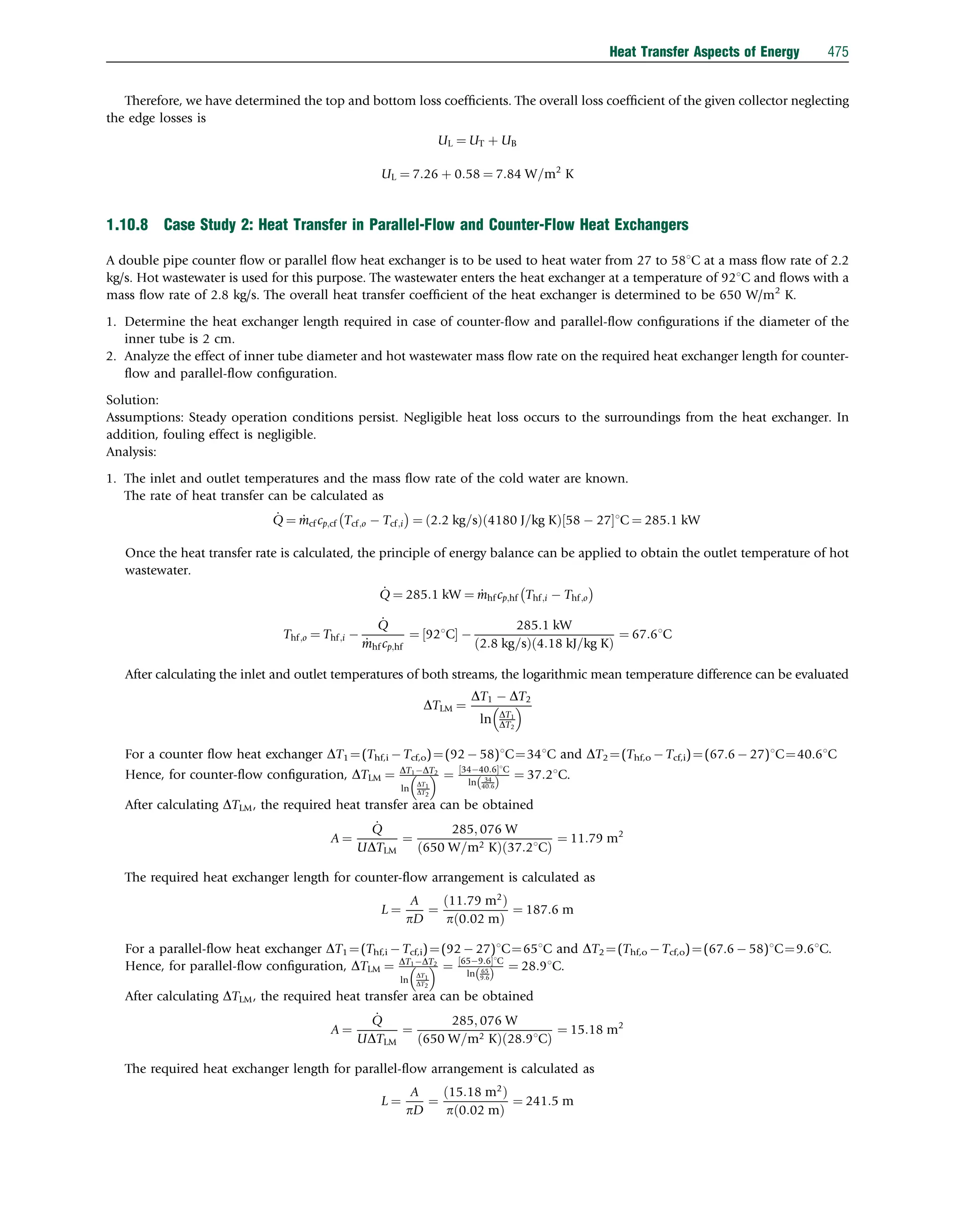
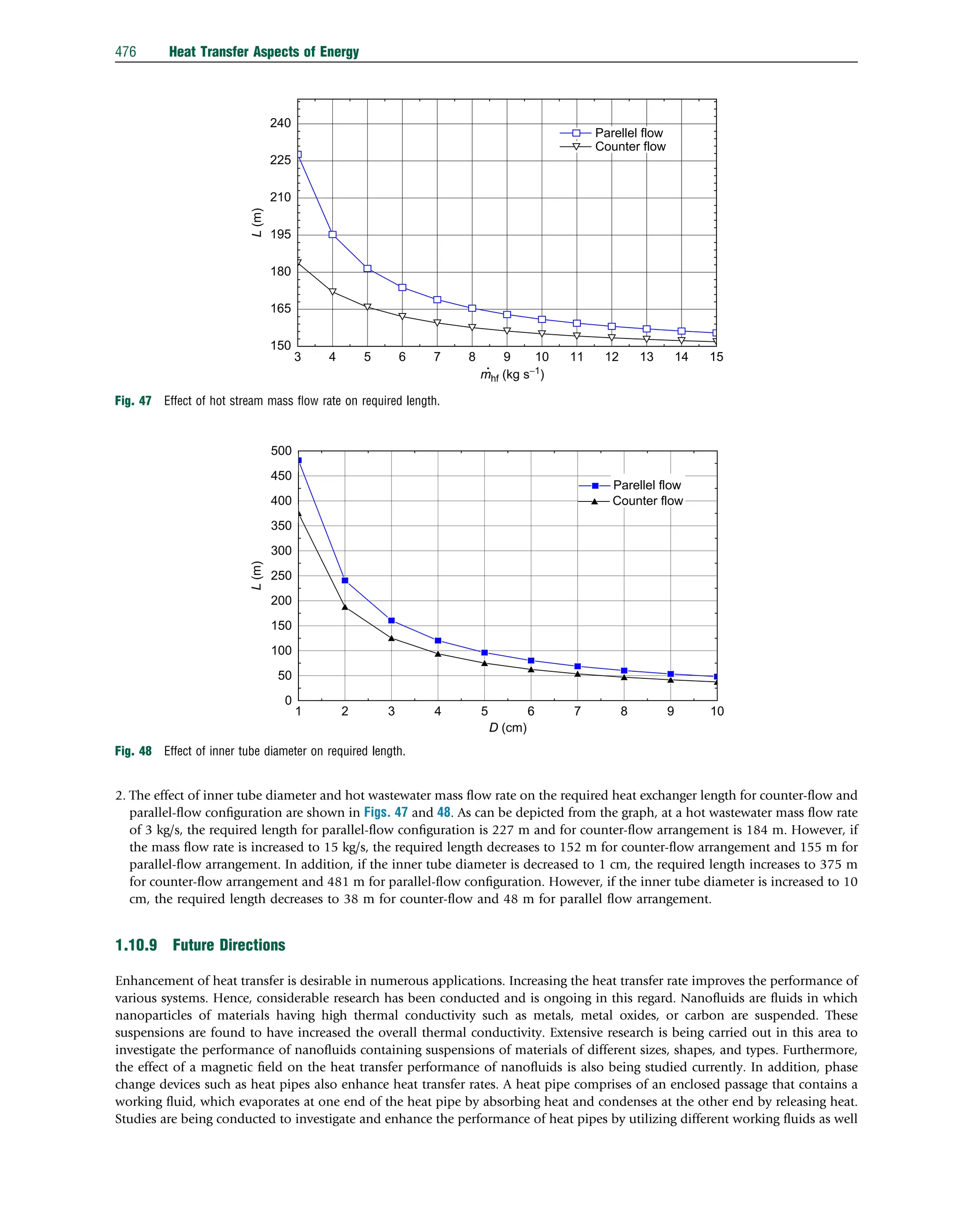
56. as size and shape of heat pipes in different applications. Moreover, composite materials with significantly high thermal con-
ductivity are being investigated for the enhancement of heat transfer in different applications. Various compositions and materials
are being studied in this regard. Extended surfaces such as fins are used extensively in various applications to enhance the heat
transfer rate. Numerous studies are being conducted to investigate the performance of different types, shapes, configurations,
combinations, and materials of fins for different applications. Furthermore, the effect and characteristics of vortex generators with
regard to heat transfer are also being investigated.
1.10.10 Conclusions
This chapter is focused on the heat transfer aspects of energy. The chapter first discusses the first law of thermodynamics and energy
balance, which is the underlying principle for heat transfer analysis. Further, the analysis of different modes of heat transfer for
different types of cases and geometries is discussed. Heat transfer analysis forms an integral part of different aspects of energy
applications. The chapter relates the analysis of heat transfer to different energy applications. For instance, heat transfers though
walls or windows, which are essential to determine the heating or cooling load of a building, are discussed and analyzed.
Furthermore, determining the rate of heat loss from solar collectors, which is essential to analyze their performance, is also
discussed. In addition, analysis of heat exchangers, which is essential in numerous applications, is also briefly described. Analyzing
the rate of heat loss or gain by a given system is vital to study its overall performance.
References
[1] Dincer I. Analytical modelling of heat transfer from a single slab in freezing. Int J Energy Res 1995;19(3):227–33.
[2] Dincer I. Transient temperature distributions in spherical and cylindrical food products subjected to hydrocooling. Int J Energy Res 1994;18(8):741–9.
Further Reading
Cengel YA, Boles MA. Thermodynamics: an engineering approach. Boston: McGraw-Hill; 2002.
Cengel YA, Ghajar AJ. Heat and mass transfer: fundamentals applications. New York, NY: McGraw-Hill Education; 2015.
Dincer I. Thermodynamics, exergy and environmenptal impact. In: Proceedings of the ISTP-11, the eleventh international symposium on transport phenomena, Hsinchu, Taiwan;
1998. p.121–125, 29 November–3 December, 1998.
Duffie JA, Beckman WA. Solar engineering of thermal processes. Hoboken, NY: Wiley; 2013.
Relevant Websites
https://www.asme.org/engineering-topics/heat-transfer
American Society of Mechanical Engineers.
https://www.britannica.com/science/heat-transfer
Encyclopedia Britannica.
https://www.thermalfluidscentral.org/encyclopedia/index.php/Main_Page
Thermal-FluidsPedia.
Heat Transfer Aspects of Energy 477