Download to read offline


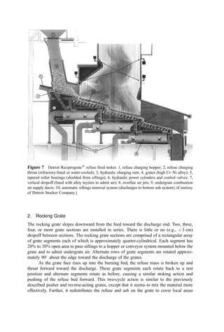
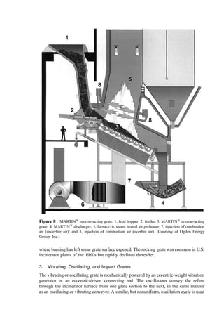
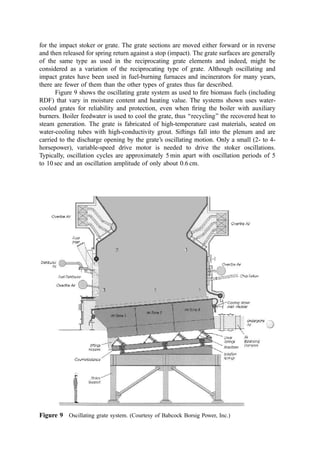
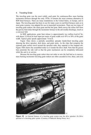
![Preface to the Third Edition
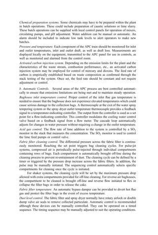
The third edition of Combustion and Incineration Processes incorporates technology
updates and additional detail on combustion and air pollution control, process evaluation,
design, and operations from the 1990s. Also, the scope has been expanded to include: (1)
additional details and graphics regarding the design and operational characteristics of
municipal waste incineration systems and numerous refinements in air pollution control,
(2) the emerging alternatives using refuse gasification technology, (3) lower-temperature
thermal processing applied to soil remediation, and (4) plasma technologies as applied to
hazardous wastes. The accompanying diskette offers additional computer tools.
The 1990s were difficult for incineration-based waste management technologies in
the United States. New plant construction slowed or stopped because of the anxiety of the
public, fanned at times by political rhetoric, about the health effects of air emissions. Issues
included a focus on emissions of ‘‘air toxics’’ (heavy metals and a spectrum of organic
compounds); softening in the selling price of electricity generated in waste-to-energy
plants; reduced pressure on land disposal as recycling programs emerged; and the opening
of several new landfills and some depression in landfilling costs. Also, the decade saw
great attention paid to the potential hazards of incinerator ash materials (few hazards were
demonstrated, however). These factors reduced the competitive pressures that supported
burgeoning incinerator growth of the previous decade.
Chapters 13 and 14 of this book, most importantly, give testimony to the great
concern that has been expressed about air emissions from metal waste combustion
(MWC). This concern has often involved strong adversarial response by individuals in
potential host communities that slowed or ultimately blocked the installation of new
facilities and greatly expanded the required depth of analysis and intensified regulatory
agency scrutiny in the air permitting process. Further, the concern manifested itself in
more and more stringent air emission regulations that drove system designers to
incorporate costly process control features and to install elaborate and expensive trains
of back-end air pollution control equipment. A comparative analysis suggests that MWCs
are subject to more exacting regulations than many other emission sources [506]. This is](https://image.slidesharecdn.com/combustionandincinerationprocesses-220507104234-264c413a/85/COMBUSTION_AND_INCINERATION_PROCESSES-pdf-5-320.jpg)


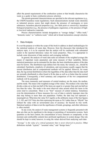
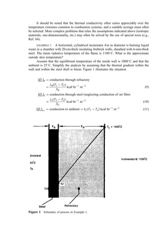
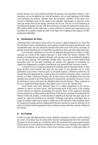
![The approximate heat loss between 1200
and 300
C is 18,140 kcal.
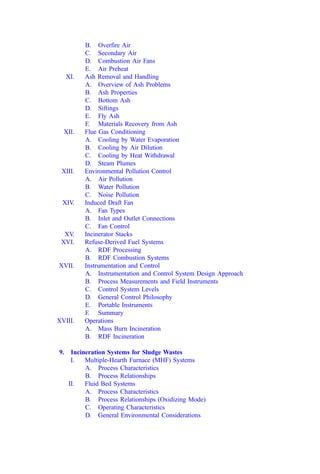
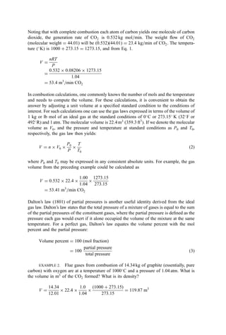
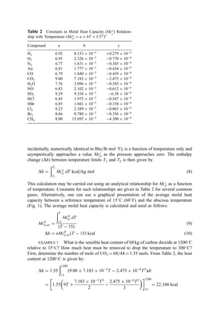
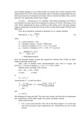
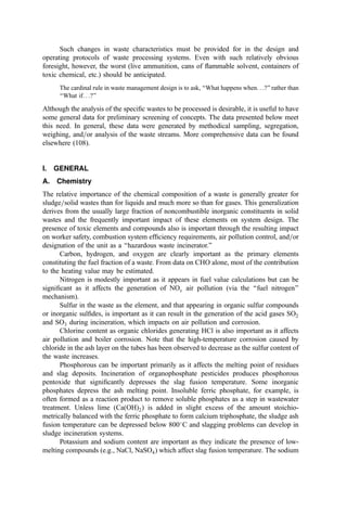
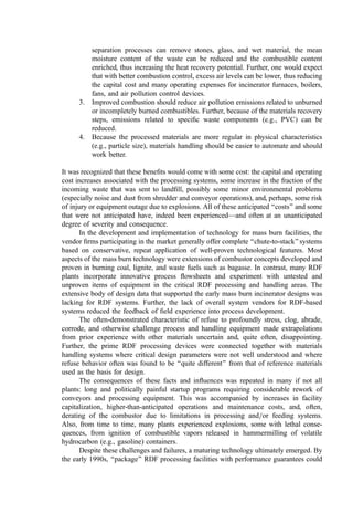
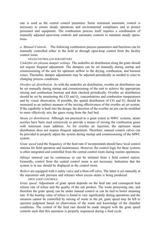
3. Sensible Heat of Solids
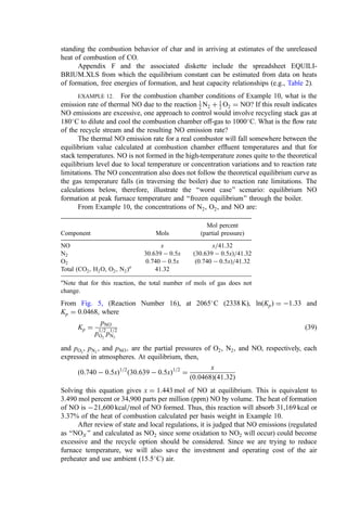
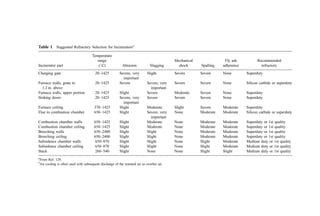
Kopp’s rule [Eq. (11)] (432) can be used to estimate the molar heat capacity (Mcp) of solid
compounds. Kopp’s rule states that
Mcp ¼ 6n kcal=kg mol
C ð11Þ
where n equals the total number of atoms in the molecule.
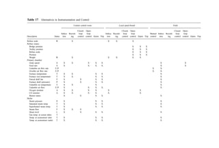
Building on Kopp’s rule, Hurst and Harrison (433) developed an estimation
relationship for the Mcp of pure compounds at 25
C:
Mcp ¼
P
n
i¼1
NiDEi kcal=kg mol
C ð12Þ
where n is the number of different atomic elements in the compound, Ni is the number of
atomic elements i in the compound, and DEi is the value from Table 3 for the ith element.
Voskoboinikov (391) developed a functional relationship between the heat capacity
of slags Cp (in cal=gram
C) and the temperature T ð
C) given as follows.
For temperatures from 20
to 1350
C:
Cp ¼ 0:169 þ 0:201 103
T 0:277 106
T2
þ 0:139 109
T3
þ 0:17 104
Tð1 CaO=SÞ ð12aÞ
where S is the sum of the dry basis mass percentages SiO2 þ Al2O3 þ FeOþ
MgO þ MnO.
For temperatures from 1350
to 1600
C:
Cp ¼ 0:15 102
T 0:478 106
T2
0:876 þ 0:016ð1 CaO=SÞ ð12bÞ
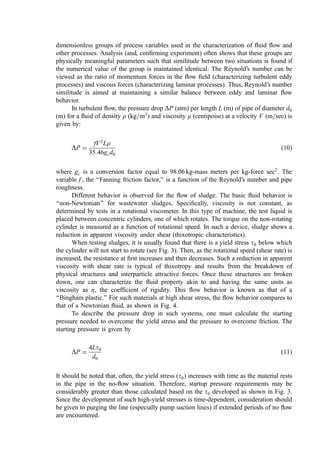
For many inorganic compounds (e.g., ash), a mean heat capacity of 0.2 to 0.3 kcal=kg
C is
a reasonable assumption.
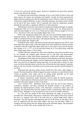
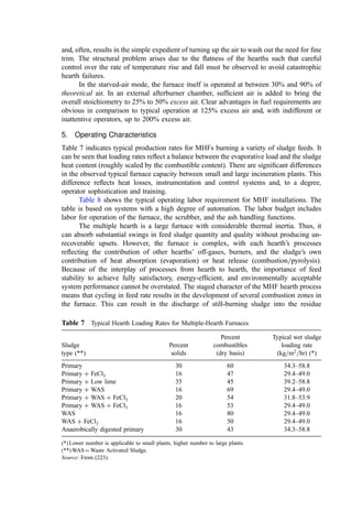
Table 3 Atomic Element Contributions to Hurst and Harrison Relationship
Element DEi Element DEi Element DEi
C 2.602 Ba 7.733 Mo 7.033
H 1.806 Be 2.979 Na 6.257
O 3.206 Ca 6.749 Ni 6.082
N 4.477 Co 6.142 Pb 7.549
S 2.953 Cu 6.431 Si 4.061
F 6.250 Fe 6.947 Sr 6.787
Cl 5.898 Hg 6.658 Ti 6.508
Br 6.059 K 6.876 V 7.014
I 6.042 Li 5.554 W 7.375
Al 4.317 Mg 5.421 Zr 6.407
B 2.413 Mn 6.704 All other 6.362](https://image.slidesharecdn.com/combustionandincinerationprocesses-220507104234-264c413a/85/COMBUSTION_AND_INCINERATION_PROCESSES-pdf-32-320.jpg)


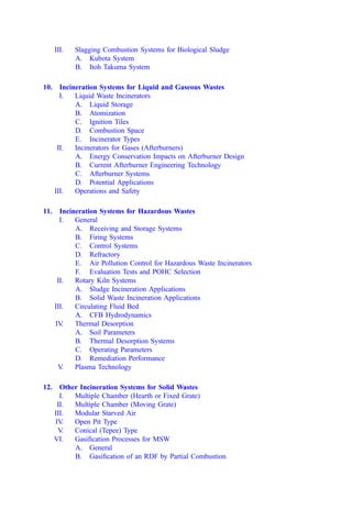
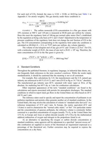
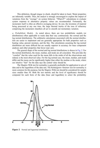
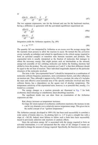
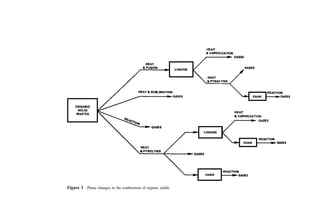
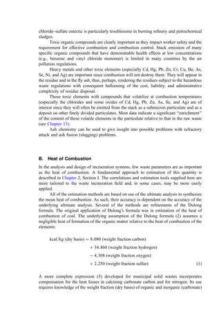
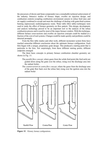
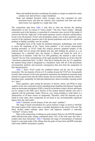
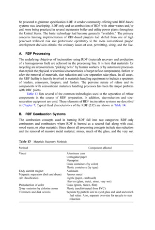
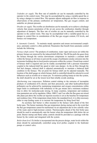
![Radiation loss is the expression used to describe the third major heat loss: leakage of
heat into the surroundings by all modes of heat transfer. Radiation losses increase in
proportion to the exposed area of hot surfaces and may be reduced by the use of insulation.
Since heat loss is area-dependent, the heat loss (expressed as percentage of total heat
release) generally increases as the total heat release rate decreases. The American Boiler
Manufacturers’ Association developed a dimensional algorithm [Eq. (13)] with which to
estimate heat losses from boilers and similar combustors (180). The heat loss estimate is
conservative (high) for large furnaces:
radiation loss ¼
3:6737
C
HR C
FOP
0:6303
ekWtype
ð13Þ
where for the radiation loss calculated in kcal=hr (or Btu=hr):
C ¼ constant: 1.0 for kcal=hr (0.252 for Btu=hr)
HR ¼ design total energy input (fuel þ waste heat of combustion þ air preheat) in
kcal=hr (or Btu=hr)
FOP ¼ operating factor (actual HR as decimal percent of design HR)
k ¼ constant dependent on the method of wall cooling and equal to
Wall cooling method k
Not cooled þ0.0
Air-cooled 0.0013926
Water-cooled 0.0028768
Wtype ¼ decimal fraction of furnace or boiler wall that is air- or water-cooled
II. SYSTEMS ANALYSIS
A. General Approach
1. Basic Data
The basic information used in the analysis of combustion systems can include tabulated
thermochemical data, the results of several varieties of laboratory and field analyses
(concerning fuel, waste, residue, gases in the system), and basic rate data (usually, the flow
rates of feed, flue gases, etc.). Guiding the use of these data are fundamental relationships
that prescribe the combining proportions in molecules (e.g., two atoms of oxygen with one
of carbon in one molecule of carbon dioxide) and those that indicate the course and heat
effect of chemical reactions.
2. Basis of Computation
To be clear and accurate in combustor analysis, it is important to specifically identify the
system being analyzed. This should be the first step in setting down the detailed statement
of the problem. In this chapter, the term basis is used. In the course of prolonged analyses,
it may appear useful to shift bases. Often, however, the advantages are offset by the lack of
a one-to-one relationship between intermediate and final results.
As the first step, therefore, the analyst should choose and write down the reference
basis: a given weight of the feed material (e.g., 100 kg of waste) or an element, or a unit](https://image.slidesharecdn.com/combustionandincinerationprocesses-220507104234-264c413a/85/COMBUSTION_AND_INCINERATION_PROCESSES-pdf-36-320.jpg)


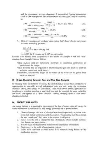
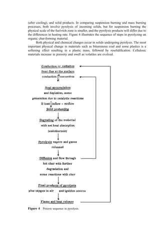
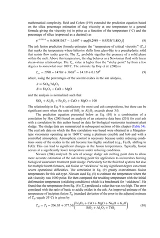
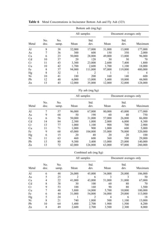
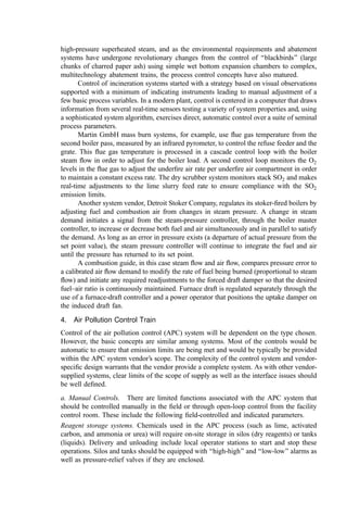
![influence the combustion process or would be important to air pollution or water pollution
assessments. In general, several different samples are used to generate the total analysis
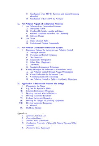
report. Particularly for waste analysis, therefore, some numerical inconsistencies should
not be unexpected.
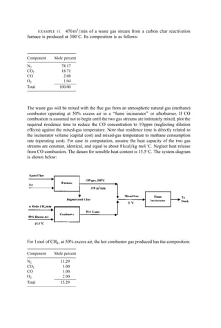
As for the proximate analysis, the testing method can produce uncertain results for
several analysis categories. The weight reported as ‘‘ash’’ will be changed by oxidation of
metals in the sample, by release of carbon dioxide from carbonates, by loss of water from
hydrates or easily decomposed hydroxides, by oxidation of sulfides, and by other reactions.
Also, volatile organic compounds (e.g., solvent) can be lost in the drying step, thus
removing a portion of the fuel chemistry from the sample.
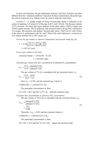
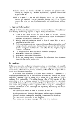
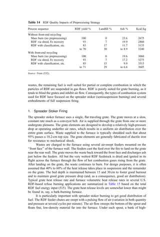
4. Thermochemical Analysis
The heat of combustion of wastes is, clearly, important information in incineration system
analysis. However, one must be cautious in accepting even the mean of a series of
laboratory values (noting that a bomb calorimeter uses only about 1 g of sample) when
there are problems in obtaining a representative sample (see below). For both municipal
and industrial incineration systems, the analyst must also recognize that within the
hardware lifetime waste heat content will almost inevitably change: year to year, season
to season, and, even day to day. This strongly suggests the importance of evaluating the
impact of waste variation on system temperatures, energy recovery, etc. Further, such
likely variability raises legitimate questions regarding the cost-effectiveness of extensive
sampling and analysis programs to develop this type of waste property information.
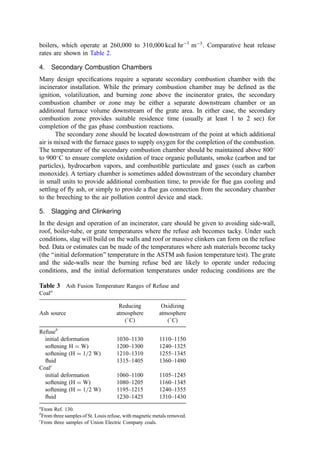
5. Special Analysis
A competent fuels laboratory offers other analysis routines that can provide essential
information for certain types of combustors or process requirements.
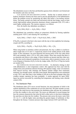
The forms of sulfur analysis breaks down the total sulfur content of the material into
three categories: organic, sulfide (pyritic), and sulfate. The ‘‘organic’’ and ‘‘sulfide’’sulfur
forms will oxidize in an incineration environment, thus contributing to the stoichiometric
oxygen requirement. Oxidation produces SO2 and SO3 (acid gases) that often have
significance in air pollution permits. ‘‘Sulfate’’sulfur is already fully oxidized and, barring
dissociation at very high temperatures, will not contribute to acid gas emissions or
consume alkali in a scrubbing system.
A test for forms of chlorine provides a similar segregation between organically and
inorganically bound chlorine in wastes. Chlorine is a very important element in waste
combustion. Organic chlorine [e.g., in polyvinyl chloride (PVC) and other halogenated
polymers or pesticides] is almost quantitatively converted by combustion processes to
HCl: an acid gas of significance in many state and federal air pollution regulations, an
important contributor to corrosion problems in boilers, scrubbers, and fans, and a
consumer of alkali in scrubbers. Inorganic chlorine (e.g., NaCl) is relatively benign but
contributes to problems with refractory attack, submicron fume generation, etc. Since all
but a few inorganic chlorides are water soluble and few organic chloride compounds show
any significant solubility, leaching and quantification of the soluble chlorine ion in the
leachate provides a simple and useful differentiation between these two types of chlorine
compounds.
An ash analysis is another special analysis. The ash analysis reports the content of
the mineral residue as the oxides of the principal ash cations. A typical ash analysis is
reported as the percent (dry basis) of SiO2, Al2O3, TiO2, Fe2O3, CaO, MgO, P2O5, Na2O,](https://image.slidesharecdn.com/combustionandincinerationprocesses-220507104234-264c413a/85/COMBUSTION_AND_INCINERATION_PROCESSES-pdf-41-320.jpg)


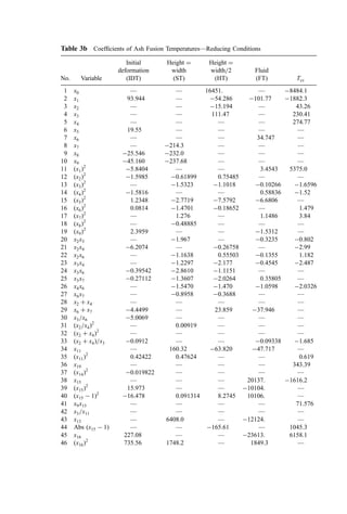
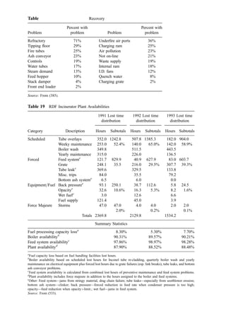
![Table 8 Calculations for Example 8a
Theoretical
Atoms or Combustion moles O2
Line Component kg molesb
product required
1 Carbon (C) 71.0 5.912 CO2 5.912
2 Hydrogen (H2) 9.2 4.563 H2O 2.282
3 Sulfur (S) 3.4 0.106 SO2 0.106
4 Oxygen (O2) 2.1 0.066 — (0.066)
5 Nitrogen (N2) 0.6 0.021 N2 0.0
6 Moisture (H2O) 12.2 0.678 — 0.0
7 Ash 1.5 N=A — 0.0
8 Total 100.0 11.387 8.234
9 Moles nitrogen in stoichiometric airc
(79=21)(8.234)
10 Moles nitrogen in excess air (0.3)(79/21)(8.234)
11 Moles oxygen in excess air (0.3)(8.234)
12 Moles moisture in combustion aird
13 Total moles in flue gas
14 Volume (mole) percent in wet flue gas
15 Orsat (dry) flue gas analysis—moles
16 A. With selective SO2 testing—vol %
17 B. With alkaline CO2 testing only—vol %
18 C. With SO2 loss in testing—vol %
a
Basis: 100 kg of waste.
b
The symbol in the component column shows whether these are kg moles or kg atoms.
c
Throughout this chapter, dry combustion air is assumed to contain 21.0% oxygen by volume and
79.0% nitrogen.
d
Calculated as follows: (0.008=18.016)[Mols N2 in air)(28.016) þ (1 þ % excess air)(Mols O2 for
stoichiometric)(32)] based on the assumption of 0.008 kg water vapor per kg bone-dry air; found
from standard psychrometric charts.
Moles formed in stoichiometric combustion
CO2 H2O SO2 N2 O2 Total
5.912 0.0 0.0 0.0 0.0 5.912
0.0 4.563 0.0 0.0 0.0 4.563
0.0 0.0 0.106 0.0 0.0 0.106
0.0 0.0 0.0 0.0 0.0 0.0
0.0 0.0 0.0 0.021 0.0 0.021
0.0 0.678 0.0 0.0 0.0 0.678
0.0 0.0 0.0 0.0 0.0 0.0
5.912 5.241 0.106 0.021 0 11.280
30.975 30.975
9.293 9.293
2.470 2.470
0.653 0.538
5.912 5.894 0.106 40.289 2.470 54.671
10.81 10.78 0.194 73.69 4.52 100.000
5.912 0.106 40.289 2.47 48.777
12.12 N=A 0.22 82.60 5.06 100.0
12.34 N=A N=A 82.60 5.06 100.0
12.15 N=A N=A 82.78 5.08 100.0](https://image.slidesharecdn.com/combustionandincinerationprocesses-220507104234-264c413a/85/COMBUSTION_AND_INCINERATION_PROCESSES-pdf-48-320.jpg)


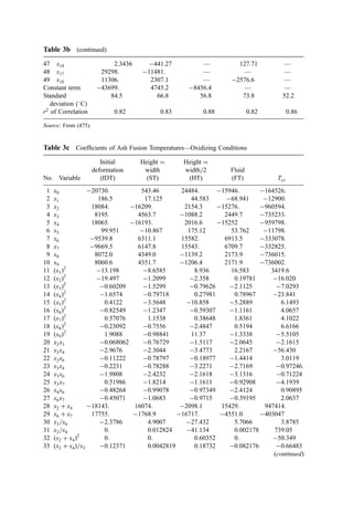
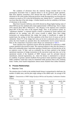
![Table 10 Computation of Heat Content of Flue Gases from Combustion of Benzene Waste at 10% Excess Air
A Assumed temperature ð
CÞ 180.0 500.0 1000.0 1500.0 2000.0 2600.0
B A15.5 ð
CÞ 164.5 484.5 984.5 1484.5 1984.5 2484.5
C Mcp-av for N2 at A
Ca
6.93 7.16 7.48 7.74 7.95 8.10
D Mcp-av for O2 at A
C 7.17 7.48 7.87 8.13 8.26 8.26
E Mcp-av for H2O at A
C 8.06 8.53 9.22 9.85 10.42 10.93
F Mcp-av for CO2 at A
C 9.67 10.64 11.81 12.57 12.91 12.85
G Mcp-av for Ash at A a
Cb
0.20 0.20 0.20 0.20 0.20 0.20
H Heat content of N2 30.639 (B)(C) 34,905 106,299 225,670 352,249 483,394 616,461
I Heat content of O2 0.740(B)(D) 873 2,685 5,737 8,935 12,136 15,137
J Heat content of H2O 3.880(B)(E) 5,143 16,032 35,203 58,711 80,224 105,410
K Heat content of CO2 6.060(B)(F) 9,643 31,235 70,454 113,055 155,290 193,408
L Heat content of ash 9.3[(B)(G) þ 85]c
306 901 2,622 3,552 4,482 5,412
M Latent heat in water vapor 3.383(10,595)d
35,843 35,843 35,843 35,843 35,843 35,843
N Total heat content of gas ðH þ I þ J þ K þ L þ MÞe
86,713 192,996 375,513 570,330 771,353 971,715
O Kcal=kg-mol of gas 2,099 4,671 9,088 13,803 18,668 23,517
a
Source: Figure 1, kcal=kg mol
C.
b
Specific heat of the ash (kcal=kg
C) for solid or liquid.
c
The latent heat of fusion for the ash (85 kcal=kg) is added at temperatures greater than 800
C, the assumed ash fusion temperature.
d
Latent heat of vaporization at 15:5
C of free water in waste and from combustion of hydrogen in the waste (kcal=kg mol).](https://image.slidesharecdn.com/combustionandincinerationprocesses-220507104234-264c413a/85/COMBUSTION_AND_INCINERATION_PROCESSES-pdf-58-320.jpg)


![Then from the overall reaction at 25
C, the standard free-energy change and, thus, the
Kp298 is given by
DF
298 ¼ 94;260 þ 0 ð54;635 32;808Þ ¼ 6817
ln Kp298 ¼ ð6810Þ=ð298RÞ ¼ 11:50 and Kp298 ¼ 9:90 104
and, from the change in the standard enthalpies of formation,
DH
298 ¼ 94;052 þ 0 ð57;798 26;416Þ ¼ 9838
From the heat capacity constants in Table 2, the DCp function is
DCp ¼ CpCO2
þ CpH2
CpCO CpH2O
¼ 1:37 þ 2:4 103
T 1:394 106
T2
From Eq. (35b),
DH
¼ DH
0 þ 1:37T þ 1:2 103
T2
4:647 107
T3
Substituting DH
¼ 9838 at T ¼ 298
C and solving for DH
0 , DH
0 ¼ 10;321:2. Then,
the temperature relationship for the equilibrium constant [Eq. (36)] is
ln Kp ¼
10;321:2
RT
þ
1:37
R
ln T þ
1:4 103
R
T
4:647 107
2R
T2
þ I
Using the value of ln Kp298 from above, the integration constant I can be evaluated as
I ¼ 9:9817
from which the final expression for ln Kp is
ln Kp ¼ 9:9817 þ
5223
T
þ 0:692 ln T þ 7:07 104
T 1:173 107
T2
For the required Kp at 1000
C (1273.15 K), ln Kp is 0:5877 and Kp ¼ 0:556.
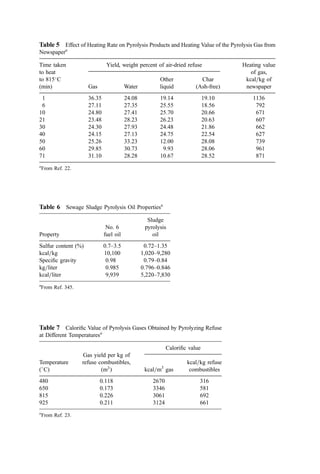
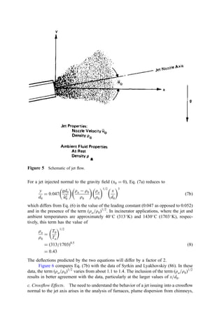
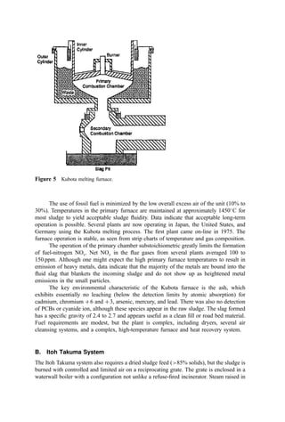
Figure 5 shows the temperature dependence of several reactions of interest in
combustion analysis. Kp is based on partial pressures in atmospheres. Water is as the vapor.
Carbon (solid) is beta-graphite. For combustion calculations, several reactions merit
consideration in evaluating heat and material flows, especially the gas phase reactions
of H2, H2O, CO, CO2, O2, with H2O, CO2, and O2. Note that for reactions involving
solids, the activity of the solid compounds is assumed to be unity. Thus, the ‘‘concentra-
tion’’ or ‘‘partial pressure’’ of carbon or other solids does not enter into the mathematical
formulation.
The partial pressure of the gases in a mixture at atmospheric pressure can be
conveniently equated with the mol fraction (mols of component divided by the total
number of mols in the mixture). This equivalence (Dalton’s law) and its use in the
equilibrium constant formulation is strictly true only for ideal gases. Fortunately, at the
temperatures and pressures typical of most combustion calculations, this is a valid
assumption.
The importance of the reactions described in Fig. 5 relates to both combustion
energetics and pollution control. For example, equilibrium considerations under conditions
near to stoichiometric may show that substantial nitric oxide and carbon monoxide may be
generated. Also, the interactions of H2O, CO, CO2, C, and O2 are important in under-](https://image.slidesharecdn.com/combustionandincinerationprocesses-220507104234-264c413a/85/COMBUSTION_AND_INCINERATION_PROCESSES-pdf-64-320.jpg)


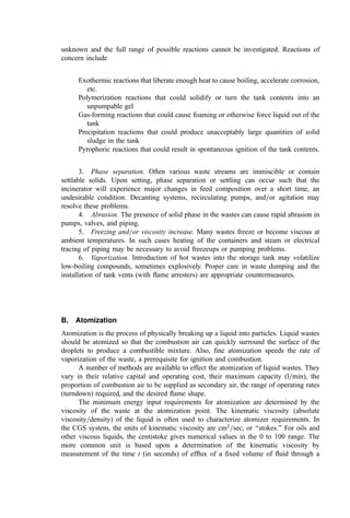
![suggest problems with significant adverse impacts, the real health risk consequence is
often modest to (practically) none. This is due to the low concentration of individual PICs
in the flue gases and, thus, the very low ambient concentrations experienced by even the
‘‘most exposed individual.
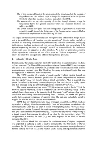
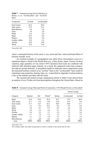
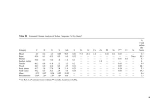
3. Ignition Temperature Data
Based on both kinetic data and data from dilute fume afterburner performance, the ignition
temperature can be determined. Ignition temperature data for both direct flame and
catalytic afterburners are shown in Table 13.
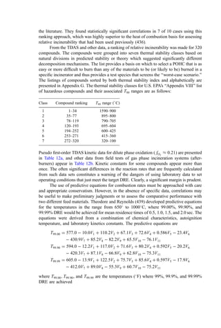
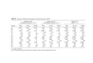
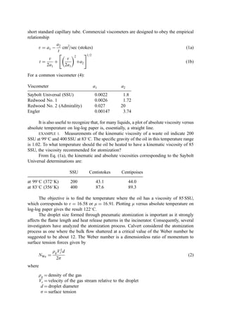
4. Flash Point Estimation
The flash point is the lowest temperature at which a liquid gives off sufficient vapor to
form an ignitable mixture with air near the surface of the liquid. Several standard methods
are available using a closed cup (the preferred method) or an open cup. Flash point is
suggested as a measure of ‘‘ignitability’’ by the U.S. EPA and by regulatory agencies
elsewhere. The EPA defines a liquid as hazardous as a consequence of ignitability if the
closed-cup flash point is less than 60
C. To be protective, the lowest flash point
temperature is usually taken.
Several flash point values are shown in Table 14. Flash points can be estimated using
the method of Shebeko (441) according to the following methodology:
Step 1. From Eqs. 67a and 67b, calculate the vapor pressure of the substance at the
flash point (Psat-fp) as related to the total system pressure P and the numbers of
atoms of carbon (NC), sulfur (NS), hydrogen (NH), halogen (NX), and oxygen
(NO) in the molecule.
Table 13 Ignitition Temperatures of Selected
Compounds [195]
Ignition temperature
(
C)
Compound Thermal Catalytic
Benzene 580 302
Toluene 552 302
Xylene 496 302
Ethanol 392 302
Methyl isobutyl ketone 459 349
Methyl ethyl ketone 516 349
Methane 632 500
Carbon monoxide 609 260
Hydrogen 574 121
Propane 481 260](https://image.slidesharecdn.com/combustionandincinerationprocesses-220507104234-264c413a/85/COMBUSTION_AND_INCINERATION_PROCESSES-pdf-87-320.jpg)
![Step 2. From data or correlations of vapor pressure and temperature, find the
temperature corresponding to the calculated vapor pressure
psat-fp ¼
P
1 þ 4:76ð2b 1Þ
ð67aÞ
b ¼ NC þ NS þ
ðNH NXÞ
4
NO
2
ð67bÞ
EXAMPLE 16. Using the method of Shebeko, estimate the flash point of methyl ethyl
ketone (MEK). Compare the estimated value to the literature value of 1:1
C.
MEK has the atomic formula CH3C2H5CO and, from Eq. 67b, b ¼ 5:5 and
Psat-fp ¼ 15.6 mm Hg at a total pressure of 1 atm. From vapor pressure correlations
available from the literature (e.g., (442)], the vapor pressure of MEK (Pvap) may be
approximated by
Pvap ¼ exp 72:698
6143:6
T
7:5779 lnðTÞ þ 5:6476 106
T2
By successive approximation, T ¼ 8
C.
Table 14 Values of the Flash Point ð
CÞ for Several Substances
Tflash Tflash Tflash Tflash
Compound ð
FÞ ð
CÞ Compound ð
FÞ ð
CÞ
Acetic acid 104.0 40.0 Diethyl ether 20.0 28.9
Acetone 0.0 17.8 Ethyl acetate 24.0 4.4
Benzene 12.0 11.1 Ethylene glycol 232.0 111.1
Butyl acetate 216.0 102.2 Furfural 140.0 60.0
Chlorobenzene 90.0 32.2 Methyl alcohol 54.0 12.2
Cottonseed oil 590.0 310.0 Methyl ethyl ketone 30.0 1.1
o-Cresol 178.0 81.1 Naphthalene 174.0 78.9
Cyclohexanol 154.0 67.8 Phenol 175.0 79.4
Decane 115.0 46.1 Toluene 40.0 4.4](https://image.slidesharecdn.com/combustionandincinerationprocesses-220507104234-264c413a/85/COMBUSTION_AND_INCINERATION_PROCESSES-pdf-88-320.jpg)


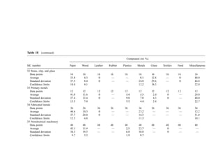
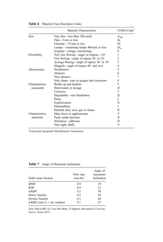
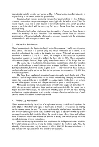
![Table 10a Solid Waste Weight Percent Characterization Data (1988, 1990) [291]
Waste category
Indian-
apolis, IN
Kauai,
HI
King
Co., WA
Bergen
Co., NJ
Monroe
Co., NY
Paper 38 26 27 44 42
Plastics 8 7 7 9 10
Yard debris 13 20 19 9 7
Miscellaneous organics 22 24 31 17 24
Glass 7 5 4 7 10
Aluminum 1 1 1 1 1
Ferrous metal 4 6 3 5 5
Nonferrous metal 0 1 1 4 0
Miscellaneous inorganics 0 3 7 5 0
Other 0 9 0 3 0
Waste category
Ann
Arbor,
MI
Portland,
OR
San
Diego,
CA
Santa
Cruz
Co., CA
National
estimate
Paper 29 29 26 33 34
Plastics 8 7 7 8 9
Yard debris 8 11 21 15 20
Miscellaneous organics 39 33 23 18 20
Glass 4 3 4 7 7
Aluminum 1 1 1 1 1
Ferrous metal 5 7 3 5 7
Nonferrous metal 2 0 0 0 0
Miscellaneous inorganics 2 9 6 6 2
Other 2 1 10 7 0
Table 10b Standard Deviations of Solid Waste Characterization Data (Percent of Reported
Average Weight Percent Values) [291]
Waste
category
Portland,
OR
Cincinatti,
OH
Bergen Co.,
NJ
Rochester,
NY
Sacremento,
CA
Paper 6 20 19 13 14
Plastics 14 10 35 19 3
Yard debris 11 26 28 26 17
Misc. organics 12 52 86 32 17
Glass 24 16 32 46 2
Aluminum 35 48 50 76 56
Ferrous metal 13 27 54 29 15
Nonferrous metal 63 137 48 161 80
Misc. inorganics 11 54 59 — 30](https://image.slidesharecdn.com/combustionandincinerationprocesses-220507104234-264c413a/85/COMBUSTION_AND_INCINERATION_PROCESSES-pdf-134-320.jpg)


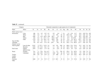
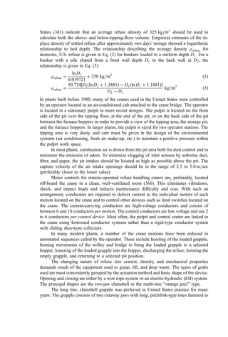
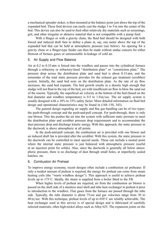
![establish average chemical composition, heat content, and the like requires assumptions of
questionable accuracy, it is a necessary compromise. Typically, several (perhaps one to
three) tons of waste from a 200 to 1000 ton=day waste flow are analyzed to produce a
categorical composition. Then a still smaller sample is hammermilled and mixed, and a
500-mg sample is taken. Clearly, a calorific value determination on the latter sample is, at
best, a rough reflection of the energy content of the original waste.
1. Chemical Analysis
Stepping from the categorical analysis to a mean chemical analysis provides the basis for
stoichiometric calculations. The macrochemistry of waste (the percentage of the major
chemical constituents carbon, hydrogen, oxygen, sulfur, nitrogen, chlorine, and ash) is an
important input to estimates of heat content, combustion air requirements, incinerator mass
balances, etc. The microchemistry of waste (the content of heavy metals and other
environmentally important species present at the parts per million level) is also important
in revealing potential air or ash emission problems.
a. Mixed Municipal Refuse
MAJOR Chemical Constituents. Chemical data for average municipal refuse compo-
nents based on the mixed refuse of Table 8 are presented in Tables 20 and 21. Although
these data may not be at all representative of the material of interest in a given design
effort, the general approach to data analysis presented here may be used. The process
begins with refuse categorical compositions (such as Table 6) and incorporates the effects
of the moisture exchange processes discussed above to produce the baseline refuse
elemental statistics used in heat and material balance computations, etc.
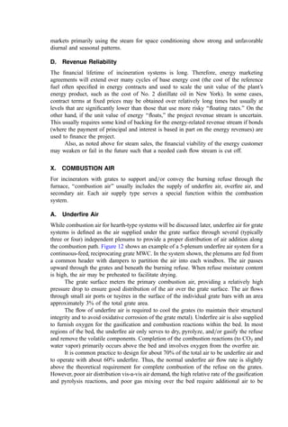
MINOR Chemical Constituents. Increasing interest in the emission rate of metals
with health effects (an important part of the class of air pollutants called ‘‘air toxics) leads
to a need to understand the sources and typical concentrations of many of the trace
elements in waste streams. These concentrations, clearly, vary widely in different waste
components and even within relatively narrow categories of waste. Thus, data on ‘‘typical’’
concentrations must be used with appropriate caution. Table 22 indicates the result of three
extensive analyses of the trace metal concentrations in mixed municipal refuse (455, 456,
457).
A detailed breakdown of several of the important trace elements was made for
wastes delivered to the Burnaby, British Columbia (serving greater Vancouver) MWC
(454). The analytical results for a wide range of individual waste components are shown in
Table 23.
b. Specific Waste Components. Data for specific waste components are given in Table 24.
These data may be used when detailed categorical analyses are available or when one
wishes to explore the impact of refuse composition changes.
It is of importance to distinguish between the two types (soluble and insoluble) of
chlorine compounds found in refuse. The most important soluble chlorine compounds are
sodium and calcium chloride. These compounds (substantially) remain as solid inorganic
salts in the bottom ash and fly ash. The insoluble chlorine compounds are principally
chlorine-containing organic compounds [e.g., polyvinyl chloride (PVC), polyvinylidene
chloride (Saran), etc.] that form HCl in combustion processes and thus generate a
requirement for acid gas control. Data on the distribution of the two forms of chlorine
(378) are shown in Table 25.
(text continues on p. 140)](https://image.slidesharecdn.com/combustionandincinerationprocesses-220507104234-264c413a/85/COMBUSTION_AND_INCINERATION_PROCESSES-pdf-144-320.jpg)


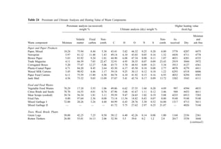
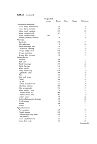
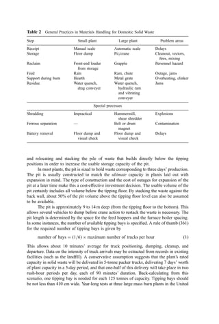
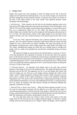
![2. Bulk Density
In many smaller municipalities, weighing scales for refuse vehicles are not available. In
such circumstances, data is often gathered on a volumetric basis. Bulk density data are
presented in Table 26.
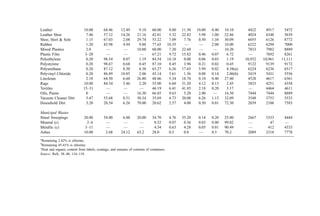
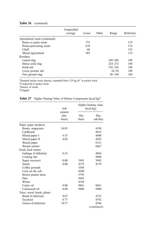
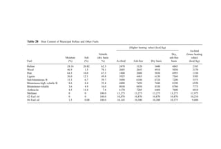
3. Thermal Parameters
Once a weight-basis generation rate is established, data on the heating value of waste
components are of great interest to the combustion engineer. The information in Table 27
is presented to supplement the data in Table 24.
4. Municipal Refuse as a Fuel
Electric power plants and industrial combustion systems represent a rich source of data and
proven design experience for understanding and improving incineration systems. To use
these data, however, it is necessary to appreciate the similarities and differences between
municipal refuse and its associated combustion parameters and those for other fuels.
a. Heat Content. Municipal refuse, though quite different from high-rank coals and oil,
has considerable similarity to wood, peat, and lignite (Table 28). It would be reasonable,
therefore, to seek incinerator design concepts in the technology developed for the
combustion of the latter materials. Refuse does, however, have distinguishing character-
istics, such as its high total ash content, which may require more extensive ash-handling
Table 25 Soluble and Insoluble Chlorine Content of Refuse Constituents [378] (Mass Percent—
Dry Basis)
A. Baltimore County, MD
Waste Total Std. Soluble Std. Insoluble Std.
category % Cl2 dev. % Cl2 dev. % Cl2 dev.
Paper 0.251 0.0063 0.088 0.0077 0.163 0.0099
Plastics, soft 0.055 0.0100 0.004 0.0013 0.051 0.0101
Plastics, hard 0.083 0.0326 0.000 0.0000 0.083 0.0326
Wood=vegetable 0.005 0.0018 0.003 0.0007 0.002 0.0009
Textiles 0.019 0.0090 0.006 0.0031 0.013 0.0095
‘‘Fines’’ 0.042 0.0053 0.009 0.0011 0.033 0.0054
Total 0.455 0.0363 0.110 0.0085 0.344 0.0373
B. Brooklyn, NY
Waste Total Std. Soluble Std. Insoluble Std.
category % Cl2 dev. % Cl2 dev. % Cl2 dev.
Paper, unbleached 0.211 0.0702 0.140 0.0618 0.071 0.0935
Paper, bleached 0.013 0.0015 0.007 0.0017 0.007 0.0023
Plastics, soft 0.123 0.0427 0.007 0.0014 0.117 0.0427
Plastics, hard 0.332 0.1038 0.009 0.0049 0.323 0.1039
Wood=vegetable 0.056 0.0145 0.023 0.0026 0.034 0.0147
Textiles 0.020 0.0102 0.007 0.0028 0.013 0.0106
‘‘Fines’’ 0.131 0.1141 0.022 0.0114 0.109 0.1147
Total 0.886 0.1757 0.215 0.0632 0.674 0.1869
(text continues on 146)](https://image.slidesharecdn.com/combustionandincinerationprocesses-220507104234-264c413a/85/COMBUSTION_AND_INCINERATION_PROCESSES-pdf-155-320.jpg)


![significantly different than the combustible content due to a high calcium and=or ferric
hydroxide content.
The heat of combustion of wastewater sludges can be estimated from the ultimate
chemical analysis of the sludge using the Dulong, Chang, or Boie relationships [Eqs. (3),
(4), and (5)]. However, comparison (204) of predictions using these relationships with data
from fuels laboratories for a set of over 80 sludge samples from a variety of wastewater
plants showed that these equations always predict high by an average of about 9%, 17%,
and 12%, respectively. A modification of the Dulong equation for application to sludge
that, on average, predicts low by only about 6% develops the moisture, ash-free heat of
combustion by
kcal=kg ¼ 5;547C þ 18;287H2 1;720O2 þ 1;000N2 þ 1;667S þ 627Cl
þ 4;333P ð12Þ
where C, H, S, etc. are the decimal percents of carbon, hydrogen, sulfur, etc., evaluated on
a dry, ash-free basis.
The heat of combustion can be expected to vary over time. Data indicate that
digested sludges fall into the low end of the heat of combustion range and heat-treated
(e.g., wet oxidation) sludges fall into the high range.
b. Energy Parameter. In comparison to many other combustion systems, the sludge
incinerator must cope with a fuel having an exceptionally high ash and moisture content.
Thus, the balance between the fuel energy in the combustible, the burdensome latent heat
demand of the moisture, and the dilution effect of the ash is especially important and
powerful. Consequently, numerous thermal studies are inevitably conducted where the
percent solids is carried as the independent parameter and dependent parameters such as
fuel use, steam generated, etc., are derived. It is both inconvenient and aggravating that the
use of ‘‘percent solids’’ as a correlating variable (1) produces nonlinear plots and (2) does
not represent a sludge property that truly is a measure of quality. That is, it is not always
beneficial to increase percent solids (as, say, through adding an inorganic sludge condition
aid). A more useful variable for such investigations is the ‘‘energy parameter’’ (EP), which
combines in a single term the heat and material balance for the combustion of sludge or
other fuels or wastes. The EP is calculated as follows:
EP ¼
ð1 SÞ 106
SBV
kg H2O per million kcal ð13Þ
where
S ¼ decimal percent solids
V ¼ decimal percent volatile
B ¼ heat of combustion ðkcal=kg volatileÞ
The advantage in using the EP instead of percent solids to correlate thermochemical
calculations is that EP correlations are usually linear, whereas, over broad ranges, the
percent solids correlations are strongly curved. It can be noted that for a given percent
excess air the EP collapses the heat effects of water evaporation, flue gas heating, and
waste-derived energy supply into a single term. Using the energy parameter, for example,
fuel requirement and steam-raising potential for sludge incineration correlate linearly.
Further, a reduction in EP is always a benefit: Less fuel is always needed or more energy
recovered.](https://image.slidesharecdn.com/combustionandincinerationprocesses-220507104234-264c413a/85/COMBUSTION_AND_INCINERATION_PROCESSES-pdf-172-320.jpg)
![be mixed with water before using), which can be rammed into place to form
monolithic structures.
Castable and gunning mixes, which are poured or sprayed (gunned), respectively, to
form large monolithic structures.
Mortar and high-temperature cements.
Granular materials such as dead-burned dolomite, dead-burned magnesite and
ground quartzite.
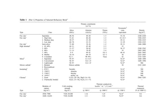
1. Composition of Refractories
Table 1 indicates the primary constituents of many refractories commonly used in
incineration applications. It can be seen that most fireclay alumina and silica refractory
materials are composed of mixtures of alumina (Al2O3) and silica (SiO2) with minor
constituents, including titania (TiO2), magnesite (MgO), lime (CaO), and other oxides. In
high-abrasion areas or where resistance to thermal shock and=or high-thermal conductivity
is important, silicon carbide is also incorporated.
The minerals that constitute refractory materials exhibit properties of acids or bases
as characterized by electron donor or receptor behavior. Acidic oxides include silica,
alumina, and titania, and basic oxides include those of iron, calcium, magnesium, sodium,
potassium, and chromium. The fusion temperatures and compatibility of refractory pairs or
slags and refractory is related especially to the equivalence ratio of the basic to acidic
constituents.
The mineral deposits from which the fire clays are obtained include (1) the hydrated
aluminum silicates (e.g., kaolinite) and flint clays, which contribute strength, refractori-
ness, and dimensional stability, and (2) the plastic and semiplastic ‘‘soft clays,’’ which
contribute handling strength. Bauxite or diaspore clays, precalcined to avoid high
shrinkage in the firing of refractory products, are the principal source of alumina for
high-alumina refractory (greater than 45% alumina).
Basic refractories incorporate mixtures of magnesite (usually derived from magne-
sium hydroxide precipitated from sea water, bitterns, or inland brines), chrome ore, olivine
[a mineral incorporating mixed magnesium, silicon, and iron oxides with forsterite
(2MgOSiO2) predominating], and dolomite, a double carbonate of calcium and magne-
sium.
2. Properties of Refractories
a. Refractory Structure. At room temperature, refractory products consist of crystalline
material particles bonded by glass and=or smaller crystalline mineral particles. As the
temperature increases, liquid phase regions develop. The mechanical properties of the
refractory at a given temperature depend on the proportion and composition of the solid
minerals, glassy structure, and fluid regions.
In the manufacture of refractory products, unfired or ‘‘green’’ refractory masses are
often heated or ‘‘fired’’ in a temperature-controlled kiln to develop a ceramic bond between
the larger particles and the more or less noncrystalline or vitrified ‘‘groundmass.’’ In firing,
a high degree of permanent mechanical strength is developed. For any given refractory
composition, however, there exists an upper temperature limit above which rapid and
sometimes permanent changes in strength, density, porosity, etc., can be expected. This
upper limit is often a critical parameter in the selection of refractory for a given service.
The evaluation of the high-temperature softening behavior of fireclay and some high-
alumina refractory materials is often accomplished by determination of the pyrometric](https://image.slidesharecdn.com/combustionandincinerationprocesses-220507104234-264c413a/85/COMBUSTION_AND_INCINERATION_PROCESSES-pdf-175-320.jpg)


![and lignitic when
Fe2O3 CaO þ MgO
A slagging index (Rs) giving an indication as to the probable severity of slagging can be
formed from the ratio of basic oxides to acidic oxides and the sulfur content (for
bituminous ash). Using the definition based on weight percent of oxides:
B ¼ CaO þ MgO þ Fe2O3 þ Na2O þ K2O ð21aÞ
A ¼ SiO2 þ Al2O3 þ TiO2 ð21bÞ
S ¼ weight percent sulfur on a dry basis
Rs ¼ BS=A ð22Þ
and the slagging potential is given as follows:
Rs 0:6 low 2:0 Rs 2:6 high
0:6 Rs 2:0 medium 2:6 Rs severe
For lignitic ash, the slagging index Rs
* is based on the ash fusibility temperatures given IT
as the initial deformation temperature and HT as the hemispherical temperature:
Rs
* ¼
ðmaximum HTÞ þ 4ðminimum ITÞ
5
ð23Þ
Babcock and Wilcox (532) have found that the most accurate method to predict slagging
potential is based on a viscosity index Rvs based on measurements of the temperature (
F)
where the slag viscosity is 250 poise in an oxidizing atmosphere and 10,000 poise in a
reducing atmosphere (T250-oxid and T10;000-reduc, respectively). The viscosity index is given
by
Rvs ¼
ðT250-oxidÞ ðT10;000-reducÞ
54:17fs
ð24Þ
where fs is a correlation factor given by
fs ¼ 0:5595 1016
T5:3842
ð25Þ
and the slagging potential is given as follows:
Rvs 0:5 low 1:0 Rvs 2:0 high
0:5 Rvs 1:0 medium 2:0 Rvs severe
For bituminous ash, the fouling index Rf is based on the basic and acidic oxide ratios [Eqs.
(21a) and (21b)] and the percentage of sodium oxide in the ash:
Rf ¼
B
A
xNa2O ð26Þ
and the fouling potential is given as follows:
Rf 0:2 low 0:5 Rf 1:0 high
0:2 Rf 0:5 medium 1:0 Rf severe](https://image.slidesharecdn.com/combustionandincinerationprocesses-220507104234-264c413a/85/COMBUSTION_AND_INCINERATION_PROCESSES-pdf-209-320.jpg)


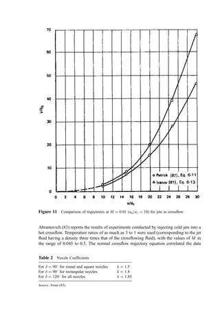
![Figure 2 Relation between coal characteristics and size of combustion space required in USBM test furnace at combustion rate of 50 lb hr1
ft2
and 50%
excess air. Numbers on graphs are the percentage of the heat of combustion of the original coal which appears as unreleased heat of combustion in the furnace
gases. [From (68).]](https://image.slidesharecdn.com/combustionandincinerationprocesses-220507104234-264c413a/85/COMBUSTION_AND_INCINERATION_PROCESSES-pdf-217-320.jpg)
![improved, yet some fraction of the combustible still enters the boiler passes. Figure 3(c)
shows the effect of further increases in the overfire air plenum pressure. Under these latter
conditions, combustion is complete within the furnace volume. For these tests, Mayer
employed jets directed toward the bed just beyond the ignition arch.
Also in the 1930s, developments in fluid mechanics by Prandtl and others provided
mathematical and experimental correlation on the behavior of jets. Application of this
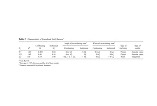
Table 1 Chemical Characteristics of Coal and Refusea
Pocahontas Pittsburgh Illinois
Item Characteristicsb
coal coal coal Refuse
1 Volatile matter 18.05 34.77 46.52 88.02
2 Fixed carbon 81.95 65.23 53.48 11.99
3 Total carbon 90.50 85.7 79.7 50.22
4 Volatile carbon (item 3 minus item 2) 8.55 20.47 26.22 38.22
5 Available hydrogen 3.96 4.70 3.96 1.57
6 Ratio volatile C to available H2 2.16 4.35 6.60 24.34
7 Oxygen 3.32 5.59 10.93 41.60
8 Nitrogen 1.19 1.73 1.70 1.27
9 Percentage of moisture accompa-
nying 100% of MAF coal or
refuse
2.53 2.88 22.07 55.19
10 Product of items 1 and 6 39 151 307 2142
11 Ratio of oxygen to total carbon 0.0367 0.0652 0.137 0.828
12 Total moisture in furnace per
kilogram of coal or refuse
reduced to MAF basis
(kilogram)
0.409 0.501 0.700 1.161
a
Data on coal are from Ref. 68; data on refuse are from Ref. 21.
b
Items 1 through 8 and 11: percent on moisture and ash-free basis (MAF).
Figure 3 Lines of equal heating value (kcal per standard cubic meter) of flue gas firing low-
volatile bituminous coal at a rate of 137 kg m2
hr1
: (a) No overfire air, (b) overfire air pressure
13 mm Hg (7 in. H2O), (c) overfire air pressure 18.7 mm Hg (10 in. H2O). [From (72).]](https://image.slidesharecdn.com/combustionandincinerationprocesses-220507104234-264c413a/85/COMBUSTION_AND_INCINERATION_PROCESSES-pdf-218-320.jpg)
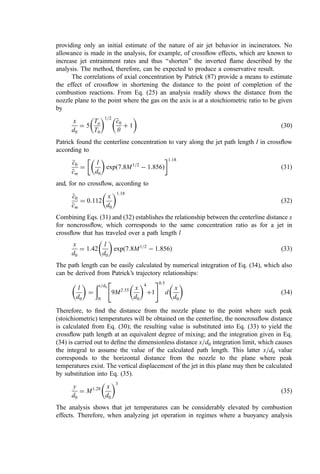
![understanding to furnace situations was presented in some detail by Davis (73). His
correlations, although based on greatly simplified assumptions, were of considerable
interest to furnace designers at that time. As an example of the applicability of his work,
Davis explored the trajectories anticipated for jets discharging over coal fires and
compared his calculated trajectories with data by Robey and Harlow (74) on flame
shape in a furnace at various levels of overfire air. The results of this comparison are shown
in Fig. 4. Although general agreement is shown between the jet trajectory and the flame
patterns, correlation of the meaning of these parameters with completeness of combustion
is unclear and not supported by Robey and Harlow’s data. The results do give confidence,
Figure 4 Comparison of observed flame contours and calculated trajectories of overfire jets.
Percentage of overfire air at the following points: A, 565; B, 10.5; C, 16.6; D, 20.0; E, 21.4; F, 22.8;
G, 26.8; H, 28.8. [From (73).]](https://image.slidesharecdn.com/combustionandincinerationprocesses-220507104234-264c413a/85/COMBUSTION_AND_INCINERATION_PROCESSES-pdf-219-320.jpg)


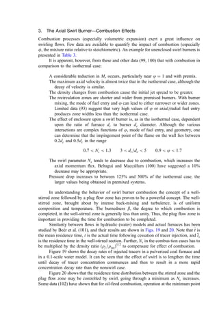
![Figure 6 Comparison of the predictions of Abramovich and Field et al. with the data of Syrkin and Lyakhousky on buoyant jet behavior. [From (13, 83, and 86).]](https://image.slidesharecdn.com/combustionandincinerationprocesses-220507104234-264c413a/85/COMBUSTION_AND_INCINERATION_PROCESSES-pdf-224-320.jpg)


![Abramovich (83) derived an analytical relation of the form
x
d0
¼
ffiffiffiffiffiffiffiffiffi
39
MCx
s
ln
10 þ y=d0 þ ½ðy=d0Þ2
þ 20ðy=d0Þ þ ð7=MCxÞ tan2
a01=2
10 þ
ffiffiffiffiffiffiffiffiffiffiffiffiffiffiffiffiffi
ð7=MCxÞ
p
tan a0
#
ð15Þ
where Cx is an effective drag coefficient relating drag on the jet to the momentum flux in
the external flow and has a value (dimensionless) of approximately 3.
A simplified treatment of jet behavior in crossflow with temperature effects was
presented by Davis (80) in 1937. The crossflow effect was introduced by the assumption
that the jet rapidly acquired a velocity component equal to the crossflow velocity. The jet
was then seen to follow a path corresponding to vector addition of the crossflow velocity to
the jet centerline velocity [the latter being calculated using a simplified velocity decay law
by Tollmien (90)]. Temperature effects were introduced as being reflected in increases in
jet velocity due to expansion of the cold nozzle fluid (initially at T0) after mixing with the
hot furnace gases (at Ta). Davis’ final equation for the deflection (y) is given by
y ¼
u1xðx þ 4d0 cos a0Þ
2a1d0
u
u0 cos2 a0
T0
Ta
1=3
þx tan a0 ð16Þ
where a1 is a constant depending on nozzle geometry (1.68 for round jets and 3.15 for
long, narrow plane jets). The many rough assumptions in Davis’ analysis (some of which
have been shown to be in error) would indicate that its use should be discouraged.
Comparison of calculated trajectories with observed flame contours (Fig. 4) suggests it
may have some general value. Interpretation of the meaning of the general agreement
between calculated jet trajectory and flame contour as shown in Fig. 4 is uncertain,
however, and use of the Davis equation in incinerator applications is questionable.
Patrick (87) reported the trajectory of the jet axis (defined by the maximum
concentration) to be
y
d0
¼ 1:0M1:25 x
d0
2:94
ða0 ¼ 0Þ ð17Þ
Figure 9 shows a plot of the velocity axis [Eq. (12)] and the concentration axis [Eq. (17)]
for a value of M ¼ 0:05. The concentration axis shows a larger deflection than does the
velocity axis. This is probably due, in part, to the asymmetry of the external flow around
the partially deflected jet. Also, recent calculations by Tatom (79) for plane jets suggest
that under crossflow conditions, streamlines of ambient fluid can be expected to cross the
jet velocity axis.
For our purposes, we are interested in jets that penetrate reasonably far into the
crossflow (i.e., those that have a relatively high velocity relative to the crossflow). The
empirical equations of Patrick (87) [Eq. (11)] and Ivanov (81) [Eq. (13)] were developed
from data that satisfy this condition. Figures 10 and 11 show comparisons of these two
equations for values of M of 0.001 (
u
u0=u1 ¼ 30) and 0.01 (
u
u0=u1 ¼ 10). Ivanov’s
expression predicts higher deflections at large x=d0 (particularly at M ¼ 0:01).
Ivanov (81) also investigated the effect of the spacing between jets (s) in a linear
array on jet trajectory. He measured the trajectories of jets under conditions where
M ¼ 0:01 for s ¼ 16, 8, and 4 jet diameters. His results are shown in Fig. 12 along
with the trajectory of a single jet (infinite spacing). The data show that reducing the
spacing between jets causes greater deflection of the jets. As spacing is reduced, the jets
tend to merge into a curtain. The blocking effect of the curtain impedes the flow of external](https://image.slidesharecdn.com/combustionandincinerationprocesses-220507104234-264c413a/85/COMBUSTION_AND_INCINERATION_PROCESSES-pdf-227-320.jpg)
![fluid around the jets and increases the effective deflecting force of the external fluid. The
increase in deflection is most notable as s=d0 is reduced from 16 to 8. Above s=d0 ¼ 16,
the merging of the jets apparently occurs sufficiently far from the nozzle mouth to have
little effect on the external flow. At s=d0 ¼ 8, the jet merge apparently takes place
sufficiently close to the nozzle mouth that further reduction in spacing has little added
effect.
Earlier data [Abramovich (83)] on water jets colored with dye issuing into a
confined, crossflowing stream were correlated in terms of jet penetration distance. The
penetration distance Lj was defined as the distance between the axis of the jet moving
parallel to the flow and the plane containing the nozzle mouth. The axis was defined as
being equidistant from the visible boundaries of the dyed jet. The resulting correlations
was
Lj
d0
¼ k
u
u0
u1
ð18Þ
Figure 9 Trajectory of concentration and velocity axes for jets in crossflow, M ¼ 0:05. [Data from
(87).]](https://image.slidesharecdn.com/combustionandincinerationprocesses-220507104234-264c413a/85/COMBUSTION_AND_INCINERATION_PROCESSES-pdf-228-320.jpg)
![where k is a coefficient depending on the angle of attack and the shape of the nozzle.
Defining the angle of attack d as the angle between the jet and the crossflow velocity
vectors and equal to (90 a0) in the terminology shown in Fig. 8, the recommended
values of k are presented in Table 2.
Figure 13 shows a comparison of Ivanov’s correlation [Eq. (13)] with the jet
penetration correlation [Eq. (18)] for M ¼ 0:001 and M ¼ 0:01.
Equation (18) predicts a smaller jet penetration than does Eq. (13). There are two
possible explanations for this discrepancy.
The data on which Eq. (13) was based do not extend to large values of x=d0, and
extrapolation of the data may be in error; and
The data on which Eq. (18) was based were taken in a confined crossflow in which
the lateral dimension (normal to both the jet axis and the crossflow) was
sufficiently small to interfere with normal jet spreading. The jet effectively
filled the cross-section in the lateral dimension, behaving like a series of jets at
low spacing.
Ivanov’s data (Fig. 12) show that penetration is reduced at lower spacing. The
penetration given in Eq. (13) for M ¼ 0:01 was reduced by 25% (see dotted trajectory
marked s=d0 ¼ 4, M ¼ 0:01 in Fig. 13). Agreement between this adjusted trajectory and
the penetration given by Eq. (18) is better.
d. Buoyancy and Crossflow. When a cold air jet is introduced into a cross-flowing
combustion chamber, both buoyancy and crossflow forces act simultaneously on the jet.
Figure 10 Comparison of trajectories at M ¼ 0:001 (u0=u1 ¼ 31:6) for jets in crossflow.](https://image.slidesharecdn.com/combustionandincinerationprocesses-220507104234-264c413a/85/COMBUSTION_AND_INCINERATION_PROCESSES-pdf-229-320.jpg)
![when the value of M was computed using actual fluid densities. From these data,
Abramovich concluded that buoyancy effects could be neglected, other than as density
differences were incorporated into the crossflow parameter M.
The same conclusion was drawn by Ivanov (81) it who injected hot jets into a cold
crossflow. The ratio of temperature (and density) between jet and ambient fluids was 1.9,
and M ranged from 0.005 to 0.02. The geometry of the tests was not clearly stated by
either Abramovich or Ivanov. It appears that the buoyancy force acted in the same direction
as the crossflow force in Ivanov’s tests (i.e., a hot jet discharging into an upflow).
Application of these conclusions to incinerator design practice, however, is subject
to question because of the large geometrical scale-up involved. Physical reasoning
suggests that the ratio of buoyant force to drag force acting on a nonisothermal jet in
crossflow depends on scale. The buoyant force Fb is a body force and is, therefore,
Figure 12 Effect of jet spacing on trajectory for jets in crossflow. [After (81).]](https://image.slidesharecdn.com/combustionandincinerationprocesses-220507104234-264c413a/85/COMBUSTION_AND_INCINERATION_PROCESSES-pdf-231-320.jpg)
![proportional to jet volume. The drag force Fd exerted by the crossflow has the
characteristics of a surface force and is, therefore, proportional to the effective cylindrical
area of the jet. Therefore, the ratio of buoyant force to drag force is proportional to jet
diameter. A simple analysis, discussed in (63), gives
Fb
Fd
¼
p
2Cx
gd0
u2
1
1
r0
ra
ð19Þ
where Cx is the effective drag coefficient.
The value of the effective drag coefficient Cx is believed to be in the range of 1 to 5;
analysis given in (63) suggests that 4.75 is an acceptable value.
Typical values of the physical parameters in Ivanov’s experiments (81) are
d0 ¼ 5 to 20 mm
u
u0=u1 ¼ 10 to 20
T0=Ta ¼ ra=r0 ¼ 2
r0
u
u2
0=rau2
1 ¼ 100 to 200
u1 ¼ 3:68 to 4:16 m=sec
Figure 13 Comparison of Ivanov’s trajectory correlation (Eq. 13) with jet penetration correlation
(Eq. 18). [From (81).]](https://image.slidesharecdn.com/combustionandincinerationprocesses-220507104234-264c413a/85/COMBUSTION_AND_INCINERATION_PROCESSES-pdf-232-320.jpg)


![For the oxygen-rich case, if Tm Ti and if yð1 OÞ Oc0 0, combustion will
occur to the extent of the available fuel, releasing DHcð1 OÞ kcal=kg of mixture. The
resulting gas temperature is given by
TF ¼ TR þ
1
c
p;av
½ð1 OÞðT1 TRÞc
p;av þ DHcð1 OÞ ð29Þ
Calculation of the radial profiles of temperature according to the above was carried out,
and the results are plotted in Figs. 14, 15, and 16, at various distances from the nozzle
plane. The depressed temperature (600
C) near the discharge plane is the subignition
temperature or ‘‘quenched’’ region. The peaks of temperature found along a radial
temperature ‘‘traverse’’ identify the stoichiometric point. The peak temperature (about
1400
C) reflects the assumptions
Ta ¼ 1094
C (2000
F)
DHc ¼ 206 kcal=kg (370 Btu=lb)
y ¼ 0:0545 kg O2=kg ambient
c
c0 ¼ 0:23 kg O2=kg nozzle fluid (air)
c
p;av ¼ 0:31 kcal=kg
C1
relative to 15.5
C
Note that only absolute temperatures are to be substituted in the equations.
It can be seen that a hot zone is rapidly developed with a diameter of about 30 cm
(1 ft) and this zone endures, for large jets, for distances that approximate the widths of
many incinerator furnaces (2 to 3 m). This problem is greatly reduced as the jet diameter is
decreased, thus adding additional incentive to the use of small-diameter jets.
The rapid attainment of stoichiometric mixtures within the jet is in agreement with
the theory developed by Thring (92), which roughly approximates the spread in velocity
and concentration using the same mathematical formulations as in Eqs. (1) through (4), but
Figure 14 Temperature versus radial distance (jet diameter ¼ 1:5 in.). [From (63).]](https://image.slidesharecdn.com/combustionandincinerationprocesses-220507104234-264c413a/85/COMBUSTION_AND_INCINERATION_PROCESSES-pdf-238-320.jpg)
![using an effective nozzle diameter equal to d0ðr0=rf Þ1=2
, where rf is the gas density at the
temperature of the flame.
The above illustrates the characteristics of ‘‘blowtorch’’ effects from air jets and
shows that temperatures near 1400
C, such as have been experienced with jets, could be
anticipated. However, the quantitative accuracy of the above calculations is limited to
Figure 15 Temperature versus radial distance (jet diameter ¼ 2 in.). [From (63).]
Figure 16 Temperature versus radial distance (jet diameter ¼ 4 in.). [From (63).]](https://image.slidesharecdn.com/combustionandincinerationprocesses-220507104234-264c413a/85/COMBUSTION_AND_INCINERATION_PROCESSES-pdf-239-320.jpg)
![(neglecting combustion) suggests jet drop will be important, these effects could provide
counterbalancing jet temperature increases.
g. Incinerator Overfire Air Jet Design Method. The basic parameters to be selected in
design of an overfire air jet system are
The diameter (d0) and number (N) of the jets to be used
The placement of the jets
The quantity of the air to be added over the fire
Related but not independent variables are the jet velocity
u
u0 and the head
requirements for the overfire air fan P.
The tentative design method is based on that of Ivanov (81), which was discussed
above. It is important in using this method to substitute the values of d0 and u1 obtained
into Eq. (19) to determine if buoyant forces might be important. Values should fall in the
‘‘drag forces’’ predominate region.
The basic equations on which the design method is based are as follows:
Air Flow Relation
QT ¼ 47Nd2
0
u
u0 ð36Þ
where
QT ¼ the overfire air rate (m3
=min)
N ¼ the number of jets
d0 ¼ the jet diameter (m)
u
u0 ¼ the jet velocity (m=sec)
Ivanov’s Penetration Equation
Lj
d0
¼ 1:6
u
u0
u1
ffiffiffiffiffi
r0
ra
r
ð37Þ
where
Lj ¼ the desired jet penetration
u1 ¼ the estimated crossflow velocity in the incinerator
r0 and ra ¼ the jet and crossflow gas densities, respectively
Jet Spacing Equation
z ¼
s
d0
Nd0 ð38Þ
where
z ¼ the length of furnace wall on which the jets are to be placed
s=d0 ¼ the desired value of jet spacing (measured in jet diameters)
Inherent in Eq. (38) is the assumption that the jets are placed in a single line. Ivanov
recommends that s=d0 be in the range of 4 to 5, although values as low as 3 can probably
be used without invalidating the penetration equation [Eq. (37)].](https://image.slidesharecdn.com/combustionandincinerationprocesses-220507104234-264c413a/85/COMBUSTION_AND_INCINERATION_PROCESSES-pdf-241-320.jpg)

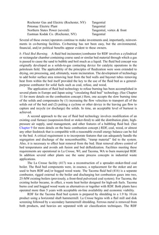
![ð99:4=425Þð100Þ ¼ 23% of theoretical. The soundness of this value can be
checked by comparison with the air requirements defined by the bed-burning
process and by reference to experience. Note, however, that few data exist to
allow confident valuation of the performance of existing plants with respect to
combustible pollutant emissions and the design and operating parameters of the
overfire air systems.
The amount of overfire air can be increased or decreased within limits without
seriously affecting the performance of the jets by changing the jet spacing parameter [s=d0
in Eq. (38)] within the range of 3 to 5. It should be recognized that the design method
described has as its goal the complete mixing of fuel vapors arising from the fuel bed with
sufficient air to complete combustion. Two other criteria may lead to the addition of
supplementary air quantities: the provision of sufficient secondary air to meet the
combustion air requirement of the fuel vapors, and the provision of sufficient air to
temper furnace temperatures to avoid slagging (especially in refractory-lined incinerators).
In the example given, both criteria act to greatly increase the air requirement and would
suggest the installation of additional jets (although the discharge velocity criteria are
relaxed). Nonetheless, the Ivanov method is intended to ensure the effective utilization of
overfire air and, in boiler-type incinerators where tempering is not required, will permit
optimal design and operating efficiency.
h. Isothermal Slot Jets. The discussions above have dealt with the round jet, the
configuration found almost exclusively in combustion systems. In designs where a
multiplicity of closely spaced round jets are used, however, the flow fields of adjacent
jets merge. The flow then takes on many of the characteristics of a jet formed by a long slot
of width y0.
For use in analyzing such situations, the flow equations applicable to such a slot jet
(or plane jet) are as follows.
Centerline velocity:
u
um
u
u0
¼ 2:48
x
y0
þ 0:6
1=2
r0
ra
1=2
ð43Þ
Centerline concentration:
c
cm
c
c0
¼ 2:00
x
y0
þ 0:6
1=2
r0
ra
1=2
ð44Þ
Transverse velocity:
u
u
u
um
¼ exp 75
y
x
2
ð45aÞ
¼ 0:5 1 þ cos
py
0:192x
h i
ð45bÞ
Transverse concentration:
c
c
c
cm
¼ exp 36:6
y
x
2
ð46aÞ
¼ 0:5 1 þ cos
py
0:279x
h i
ð46bÞ](https://image.slidesharecdn.com/combustionandincinerationprocesses-220507104234-264c413a/85/COMBUSTION_AND_INCINERATION_PROCESSES-pdf-243-320.jpg)


![Figure 17 (a) Inlet losses for various types of swirlers. (b) Chamber-friction, swirl, and outlet
losses. [From (97).]
Figure 18 Dependence of the aerodynamic efficiency on the constructional parameters of Type A
cyclone combustors. Points obtained from tests on eight different cyclones in self-similarity
Reynolds number range (Re 50,000) by Tager. [From (97).]](https://image.slidesharecdn.com/combustionandincinerationprocesses-220507104234-264c413a/85/COMBUSTION_AND_INCINERATION_PROCESSES-pdf-247-320.jpg)


![in well-stirred residence time yields maximum performance with minimum smoke
emissions.
4. The Cyclone Combustion Chamber—Combustion Effects
Data on cyclone systems with combustion are few; this is due, importantly, to the
experimental difficulties encountered with the high-ash or slagging fuels most often
fired in this type of equipment. Some conclusions, however, can be drawn:
Figure 19 Tracer concentration decay as a function of swirl number in model and prototype
furnace. [From (101).]](https://image.slidesharecdn.com/combustionandincinerationprocesses-220507104234-264c413a/85/COMBUSTION_AND_INCINERATION_PROCESSES-pdf-252-320.jpg)
![Optimum combustion can be obtained by admitting 2% to 3% of the combustion air
on the axis. Axial introduction of fuel leads to incomplete mixing and poor
combustion.
At least two symmetrically arranged tangential inlets should be used to avoid uneven
burning and excessive pressure drop.
In combustion situations, up to three major zones of oxygen deficiency occur, one
commonly occurring in the region of the exit throat. This phenomenon, perhaps
due in part to centrifugal stratification effects, leads to the need for an after-
burning chamber to obtain complete burnout.
Comparisons between isothermal and combusting system regarding flow pattern and
pressure drop show strong similarity. For evaluating Ns in the combusting state,
the following correction is recommended:
ðNsÞcombusting ¼ ðNsÞisothermal
Tinlet
K
Toutlet
K
ð59Þ
II. INDUCED FLOW
For the combustion systems and subsystems described above, emphasis was placed on the
flow elements directly within the control of the designer, the axial and sidewall jet and the
swirled jet or cyclonic flow. This section explores the consequential effects of these flows
(recirculation) and the impact of buoyancy forces on furnace flow. Each of these induced
Figure 20 Ratio of residence time in stirred section to total residence time as a function of swirl
number. [From (101)]](https://image.slidesharecdn.com/combustionandincinerationprocesses-220507104234-264c413a/85/COMBUSTION_AND_INCINERATION_PROCESSES-pdf-253-320.jpg)
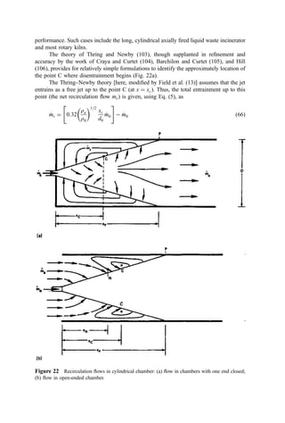

![performance. Such cases include the long, cylindrical axially fired liquid waste incinerator
and most rotary kilns.
The theory of Thring and Newby (103), though supplanted in refinement and
accuracy by the work of Craya and Curtet (104), Barchilon and Curtet (105), and Hill
(106), provides for relatively simple formulations to identify the approximately location of
the point C where disentrainment begins (Fig. 22a).
The Thring–Newby theory [here, modified by Field et al. (13)] assumes that the jet
entrains as a free jet up to the point C (at x ¼ xc). Thus, the total entrainment up to this
point (the net recirculation flow mr) is given, using Eq. (5), as
_
m
mr ¼ 0:32
ra
r0
1=2
xc
d0
_
m
m0
#
_
m
m0 ð66Þ
Figure 22 Recirculation flows in cylindrical chamber: (a) flow in chambers with one end closed;
(b) flow in open-ended chamber.](https://image.slidesharecdn.com/combustionandincinerationprocesses-220507104234-264c413a/85/COMBUSTION_AND_INCINERATION_PROCESSES-pdf-257-320.jpg)
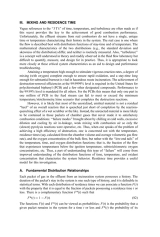

![4. General Case
Wolf and Resnick (421) considered the general case where one was analyzing experimental
data in an evaluation of a system comprised of a mixture of plug flow and perfect mixing
with dead zones and short-circuiting. Their consideration included the effects of uncer-
tainties in the calculated residence time due to experimental errors and, in addition, lag
times between actual effluent gas composition changes and reported changes (e.g., as
through holdup in sampling lines). Their assessment of the resulting F function was given
by
FðtÞ ¼ 1 eZ xðe=y
½ Þ
FðtÞ 0 ð91Þ
The term Z can be considered as a measure of the efficiency of mixing: equal to unity for
perfect mixing and approaching infinity for the plug flow case. Dead space also results in Z
greater than unity. Short-circuiting results in Z less than unity. Errors in the evaluation of
the average residence time could make Z greater than or less than unity.
The term e is a measure of the phase shift in the system. If e=y 0 (the case for plug
flow or a system lag), the system response lags behind that expected for perfect mixing.
Short-circuiting gives a negative value for e.
If one analyzes reported residence time distributions for single-stage systems, one
finds that the data can be replotted as ln½1 FðtÞ vs. x to yield a straight line. Then Z and e
can be determined from the slope and intercept. Note, however, that behavior inferred from
Figure 23 Perfect mixing with plug flow. [From (421)]](https://image.slidesharecdn.com/combustionandincinerationprocesses-220507104234-264c413a/85/COMBUSTION_AND_INCINERATION_PROCESSES-pdf-264-320.jpg)
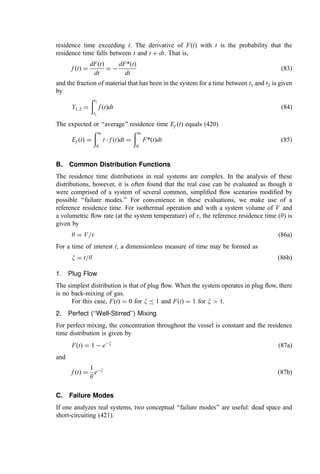
![Figure 24 Perfect mixing with dead space. [From (421).]
Figure 25 Perfect mixing with short circuit. [From (421).]](https://image.slidesharecdn.com/combustionandincinerationprocesses-220507104234-264c413a/85/COMBUSTION_AND_INCINERATION_PROCESSES-pdf-265-320.jpg)


![To calculate the pressure drop for steady flow, two dimensionless numbers are used:
a modified Reynold’s number given by
N0
Re ¼
r0u0d0
Z0
¼
d0G
Z0
ð12Þ
and the Hedstrom number NHe (the product of the Reynold’s number and the ratio of the
yield stress to the viscous force) as given by
NHe ¼
d2
0 t0gcr0
Z2
0
ð13Þ
Equation (9) can be used to estimate the pressure drop DP in atm for r0 in kg=m3
, the
length L in m, the velocity V in m=sec, and using Z0 in centipoise as the Bingham plastic
limiting value (at high shear rate) for the coefficient of rigidity. The overall Fanning
friction factor ( f ) in Eq. (9) should be developed (207) as a function of the friction factor
for laminar ( fL) and turbulent ( fT ) flow by:
f ¼ ð f b
L þ f b
T Þ1=b
ð14Þ
where fL is the (iterative) solution to Eq. (15):
fL ¼ ½16=NRe0 ½1 þ ð1=6ÞðNHe=NRe0 Þ ð1=3ÞðN4
He=f 3
N7
Re0 Þ ð15Þ
Figure 3 Viscometer test of sewage sludge. (From [223]).](https://image.slidesharecdn.com/combustionandincinerationprocesses-220507104234-264c413a/85/COMBUSTION_AND_INCINERATION_PROCESSES-pdf-287-320.jpg)
![with
fT ¼ 10a
N0:193
Re0 ð14Þ
and where
a ¼ 1:47½1:0 þ 0:146 expð2:9 105
NHeÞ ð15Þ
and
b ¼ 1:7 þ 40;000=NRe0 ð16Þ
An estimate of the friction factor can also be taken from Fig. 5.
Figure 5 Friction factor for sludge analyzed as a Bingham plastic. (From [223]).
Figure 4 Comparison of behaviors of wastewater sludge and water flowing in circular pipelines.
(From [223]).](https://image.slidesharecdn.com/combustionandincinerationprocesses-220507104234-264c413a/85/COMBUSTION_AND_INCINERATION_PROCESSES-pdf-288-320.jpg)


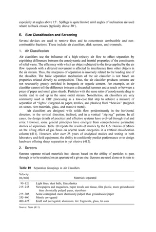
![The fine ash that has no salvage value is usually transported by truck to a residue
disposal site. Because the fine ash is often enriched with heavy metals, these residues are
usually segregated within the landfill in a separate cell (a ‘‘monofill). This minimizes the
potential leaching of metals occasioned by percolation through the residue mass of organic
acids formed as a normal product of the biological breakdown of refuse within the landfill.
3. Vitrification
The several tables presented above indicate that incinerator residue contains relatively high
concentrations of heavy metals and that the leaching of these metals from the residue is,
for some regulatory agencies, a matter of concern. Over long times, leaching will occur
and, if the residue is not placed in landfills with adequate leachate control and treatment
systems, there is a potential for groundwater contamination. In the United States and in
some other countries, the legal liability of the groundwater contamination resides with the
waste generator (here, the incinerator operator) even though many years may have passed.
All of these problems and the general problem of finding acceptable disposal sites for
residue have led some jurisdictions to vitrify (melt) the residue to a glass. In the vitrifier,
the residue is heated to the fusion point whereupon metals are bound into the matrix of the
glass and rendered substantially insoluble. Residue processing by vitrification allows use
of the residue as an aggregate or as a ‘‘clean fill’’ without concern regarding environmental
contamination impacts.
Vitrification technology has been studied in several countries but is primarily
practiced in Japan [see (467) and the Kubota furnace described in Section 3.A in Chapter
9]. In Japan, environmental concerns coupled with extreme cost and siting difficulties for
landfills encourage consideration and, in some cases, implementation of vitrification
schemes. Vitrification technologies involve use of electric arc furnaces, high-temperature
combustion, and other means to raise the residue temperature to above 1500
C. In some
instances, lime is added to modify the melting temperature. Under most circumstances, the
cost for vitrification equipment and the expense of purchased energy to effect vitrification
far exceed the cost of landfill disposal options.
4. Financial Considerations in Residue Processing
Residue is usually not regarded as an incineration by-product of great quality or worth. Its
variable properties generally make its use in high-specification products impossible. In
most cases, the residue must be transported (another cost) to another location for use.
Table 11 Granulometry of Certified Municipal Solid Waste Bottom Ash
Roadbase material Roadbase material
Coarse type (0=20) unbonded (0=20) cement bonded Embankment material
on sieve % (m=m) % (m=m) (0=40)
45 mm 0 nil 0–10
22.4 mm 0–10 0–10 nil
8 mm 10–40 10–40 nil
2 mm 40–70 40–70 nil
63 mm 92–100 nil 92–100
Source: From (463).](https://image.slidesharecdn.com/combustionandincinerationprocesses-220507104234-264c413a/85/COMBUSTION_AND_INCINERATION_PROCESSES-pdf-345-320.jpg)

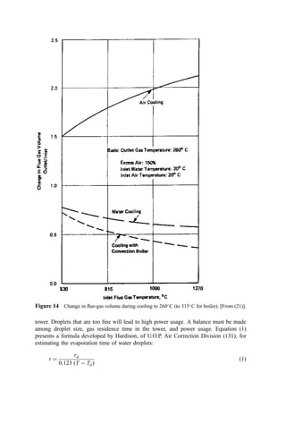

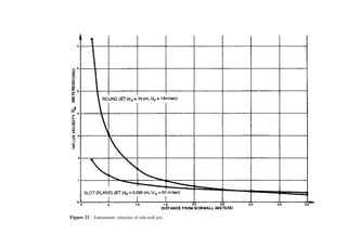
![tower. Droplets that are too fine will lead to high power usage. A balance must be made
among droplet size, gas residence time in the tower, and power usage. Equation (1)
presents a formula developed by Hardison, of U.O.P. Air Correction Division (131), for
estimating the evaporation time of water droplets:
t ¼
rd
0:123 ðT TdÞ
ð1Þ
Figure 14 Change in flue-gas volume during cooling to 260
C (to 315
C for boiler). [From (21)].](https://image.slidesharecdn.com/combustionandincinerationprocesses-220507104234-264c413a/85/COMBUSTION_AND_INCINERATION_PROCESSES-pdf-349-320.jpg)
![where
t ¼ residence time in sec
rd ¼ droplet radius in microns
T ¼ temperature of gas ð
CÞ
Td ¼ temperature of droplet ð
CÞ
A second and more complex method of estimating (in a step-wise fashion) the evaporation
time of droplets (up to about 600 mmÞ uses the graph shown in Fig. 15, where
Ta ¼ gas temperature ðKÞ
DT ¼ Ta 54 ð
CÞ
m ¼ gas viscosity at Ta ðg cm1
sec1
Þ
b ¼ 0:071 ðm2
TaÞ0:36
If the drop temperature varies significantly from 54
C, the evaporation time may be
corrected by a factor (Ta 54Þ=ðTa TdropÞ. It is suggested that users of this latter method
consult the original paper (132).
Although both of these methods are useful in estimating the residence time required
for evaporation, care must be taken in selecting a nozzle that provides uniform-size
droplets rather than droplets with a wide size distribution, since the largest droplet will
dictate the length of the conditioning tower.
Figure 15 Theoretical evaporation time for water droplets in hot gas streams. [From (132)].](https://image.slidesharecdn.com/combustionandincinerationprocesses-220507104234-264c413a/85/COMBUSTION_AND_INCINERATION_PROCESSES-pdf-350-320.jpg)
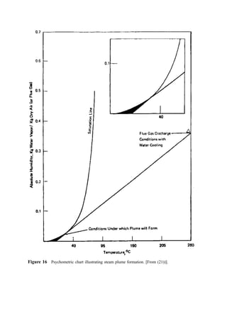

![Figure 16 Psychometric chart illustrating steam plume formation. [From (21))].](https://image.slidesharecdn.com/combustionandincinerationprocesses-220507104234-264c413a/85/COMBUSTION_AND_INCINERATION_PROCESSES-pdf-353-320.jpg)


![often added to the ignition tile, increasing the intensity of radiation (for waste vaporiza-
tion). When wastes contain a substantial fusible ash content, special care must be given to
the type and design of these tiles to avoid rapid fluxing losses and slag buildup.
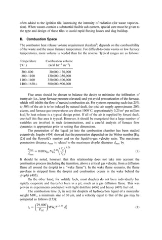
D. Combustion Space
The combustor heat release volume requirement (kcal=m3
) depends on the combustibility
of the waste and the mean furnace temperature. For difficult-to-burn wastes or low furnace
temperatures, more volume is needed than for the reverse. Typical ranges are as follows:
Temperature Combustion volume
(
C ) (kcal hr1
m3
)
300–800 30,000–130,000
800–1100 130,000–350,000
1100–1400 350,000–500,000
1400–1650þ 500,000–900,000
Flue areas should be chosen to balance the desire to minimize the infiltration of
tramp air (i.e., keep furnace pressure elevated) and yet avoid pressurization of the furnace,
which will inhibit the flow of needed combustion air. For systems operating such that 25%
to 50% of the air is to be induced by natural draft, the total air supply approximates 20%
excess, and furnace gas temperatures are about 1000
C; approximately 0.25 m2
per million
kcal=hr heat release is a typical design point. If all of the air is supplied by forced draft,
one-half this flue area is typical. However, it should be recognized that a large number of
variables are involved in such determinations, and a careful analysis of furnace flow
dynamics is appropriate prior to setting flue dimensions.
The penetration of the liquid jet into the combustion chamber has been studied
extensively. Ingebo (404) showed that the penetration depended on the Weber number [Eq.
(2)] and the Reynold’s number and on the liquid-to-gas velocity ratio. The maximum
penetration distance xmax is related to the maximum droplet diameter dmax by
xmax
dmax
¼ 0:08NRe N0:41
We
Vg
VL
0:29
ð7Þ
It should be noted, however, that this relationship does not take into account the
combustion process (including the transition, above a critical gas velocity, from a diffusion
flame all around the droplet to a ‘‘wake flame’’). In the wake flame scenario, the flame
envelope is stripped from the droplet and combustion occurs in the wake behind the
droplet (405).
On the other hand, for volatile fuels, most droplets do not burn individually but
rapidly evaporate and thereafter burn in a jet, much as a gas diffusion flame. This was
proven in experiments conducted with light distillate (406) and heavy (407) fuel oil.
The combustion time (tb in sec) for droplets of hydrocarbon liquid of a molecular
weight MWi, a minimum size of 30 mm, and a velocity equal to that of the gas may be
computed as follows (153):
tb ¼
29;800
PO2
MWiT1:75
d2
0 ð8Þ](https://image.slidesharecdn.com/combustionandincinerationprocesses-220507104234-264c413a/85/COMBUSTION_AND_INCINERATION_PROCESSES-pdf-433-320.jpg)


![packing can be held at high temperatures for an extended time to burn out (‘‘bake out’’)
accumulated organic particulate matter. The effectiveness of the seal on the gas valves and
the disposition of the gases in the internal gas passages in the RTO are important
parameters when the DRE requirements for the RTO exceed 95%. Leaking valves
obviously lead to the bypassing of unremediated gases from the inlet plenum to the
outlet duct. The redirection of the incoming gas in the ducting to the outlet duct within the
RTO during switchover also could result in the avoidance of the combustion zone. To
avoid this, manufacturers purge the unremediated gas before opening the valve to the
outlet duct.
B. Current Afterburner Engineering Technology
A large body of knowledge, both theoretical and empirical, is available to support and
guide the design and evaluation of afterburner systems. This knowledge, which concerns
the heat transfer, fluid mechanics, and kinematics of combustion phenomena, can be used
to determine the design characteristics for optimum performance and thus to develop
criteria against which to evaluate existing afterburner systems.
1. Direct Flame Afterburner Technology
Considerable experience exists in the use of direct flame afterburners for the combustion of
gaseous and gas-borne combustible pollutants (152,153). Many of these systems consist of
little more than a burner in a cylindrical, refractory-lined chamber and are constructed on-
site by facilities engineers. Indeed, the designs of many direct flame afterburners now on
the market are derived from such ‘‘homemade’’ devices.
a. Combustible Gaseous Pollutant Control. Most applications for afterburners concern
the destruction of combustible gaseous emissions and, particularly, volatile organic
compounds (VOCs). The concentration of these pollutants is usually too low to permit
self-sustaining combustion because they are often intentionally diluted below the lower
flammability limit for safety reasons. As a result, external energy must usually be added.
Most insurance carriers insist that the gases entering the incinerator be below 25% of the
lower explosive limit (LEL) [which can be estimated, for gas mixtures (298) using Eq. (9)].
For the LEL of pure substances, see Appendix D.
LELmix ¼
1
Pn
j
xj
ð
Pn
i xiÞ LELj
ð9Þ
where
LELmix ¼ lower explosive limit of a mixture of n components
xi; xj ¼ volume fraction of combustible components i; j
LEL ¼ lower explosive limit of component j
The energy content equivalent to the lower limit of flammability of most gas–air
mixtures is 0.46 kcal=Nm3
; therefore, fuel must be introduced into the gas stream to
increase the energy potential and permit subsequent ignition and oxidation of the mixture.
Because preheat (sensible energy) in the pollutant stream is equivalent to chemical energy,
the flammability energy limit (kcal=Nm3
) decreases as the inlet temperature increases until
it is zero at the ignition temperature.](https://image.slidesharecdn.com/combustionandincinerationprocesses-220507104234-264c413a/85/COMBUSTION_AND_INCINERATION_PROCESSES-pdf-437-320.jpg)
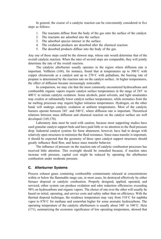


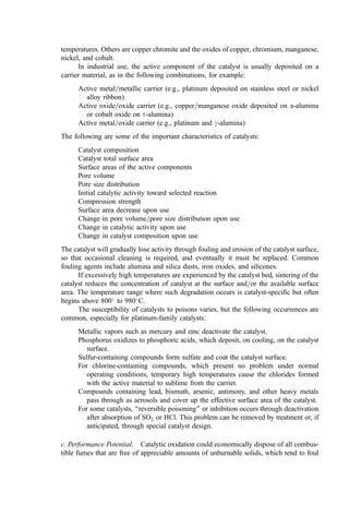
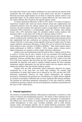


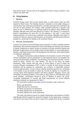
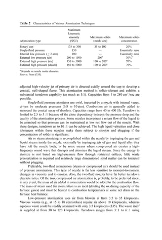

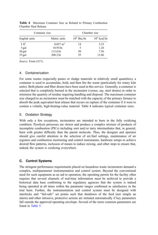
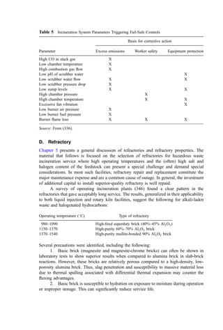
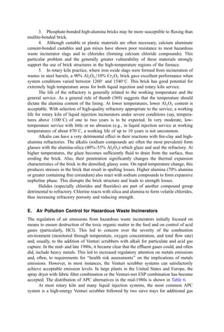


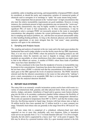
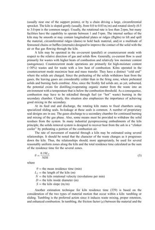


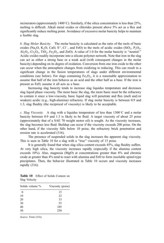

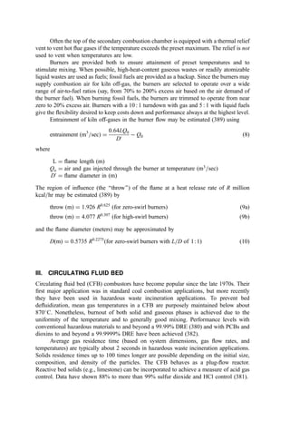
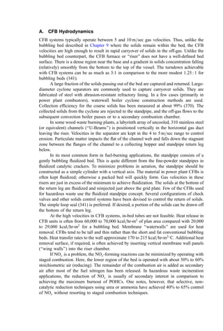


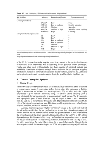
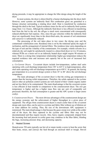


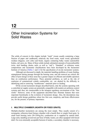
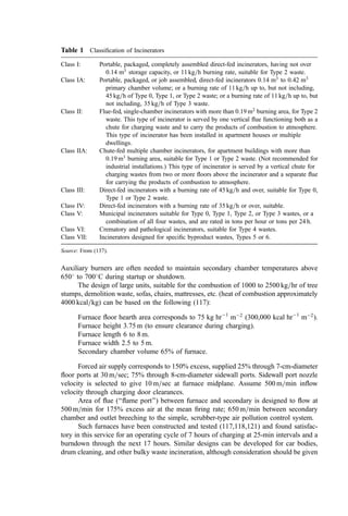

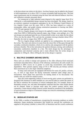

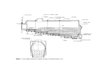

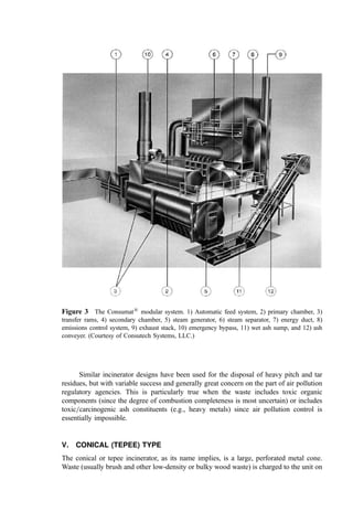
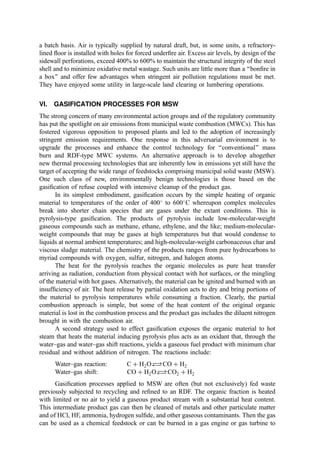
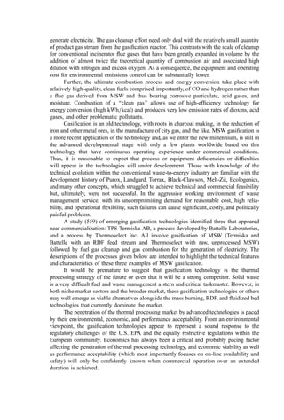


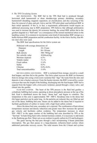


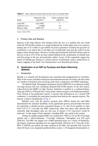


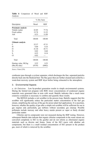


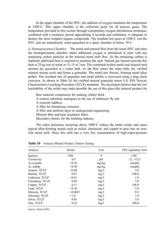


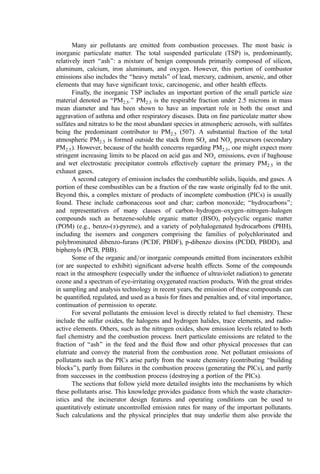
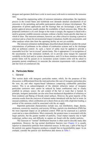
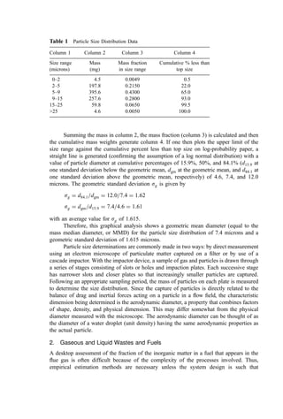

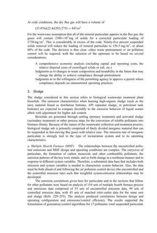


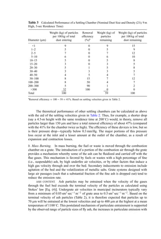
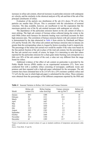
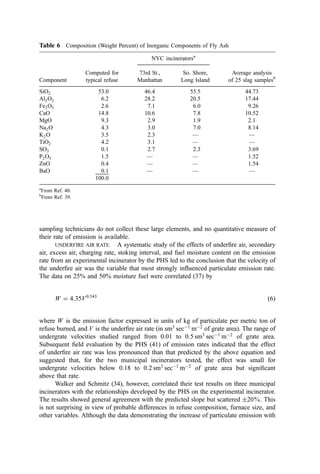
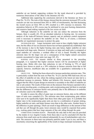

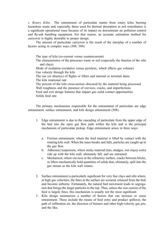
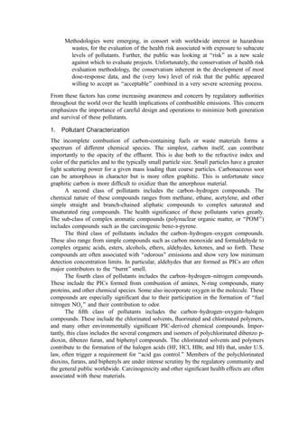


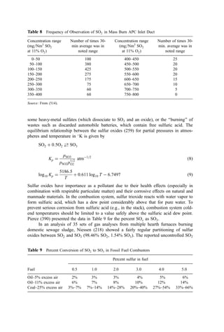
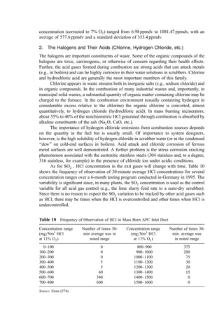
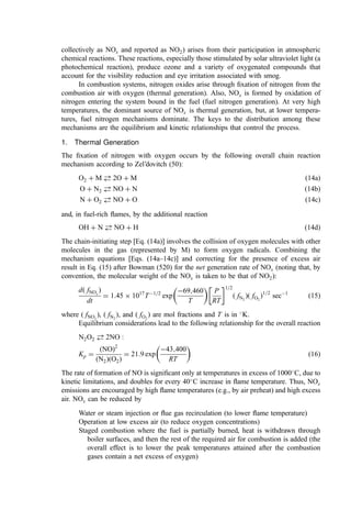


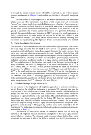

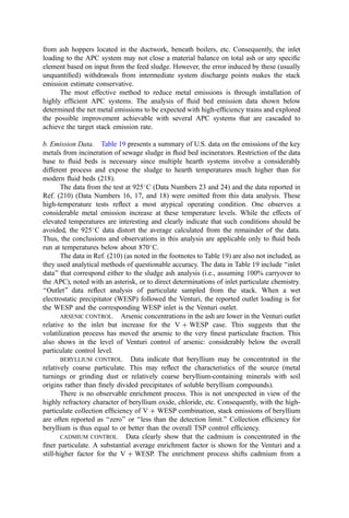

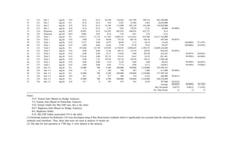

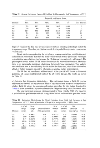

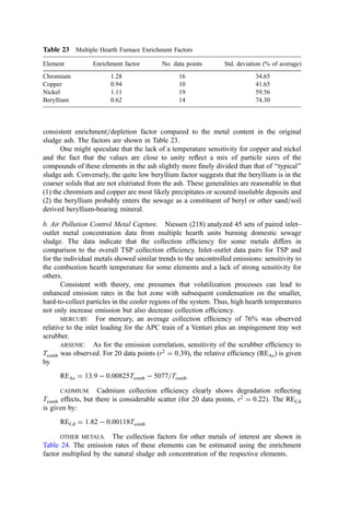


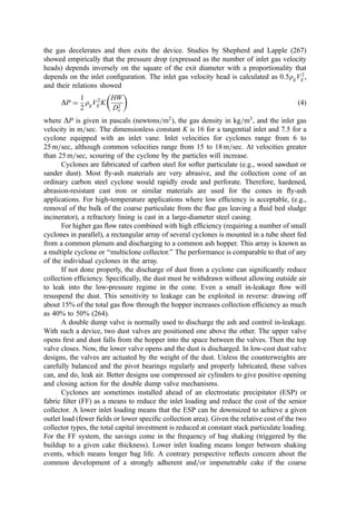

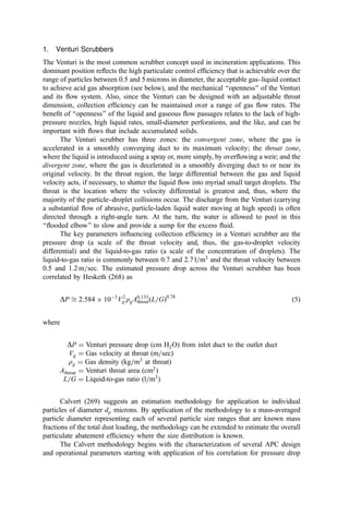


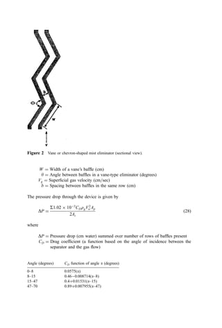
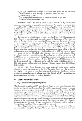
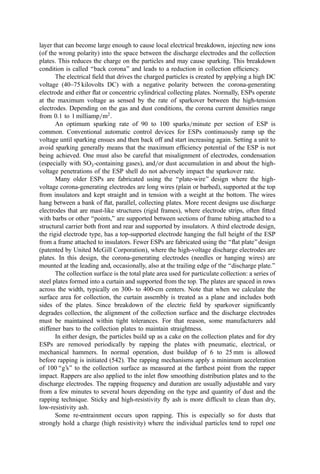


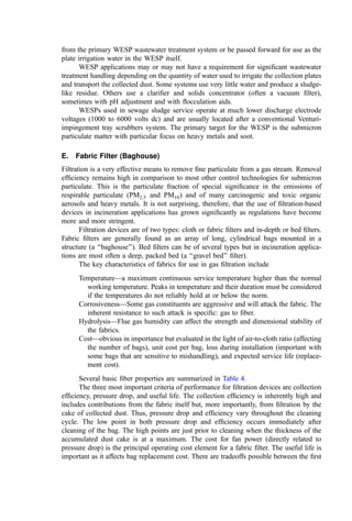

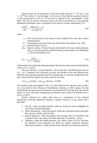
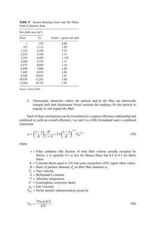


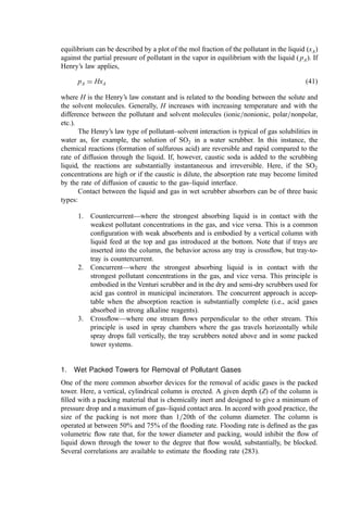


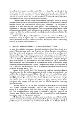


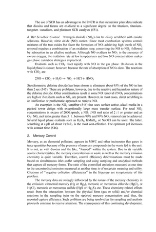

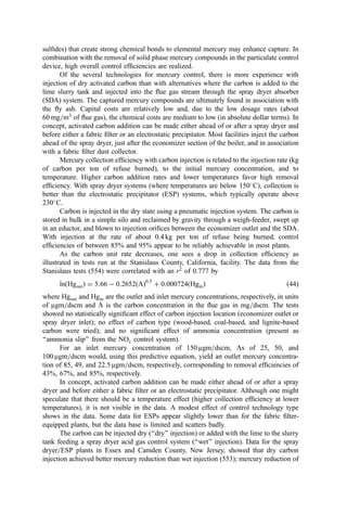
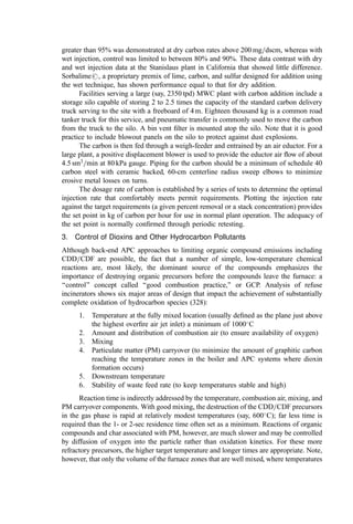

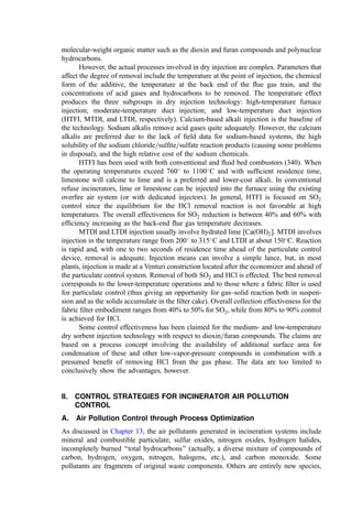


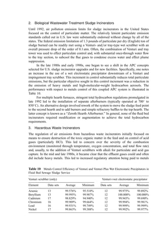
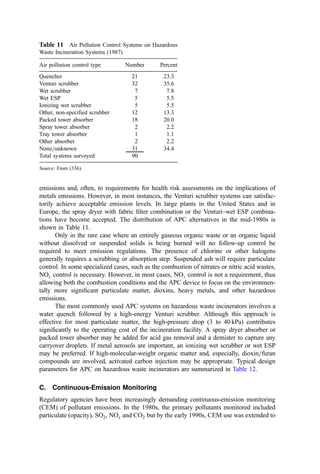
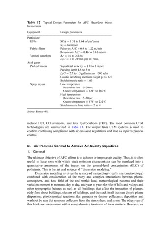
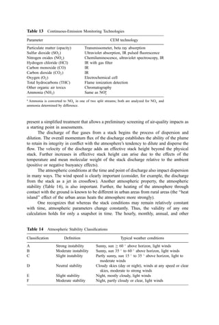


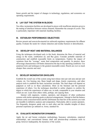

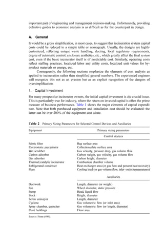


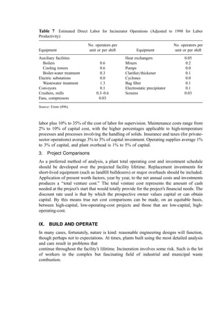


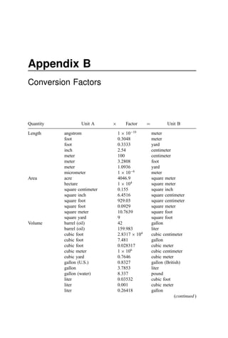

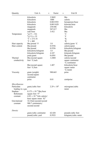

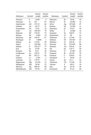
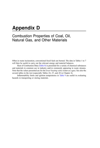
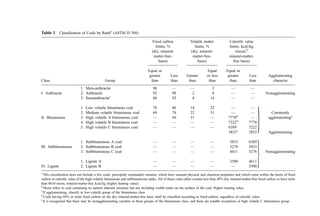
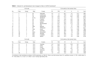
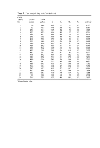

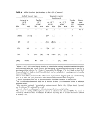


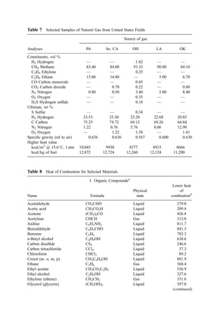

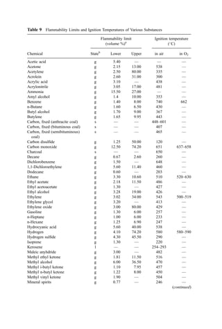


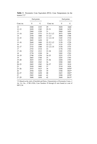


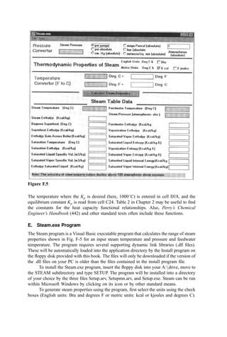


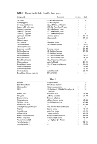


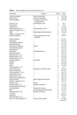
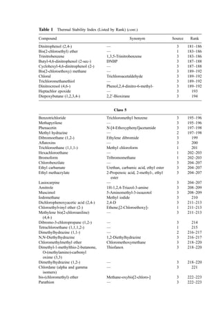


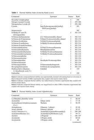

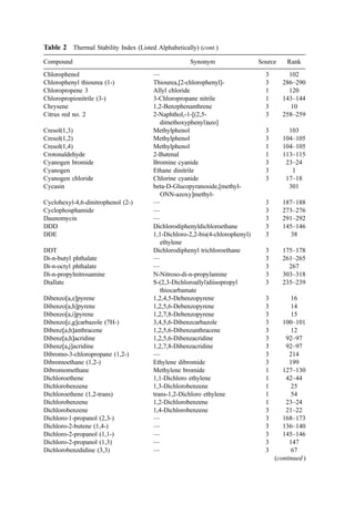

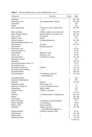
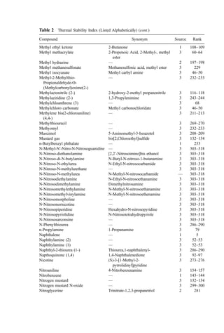
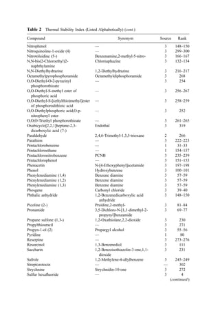
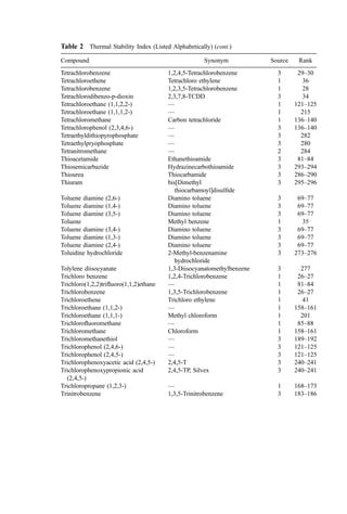


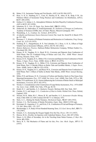


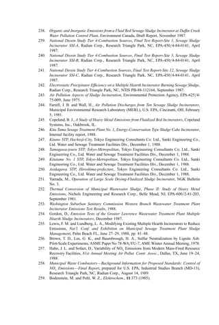

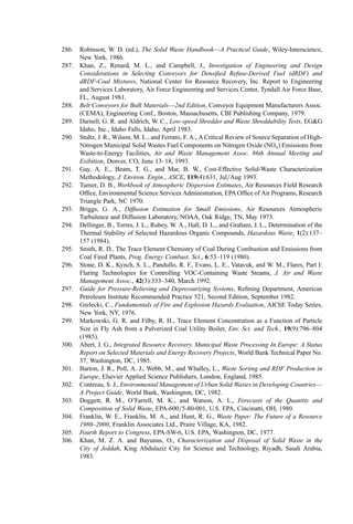
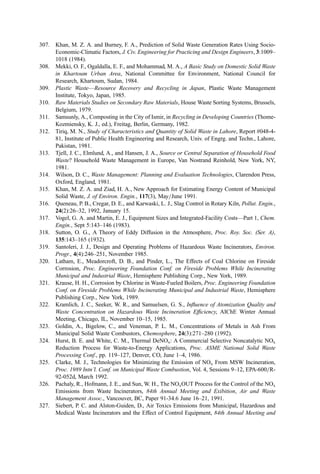


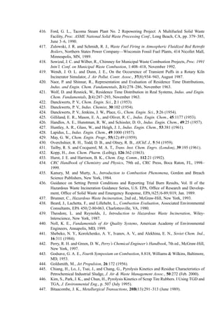


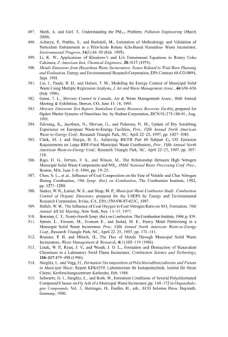


This document provides a summary of the third edition of the book "Combustion and Incineration Processes" by Walter R. Niessen. The third edition has been revised and expanded with new information on combustion, air pollution control, process evaluation, and incineration system design and operation from the 1990s. It also covers additional details on municipal waste incineration, alternative gasification technologies, lower-temperature soil remediation, and plasma waste treatment. The accompanying diskette provides additional computer tools. The introduction expresses that incineration faced increased regulation and public opposition in the US in the 1990s, while many European nations increased support for incineration to meet waste disposal restrictions. The book aims to help


