BOHR International Journal of Smart Computing
and Information Technology
2022, Vol. 3, No. 1, pp. 43–49
DOI: 10.54646/bijscit.2022.26
www.bohrpub.com
REVIEW
CNN-based plastic waste detection system
Grourou Aya Aridj1, Louchen Saher1 and Guezouli Larbi2*
1University of Batna 2, Batna, Algeria
2LEREESI, Higher National School of Renewable Energies, Environment and Sustainable Development, Batna, Algeria
*Correspondence:
Guezouli Larbi,
larbi.guezouli@hns-re2sd.dz
Received: 18 June 2022; Accepted: 08 July 2022; Published: 30 July 2022
Plastic waste has become a pressing global concern in recent decades, posing significant challenges to our
environment due to its non-biodegradable nature and causing significant pollution and damage to our planet.
Recycling plastic waste is one of the most effective solutions to this dilemma, which is why the aim of our project
was to create a system that detects plastic waste using a large dataset with labeled data and one of the most
famous deep learning neural networks, “Convolutional Neural Networks,” to classify and speed up the waste
collection process and provide an easier recycling process. Thanks to our work, we have achieved 97% accuracy.
Keywords: plastic waste detection, Convolutional Neural Networks (CNN), deep learning (DL), real-time, waste
management
Introduction
Plastic waste is a major environmental problem. According
to the latest statistics, the annual global production of
plastic waste is over 300 million tons (1), and due to
its non-biodegradable nature, plastic waste accumulates
in landfills for hundreds of years, causing pollution,
water contamination, and life-threatening problems for all
creatures.
The plastic recycling process can be a big help in reducing
the harm caused by plastic waste. Several new technologies
are being developed as well, such as pyrolysis, which can
be used to convert plastic waste into oil and gas, and
depolymerization, which can be used to break down plastic
into its original components.
To facilitate the implementation and realization of
these technologies, we propose a system based on
artificial intelligence that detects plastic waste using
deep learning’s commonly used model the convolutional
NeuralNetwork (CNN).
The detection of waste requires precision and sharpness in
many factors to obtain the best results.
A comparison study was performed by Yang and Thung
(2) to help with the recycling process using computer vision
and predicting waste type only by vision. The reliance on
hand-collected data in their project entitled “Classification
of Trash for Recyclability Status” raises concerns about
the dataset’s representativeness and potential biases. It is
crucial to ensure that the dataset encompasses a diverse
range of waste materials, considering that waste items can
vary significantly in appearance, shape, and condition. It is
worth exploring alternative feature extraction techniques and
optimizing the CNN architecture to potentially enhance the
models’ predictive capabilities.
As seen in the Intelligent Waste Separator project (3),
when K-Nearest Neighbor (KNN) and Health information
management (HIM) methods were implemented, they relied
on the points surrounding the shape of the object, which
prevented the system from detecting deformed waste. This
can be a major deficiency, hence the waste generally comes in
multiple shapes and conditions.
Arghadeep Mitra (4) stated that “The main issue of this
project was the dataset which includes images that are
slightly different from local waste materials,” which caused
the model to predict some of the images wrongly. Therefore,
using a collection of datasets collected from actual dirty,
real places and images containing multiple objects in his
43
44 Aya Aridj et al.
training process might have boosted his model’s ability
to predict better.
The detection of waste demands attention to detail
and precision across various factors. For example,
the limitations faced in the previously shown works,
underscore the importance of employing advanced
techniques and comprehensive datasets to achieve better
prediction results.
The manuscript is organized as follows:
After a general introduction, subsequent sections discuss
the plastic waste sorting systems and validation of the
proposed work. Finally, a general conclusion is given.
Plastic waste sorting system
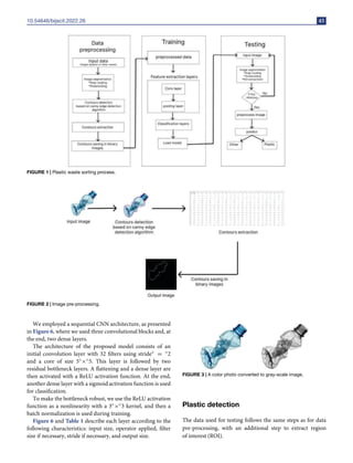
The creation of our system involved several distinct steps, as
illustrated in the schema in Figure 1. The process began by
feeding the model with the pre-processed dataset. The model
is then trained using the given dataset, where the parameters
of the CNN layers are updated. After the training phase,
the model moves on to the testing phase, where it predicts
whether the objects captured by the camera are plastics or
other types of waste.
Dataset pre-processing
In general, to process an image, you need to go through a pre-
processing stage where the image is cleaned. Pre-processing
consists of operations that the image must undergo. The
aim is to facilitate the use of the image in more complex
operations based on very precise image characteristics.
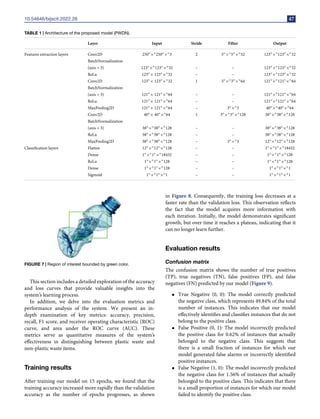
Our dataset has passed through some pre-processing
steps to achieve the best training results, as shown in
Figure 2.
Segmentation
A method of dividing a digital image into subgroups is called
image segmentation. This can reduce the complexity of the
image, making it easier to analyze.
Segmentation algorithms are used to group pixels in an
image. These groups are labeled to identify the objects that
make them up (5).
Gray-scale
Also known as black-and-white or monochrome image,
gray-scale image refers to an image or representation
that consists solely of shades of gray, ranging from pure
white to pure black.
Unlike color images, gray-scale images do not contain
any color information and only represent the brightness or
luminance values of the pixels, as shown in Figure 3. This
offers a simplified and focused representation of visual data,
allowing for specific analyses and ensuring accessibility in
various contexts (6).
Image thresholding
This is a technique used in image processing to convert a
gray-scale or color image into a binary image, as shown in
Figure 4.
The goal of thresholding is to separate objects or regions of
interest from the background based on their pixel intensities
to aid in image processing (7).
Contour detection
First of all, through a simple code, we extracted the contours
existing in each image of the dataset by following Canny
edge detection algorithm. Edge detection is a computational
technique that utilizes mathematical methods to identify
locations in an image where there are noticeable changes in
pixel intensity.
Canny is a filter that refers to a famous multi-step
algorithm to detect the edges of any input image, which was
developed by John F. Canny in 1986 (8).
The Canny edge detection algorithm is composed of the
following steps:
• Noise reduction: Apply a Gaussian blur to the image to
reduce noise and smooth out irregularities.
• Gradient calculation: Calculate the gradient magnitude
and orientation for each pixel in the blurred image.
• Non-maximum suppression: Suppress non-maximum
gradient values by thinning the edges to a single
pixel thickness.
• Thresholding: Apply thresholding to classify the
remaining pixels as either strong edges, weak edges, or
non-edges based on gradient magnitudes.
• Edge tracking by hysteresis: Connecting weak edges to
strong edges, thereby forming complete edge contours.
Weak edges that are not connected to any strong edges
are disregarded.
Following the application of Canny’s filter, we proceeded
to transform the detected contour points into a tabular
representation stored as a CSV (Comma-Separated Values)
file. Subsequently, the CSV file was further processed
to generate binary images through another simple code,
exclusively representing the shapes present in each image. As
a result, our dataset assumed the structure illustrated in the
aforementioned schema.
This representation can facilitate feature extraction, aid
in model interpretation, reduce dimensionality, and enhance
the training process for our model, as shown in Figure 5.
Plastic waste detection network (PWDN)
The Plastic Waste Detection Network (PWDN) is a CNN.
This is the core of our proposal.
10.54646/bijscit.2022.26 45
FIGURE 1 | Plastic waste sorting process.
FIGURE 2 | Image pre-processing.
We employed a sequential CNN architecture, as presented
in Figure 6, where we used three convolutional blocks and, at
the end, two dense layers.
The architecture of the proposed model consists of an
initial convolution layer with 32 filters using stride◦ = ◦2
and a core of size 5◦×◦5. This layer is followed by two
residual bottleneck layers. A flattening and a dense layer are
then activated with a ReLU activation function. At the end,
another dense layer with a sigmoid activation function is used
for classification.
To make the bottleneck robust, we use the ReLU activation
function as a nonlinearity with a 3◦×◦3 kernel, and then a
batch normalization is used during training.
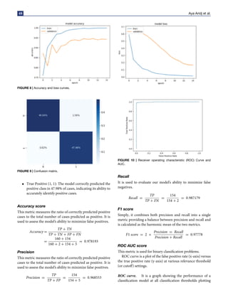
Figure 6 and Table 1 describe each layer according to the
following characteristics: input size, operator applied, filter
size if necessary, stride if necessary, and output size.
FIGURE 3 | A color photo converted to gray-scale image.
Plastic detection
The data used for testing follows the same steps as for data
pre-processing, with an additional step to extract region
of interest (ROI).
46 Aya Aridj et al.
FIGURE 4 | A gray-scale image after thresholding.
ROI refers to a specific area or region within an image
that is of particular interest for further analysis. In our
context, the ROI corresponds to the portion of the image
that potentially contains plastic waste objects, as shown in
Figure 7 (9).
After applying all the above algorithms, the images are
then standardized using test_datagenerator, which prepares
the images for prediction by applying the necessary
transformations and pre-processing.
FIGURE 5 | Canny edge detection.
The pre-trained model then applies its learned
parameters and architecture to analyze the images and
generate predictions.
Test and validation
The ability to accurately identify plastic waste items holds
great significance in combating environmental degradation.
FIGURE 6 | Proposed CNN model (PWDN).
10.54646/bijscit.2022.26 47
TABLE 1 | Architecture of the proposed model (PWDN).
Layer Input Stride Filter Output
Features extraction layers Conv2D 250◦×◦250◦×◦3 2 5◦×◦5◦×◦32 123◦×◦123◦×◦32
BatchNormalization
(axis = 3) 123◦×◦123◦×◦32 – – 123◦×◦123◦×◦32
ReLu 123◦× 123◦×◦32 – – 123◦×◦123◦×◦32
Conv2D 123◦× 123◦×◦32 1 3◦×◦3◦×◦64 121◦×◦121◦×◦64
BatchNormalization
(axis = 3) 121◦× 121◦×◦64 – – 121◦×◦121◦×◦64
ReLu 121◦× 121◦×◦64 – – 121◦×◦121◦×◦64
MaxPooling2D 121◦× 121◦×◦64 – 3◦×◦3 40◦×◦40◦×◦64
Conv2D 40◦× 40◦×◦64 1 3◦×◦3◦×◦128 38◦×◦38◦×◦128
BatchNormalization
(axis = 3) 38◦×◦38◦×◦128 – – 38◦×◦38◦×◦128
ReLu 38◦×◦38◦×◦128 – – 38◦×◦38◦×◦128
MaxPooling2D 38◦×◦38◦×◦128 – 3◦×◦3 12◦×◦12◦×◦128
Classification layers Flatten 12◦×◦12◦×◦128 – – 1◦×◦1◦×◦18432
Dense 1◦×◦1◦×◦18432 – – 1◦×◦1◦×◦128
ReLu 1◦×◦1◦×◦128 – – 1◦×◦1◦×◦128
Dense 1◦×◦1◦×◦128 – – 1◦×◦1◦×◦1
Sigmoid 1◦×◦1◦×◦1 – – 1◦×◦1◦×◦1
FIGURE 7 | Region of interest bounded by green color.
This section includes a detailed exploration of the accuracy
and loss curves that provide valuable insights into the
system’s learning process.
In addition, we delve into the evaluation metrics and
performance analysis of the system. We present an in-
depth examination of key metrics: accuracy, precision,
recall, F1 score, and receiver operating characteristic (ROC)
curve, and area under the ROC curve (AUC). These
metrics serve as quantitative measures of the system’s
effectiveness in distinguishing between plastic waste and
non-plastic waste items.
Training results
After training our model on 15 epochs, we found that the
training accuracy increased more rapidly than the validation
accuracy as the number of epochs progresses, as shown
in Figure 8. Consequently, the training loss decreases at a
faster rate than the validation loss. This observation reflects
the fact that the model acquires more information with
each iteration. Initially, the model demonstrates significant
growth, but over time it reaches a plateau, indicating that it
can no longer learn further.
Evaluation results
Confusion matrix
The confusion matrix shows the number of true positives
(TP), true negatives (TN), false positives (FP), and false
negatives (FN) predicted by our model (Figure 9).
• True Negative (0, 0): The model correctly predicted
the negative class, which represents 49.84% of the total
number of instances. This indicates that our model
effectively identifies and classifies instances that do not
belong to the positive class.
• False Positive (0, 1): The model incorrectly predicted
the positive class for 0.62% of instances that actually
belonged to the negative class. This suggests that
there is a small fraction of instances for which our
model generated false alarms or incorrectly identified
positive instances.
• False Negative (1, 0): The model incorrectly predicted
the negative class for 1.56% of instances that actually
belonged to the positive class. This indicates that there
is a small proportion of instances for which our model
failed to identify the positive class.
48 Aya Aridj et al.
FIGURE 8 | Accuracy and loss curves.
FIGURE 9 | Confusion matrix.
• True Positive (1, 1): The model correctly predicted the
positive class in 47.98% of cases, indicating its ability to
accurately identify positive cases.
Accuracy score
This metric measures the ratio of correctly predicted positive
cases to the total number of cases predicted as positive. It is
used to assess the model’s ability to minimize false positives.
Accuracy =
TP + TN
TP + TN + FP + FN
=
160 + 154
160 + 2 + 154 + 5
= 0.978193
Precision
This metric measures the ratio of correctly predicted positive
cases to the total number of cases predicted as positive. It is
used to assess the model’s ability to minimize false positives.
Precision =
TP
TP + FP
=
154
154 + 5
= 0.968553
FIGURE 10 | Receiver operating characteristic (ROC) Curve and
AUC.
Recall
It is used to evaluate our model’s ability to minimize false
negatives.
Recall =
TP
TP + FN
=
154
154 + 2
= 0.987179
F1 score
Simply, it combines both precision and recall into a single
metric providing a balance between precision and recall and
is calculated as the harmonic mean of the two metrics.
F1 score = 2 ×
Precision = Recall
Precision + Recall
= 0.97778
ROC AUC score
This metric is used for binary classification problems.
ROC curve is a plot of the false positive rate (x-axis) versus
the true positive rate (y-axis) at various relevance threshold
(or cutoff) settings.
ROC curve. It is a graph showing the performance of a
classification model at all classification thresholds plotting
10.54646/bijscit.2022.26 49
the true positive rate (recall) against the false positive
rate.
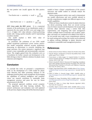
True Positive rate = sensitivity = recall =
TP
TP + FN
False Positive rate = 1 − specificity =
FP
FP + TN
AUC (Area under the ROC curve). It is a numerical
measure of the performance of our classification model. It
represents the area under the ROC curve and ranges from
0 to 1. A higher AUC value indicates a better-performing
model, with 1 being a perfect classifier and 0.5 representing
a random classifier.
Our model reached a ROC AUC value of
0.997669 (Figure 10).
In conclusion, the evaluation of our CNN model
yielded exceptional performance across various metrics.
Our model consistently achieved accurate predictions,
showcasing its effectiveness in correctly classifying the
target outcomes. Our system represents a significant step
toward a more sustainable and environmentally conscious
future. The insights gained from this evaluation serve as
a foundation for further research and development in the
field, driving us closer to effective solutions for plastic waste
reduction and mitigation.
Conclusion
To conclude this work, we presented a comprehensive
study on the development of a CNN model for plastic
waste detection that offers promising solutions to the
challenges posed by plastic waste management. By leveraging
the capabilities of artificial intelligence and computer
vision, our research contributes to sustainable waste
management practices and paves the way for future
advancements in the field.
The proposed approach combines several computer
vision algorithms and deep learning methods. The
system’s architecture and evaluation were well explained
in the previous chapters along with all the theoretical aspects
needed to foster a deeper comprehension of the system’s
intricacies and enable readers to critically analyze the
obtained results.
Various measurement metrics were used to demonstrate
our model’s effectiveness and were carefully selected to
provide comprehensive insights into different aspects of our
model’s capabilities.
While our binary classification system for plastic detection
has shown promising results, there are several exciting
areas for future research and development. By incorporating
real-time object detection using a camera feed, data
augmentation, and integrating with waste management
systems, multiple classes of materials, such as plastic, paper,
glass, and metal, are considered to be added in the future as
we can provide users with a more comprehensive solution
for waste sorting and recycling. Our system can be enhanced
to address evolving challenges in plastic detection and
contribute to sustainable waste management practices.
References
1. Ritchie H, Roser M. Plastic Pollution. Oxford: Our World in Data (2018).
2. Yang M, Thung G. Classification of Trash for Recyclability Status. CS229
project report. (Vol. 1). (2016).
3. Torres-Garcïa A, Rodea-Aragon O, Longoria-Gandara O, Sanchez-
Garcia F, Gonzalez-Jimenez LE. Intelligent waste separator. Computacion
Sistemas. (2015) 19:487–500.
4. Mittal G, Kaushal BY, Mohit G, Narayanan CK. Spotgarbage: smartphone
app to detect garbage using deep learning. Proceedings of the 2016 ACM
International Joint Conference on Pervasive and Ubiquitous Computing.
New York, NY: (2016). p. 940–5.
5. Datagen. Image Segmentation. (2023). Available online at: https://datagen.
tech/guides/image-annotation/image-segmentation/ (accessed July 02,
2023).
6. Fisher R, Perkins A. Grayscale Images. (2000). Available online at:
https://homepages.inf.ed.ac.uk/rbf/HIPR2/gryimage.htm (accessed July
02, 2023).
7. Geospatial LH. Image Thresholding. (2023). Available online at: https://
www.l3harrisgeospatial.com/docs/ImageThresholding.html (accessed
July 02, 2023)
8. Towards AI. What is a Canny Edge Detection Algorithm? (2023).
New York, NY: Towards AI.
9. SmartRay. Region of Interest (ROI). (2023). Available online at: https:
//www.smartray.com/glossary/region-of-interest-roi/ (accessed July 02,
2023).

CNN-based plastic waste detection system

  • 1.
    BOHR International Journalof Smart Computing and Information Technology 2022, Vol. 3, No. 1, pp. 43–49 DOI: 10.54646/bijscit.2022.26 www.bohrpub.com REVIEW CNN-based plastic waste detection system Grourou Aya Aridj1, Louchen Saher1 and Guezouli Larbi2* 1University of Batna 2, Batna, Algeria 2LEREESI, Higher National School of Renewable Energies, Environment and Sustainable Development, Batna, Algeria *Correspondence: Guezouli Larbi, larbi.guezouli@hns-re2sd.dz Received: 18 June 2022; Accepted: 08 July 2022; Published: 30 July 2022 Plastic waste has become a pressing global concern in recent decades, posing significant challenges to our environment due to its non-biodegradable nature and causing significant pollution and damage to our planet. Recycling plastic waste is one of the most effective solutions to this dilemma, which is why the aim of our project was to create a system that detects plastic waste using a large dataset with labeled data and one of the most famous deep learning neural networks, “Convolutional Neural Networks,” to classify and speed up the waste collection process and provide an easier recycling process. Thanks to our work, we have achieved 97% accuracy. Keywords: plastic waste detection, Convolutional Neural Networks (CNN), deep learning (DL), real-time, waste management Introduction Plastic waste is a major environmental problem. According to the latest statistics, the annual global production of plastic waste is over 300 million tons (1), and due to its non-biodegradable nature, plastic waste accumulates in landfills for hundreds of years, causing pollution, water contamination, and life-threatening problems for all creatures. The plastic recycling process can be a big help in reducing the harm caused by plastic waste. Several new technologies are being developed as well, such as pyrolysis, which can be used to convert plastic waste into oil and gas, and depolymerization, which can be used to break down plastic into its original components. To facilitate the implementation and realization of these technologies, we propose a system based on artificial intelligence that detects plastic waste using deep learning’s commonly used model the convolutional NeuralNetwork (CNN). The detection of waste requires precision and sharpness in many factors to obtain the best results. A comparison study was performed by Yang and Thung (2) to help with the recycling process using computer vision and predicting waste type only by vision. The reliance on hand-collected data in their project entitled “Classification of Trash for Recyclability Status” raises concerns about the dataset’s representativeness and potential biases. It is crucial to ensure that the dataset encompasses a diverse range of waste materials, considering that waste items can vary significantly in appearance, shape, and condition. It is worth exploring alternative feature extraction techniques and optimizing the CNN architecture to potentially enhance the models’ predictive capabilities. As seen in the Intelligent Waste Separator project (3), when K-Nearest Neighbor (KNN) and Health information management (HIM) methods were implemented, they relied on the points surrounding the shape of the object, which prevented the system from detecting deformed waste. This can be a major deficiency, hence the waste generally comes in multiple shapes and conditions. Arghadeep Mitra (4) stated that “The main issue of this project was the dataset which includes images that are slightly different from local waste materials,” which caused the model to predict some of the images wrongly. Therefore, using a collection of datasets collected from actual dirty, real places and images containing multiple objects in his 43
  • 2.
    44 Aya Aridjet al. training process might have boosted his model’s ability to predict better. The detection of waste demands attention to detail and precision across various factors. For example, the limitations faced in the previously shown works, underscore the importance of employing advanced techniques and comprehensive datasets to achieve better prediction results. The manuscript is organized as follows: After a general introduction, subsequent sections discuss the plastic waste sorting systems and validation of the proposed work. Finally, a general conclusion is given. Plastic waste sorting system The creation of our system involved several distinct steps, as illustrated in the schema in Figure 1. The process began by feeding the model with the pre-processed dataset. The model is then trained using the given dataset, where the parameters of the CNN layers are updated. After the training phase, the model moves on to the testing phase, where it predicts whether the objects captured by the camera are plastics or other types of waste. Dataset pre-processing In general, to process an image, you need to go through a pre- processing stage where the image is cleaned. Pre-processing consists of operations that the image must undergo. The aim is to facilitate the use of the image in more complex operations based on very precise image characteristics. Our dataset has passed through some pre-processing steps to achieve the best training results, as shown in Figure 2. Segmentation A method of dividing a digital image into subgroups is called image segmentation. This can reduce the complexity of the image, making it easier to analyze. Segmentation algorithms are used to group pixels in an image. These groups are labeled to identify the objects that make them up (5). Gray-scale Also known as black-and-white or monochrome image, gray-scale image refers to an image or representation that consists solely of shades of gray, ranging from pure white to pure black. Unlike color images, gray-scale images do not contain any color information and only represent the brightness or luminance values of the pixels, as shown in Figure 3. This offers a simplified and focused representation of visual data, allowing for specific analyses and ensuring accessibility in various contexts (6). Image thresholding This is a technique used in image processing to convert a gray-scale or color image into a binary image, as shown in Figure 4. The goal of thresholding is to separate objects or regions of interest from the background based on their pixel intensities to aid in image processing (7). Contour detection First of all, through a simple code, we extracted the contours existing in each image of the dataset by following Canny edge detection algorithm. Edge detection is a computational technique that utilizes mathematical methods to identify locations in an image where there are noticeable changes in pixel intensity. Canny is a filter that refers to a famous multi-step algorithm to detect the edges of any input image, which was developed by John F. Canny in 1986 (8). The Canny edge detection algorithm is composed of the following steps: • Noise reduction: Apply a Gaussian blur to the image to reduce noise and smooth out irregularities. • Gradient calculation: Calculate the gradient magnitude and orientation for each pixel in the blurred image. • Non-maximum suppression: Suppress non-maximum gradient values by thinning the edges to a single pixel thickness. • Thresholding: Apply thresholding to classify the remaining pixels as either strong edges, weak edges, or non-edges based on gradient magnitudes. • Edge tracking by hysteresis: Connecting weak edges to strong edges, thereby forming complete edge contours. Weak edges that are not connected to any strong edges are disregarded. Following the application of Canny’s filter, we proceeded to transform the detected contour points into a tabular representation stored as a CSV (Comma-Separated Values) file. Subsequently, the CSV file was further processed to generate binary images through another simple code, exclusively representing the shapes present in each image. As a result, our dataset assumed the structure illustrated in the aforementioned schema. This representation can facilitate feature extraction, aid in model interpretation, reduce dimensionality, and enhance the training process for our model, as shown in Figure 5. Plastic waste detection network (PWDN) The Plastic Waste Detection Network (PWDN) is a CNN. This is the core of our proposal.
  • 3.
    10.54646/bijscit.2022.26 45 FIGURE 1| Plastic waste sorting process. FIGURE 2 | Image pre-processing. We employed a sequential CNN architecture, as presented in Figure 6, where we used three convolutional blocks and, at the end, two dense layers. The architecture of the proposed model consists of an initial convolution layer with 32 filters using stride◦ = ◦2 and a core of size 5◦×◦5. This layer is followed by two residual bottleneck layers. A flattening and a dense layer are then activated with a ReLU activation function. At the end, another dense layer with a sigmoid activation function is used for classification. To make the bottleneck robust, we use the ReLU activation function as a nonlinearity with a 3◦×◦3 kernel, and then a batch normalization is used during training. Figure 6 and Table 1 describe each layer according to the following characteristics: input size, operator applied, filter size if necessary, stride if necessary, and output size. FIGURE 3 | A color photo converted to gray-scale image. Plastic detection The data used for testing follows the same steps as for data pre-processing, with an additional step to extract region of interest (ROI).
  • 4.
    46 Aya Aridjet al. FIGURE 4 | A gray-scale image after thresholding. ROI refers to a specific area or region within an image that is of particular interest for further analysis. In our context, the ROI corresponds to the portion of the image that potentially contains plastic waste objects, as shown in Figure 7 (9). After applying all the above algorithms, the images are then standardized using test_datagenerator, which prepares the images for prediction by applying the necessary transformations and pre-processing. FIGURE 5 | Canny edge detection. The pre-trained model then applies its learned parameters and architecture to analyze the images and generate predictions. Test and validation The ability to accurately identify plastic waste items holds great significance in combating environmental degradation. FIGURE 6 | Proposed CNN model (PWDN).
  • 5.
    10.54646/bijscit.2022.26 47 TABLE 1| Architecture of the proposed model (PWDN). Layer Input Stride Filter Output Features extraction layers Conv2D 250◦×◦250◦×◦3 2 5◦×◦5◦×◦32 123◦×◦123◦×◦32 BatchNormalization (axis = 3) 123◦×◦123◦×◦32 – – 123◦×◦123◦×◦32 ReLu 123◦× 123◦×◦32 – – 123◦×◦123◦×◦32 Conv2D 123◦× 123◦×◦32 1 3◦×◦3◦×◦64 121◦×◦121◦×◦64 BatchNormalization (axis = 3) 121◦× 121◦×◦64 – – 121◦×◦121◦×◦64 ReLu 121◦× 121◦×◦64 – – 121◦×◦121◦×◦64 MaxPooling2D 121◦× 121◦×◦64 – 3◦×◦3 40◦×◦40◦×◦64 Conv2D 40◦× 40◦×◦64 1 3◦×◦3◦×◦128 38◦×◦38◦×◦128 BatchNormalization (axis = 3) 38◦×◦38◦×◦128 – – 38◦×◦38◦×◦128 ReLu 38◦×◦38◦×◦128 – – 38◦×◦38◦×◦128 MaxPooling2D 38◦×◦38◦×◦128 – 3◦×◦3 12◦×◦12◦×◦128 Classification layers Flatten 12◦×◦12◦×◦128 – – 1◦×◦1◦×◦18432 Dense 1◦×◦1◦×◦18432 – – 1◦×◦1◦×◦128 ReLu 1◦×◦1◦×◦128 – – 1◦×◦1◦×◦128 Dense 1◦×◦1◦×◦128 – – 1◦×◦1◦×◦1 Sigmoid 1◦×◦1◦×◦1 – – 1◦×◦1◦×◦1 FIGURE 7 | Region of interest bounded by green color. This section includes a detailed exploration of the accuracy and loss curves that provide valuable insights into the system’s learning process. In addition, we delve into the evaluation metrics and performance analysis of the system. We present an in- depth examination of key metrics: accuracy, precision, recall, F1 score, and receiver operating characteristic (ROC) curve, and area under the ROC curve (AUC). These metrics serve as quantitative measures of the system’s effectiveness in distinguishing between plastic waste and non-plastic waste items. Training results After training our model on 15 epochs, we found that the training accuracy increased more rapidly than the validation accuracy as the number of epochs progresses, as shown in Figure 8. Consequently, the training loss decreases at a faster rate than the validation loss. This observation reflects the fact that the model acquires more information with each iteration. Initially, the model demonstrates significant growth, but over time it reaches a plateau, indicating that it can no longer learn further. Evaluation results Confusion matrix The confusion matrix shows the number of true positives (TP), true negatives (TN), false positives (FP), and false negatives (FN) predicted by our model (Figure 9). • True Negative (0, 0): The model correctly predicted the negative class, which represents 49.84% of the total number of instances. This indicates that our model effectively identifies and classifies instances that do not belong to the positive class. • False Positive (0, 1): The model incorrectly predicted the positive class for 0.62% of instances that actually belonged to the negative class. This suggests that there is a small fraction of instances for which our model generated false alarms or incorrectly identified positive instances. • False Negative (1, 0): The model incorrectly predicted the negative class for 1.56% of instances that actually belonged to the positive class. This indicates that there is a small proportion of instances for which our model failed to identify the positive class.
  • 6.
    48 Aya Aridjet al. FIGURE 8 | Accuracy and loss curves. FIGURE 9 | Confusion matrix. • True Positive (1, 1): The model correctly predicted the positive class in 47.98% of cases, indicating its ability to accurately identify positive cases. Accuracy score This metric measures the ratio of correctly predicted positive cases to the total number of cases predicted as positive. It is used to assess the model’s ability to minimize false positives. Accuracy = TP + TN TP + TN + FP + FN = 160 + 154 160 + 2 + 154 + 5 = 0.978193 Precision This metric measures the ratio of correctly predicted positive cases to the total number of cases predicted as positive. It is used to assess the model’s ability to minimize false positives. Precision = TP TP + FP = 154 154 + 5 = 0.968553 FIGURE 10 | Receiver operating characteristic (ROC) Curve and AUC. Recall It is used to evaluate our model’s ability to minimize false negatives. Recall = TP TP + FN = 154 154 + 2 = 0.987179 F1 score Simply, it combines both precision and recall into a single metric providing a balance between precision and recall and is calculated as the harmonic mean of the two metrics. F1 score = 2 × Precision = Recall Precision + Recall = 0.97778 ROC AUC score This metric is used for binary classification problems. ROC curve is a plot of the false positive rate (x-axis) versus the true positive rate (y-axis) at various relevance threshold (or cutoff) settings. ROC curve. It is a graph showing the performance of a classification model at all classification thresholds plotting
  • 7.
    10.54646/bijscit.2022.26 49 the truepositive rate (recall) against the false positive rate. True Positive rate = sensitivity = recall = TP TP + FN False Positive rate = 1 − specificity = FP FP + TN AUC (Area under the ROC curve). It is a numerical measure of the performance of our classification model. It represents the area under the ROC curve and ranges from 0 to 1. A higher AUC value indicates a better-performing model, with 1 being a perfect classifier and 0.5 representing a random classifier. Our model reached a ROC AUC value of 0.997669 (Figure 10). In conclusion, the evaluation of our CNN model yielded exceptional performance across various metrics. Our model consistently achieved accurate predictions, showcasing its effectiveness in correctly classifying the target outcomes. Our system represents a significant step toward a more sustainable and environmentally conscious future. The insights gained from this evaluation serve as a foundation for further research and development in the field, driving us closer to effective solutions for plastic waste reduction and mitigation. Conclusion To conclude this work, we presented a comprehensive study on the development of a CNN model for plastic waste detection that offers promising solutions to the challenges posed by plastic waste management. By leveraging the capabilities of artificial intelligence and computer vision, our research contributes to sustainable waste management practices and paves the way for future advancements in the field. The proposed approach combines several computer vision algorithms and deep learning methods. The system’s architecture and evaluation were well explained in the previous chapters along with all the theoretical aspects needed to foster a deeper comprehension of the system’s intricacies and enable readers to critically analyze the obtained results. Various measurement metrics were used to demonstrate our model’s effectiveness and were carefully selected to provide comprehensive insights into different aspects of our model’s capabilities. While our binary classification system for plastic detection has shown promising results, there are several exciting areas for future research and development. By incorporating real-time object detection using a camera feed, data augmentation, and integrating with waste management systems, multiple classes of materials, such as plastic, paper, glass, and metal, are considered to be added in the future as we can provide users with a more comprehensive solution for waste sorting and recycling. Our system can be enhanced to address evolving challenges in plastic detection and contribute to sustainable waste management practices. References 1. Ritchie H, Roser M. Plastic Pollution. Oxford: Our World in Data (2018). 2. Yang M, Thung G. Classification of Trash for Recyclability Status. CS229 project report. (Vol. 1). (2016). 3. Torres-Garcïa A, Rodea-Aragon O, Longoria-Gandara O, Sanchez- Garcia F, Gonzalez-Jimenez LE. Intelligent waste separator. Computacion Sistemas. (2015) 19:487–500. 4. Mittal G, Kaushal BY, Mohit G, Narayanan CK. Spotgarbage: smartphone app to detect garbage using deep learning. Proceedings of the 2016 ACM International Joint Conference on Pervasive and Ubiquitous Computing. New York, NY: (2016). p. 940–5. 5. Datagen. Image Segmentation. (2023). Available online at: https://datagen. tech/guides/image-annotation/image-segmentation/ (accessed July 02, 2023). 6. Fisher R, Perkins A. Grayscale Images. (2000). Available online at: https://homepages.inf.ed.ac.uk/rbf/HIPR2/gryimage.htm (accessed July 02, 2023). 7. Geospatial LH. Image Thresholding. (2023). Available online at: https:// www.l3harrisgeospatial.com/docs/ImageThresholding.html (accessed July 02, 2023) 8. Towards AI. What is a Canny Edge Detection Algorithm? (2023). New York, NY: Towards AI. 9. SmartRay. Region of Interest (ROI). (2023). Available online at: https: //www.smartray.com/glossary/region-of-interest-roi/ (accessed July 02, 2023).