Circuitikzmanual

CircuiTikZ
version 0.6 (2016/06/06)
Massimo A. Redaelli (m.redaelli@gmail.com)
Stefan Lindner (stefan.lindner@fau.de)
Stefan Erhardt (stefan.erhardt@fau.de)
June 6, 2016
Contents
1 Introduction 1
1.1 About . . . . . . . . . . . . . . . . . . . . . . . . . . . . . . . . . . . . . . . . . . . 1
1.2 Loading the package . . . . . . . . . . . . . . . . . . . . . . . . . . . . . . . . . . . 1
1.3 Requirements . . . . . . . . . . . . . . . . . . . . . . . . . . . . . . . . . . . . . . . 1
1.4 Incompatible packages . . . . . . . . . . . . . . . . . . . . . . . . . . . . . . . . . . 2
1.5 License . . . . . . . . . . . . . . . . . . . . . . . . . . . . . . . . . . . . . . . . . . . 2
1.6 Feedback . . . . . . . . . . . . . . . . . . . . . . . . . . . . . . . . . . . . . . . . . 2
2 Incompabilities between version 2
3 Package options 2
4 The components 4
4.1 Monopoles . . . . . . . . . . . . . . . . . . . . . . . . . . . . . . . . . . . . . . . . . 5
4.2 Bipoles . . . . . . . . . . . . . . . . . . . . . . . . . . . . . . . . . . . . . . . . . . . 7
4.2.1 Instruments . . . . . . . . . . . . . . . . . . . . . . . . . . . . . . . . . . . . 7
4.2.2 Basic resistive bipoles . . . . . . . . . . . . . . . . . . . . . . . . . . . . . . 7
4.2.3 Resistors and the like . . . . . . . . . . . . . . . . . . . . . . . . . . . . . . 8
4.2.4 Diodes and such . . . . . . . . . . . . . . . . . . . . . . . . . . . . . . . . . 9
4.2.5 Other tripole-like diodes . . . . . . . . . . . . . . . . . . . . . . . . . . . . . 12
4.2.6 Basic dynamical bipoles . . . . . . . . . . . . . . . . . . . . . . . . . . . . . 13
4.2.7 Stationary sources . . . . . . . . . . . . . . . . . . . . . . . . . . . . . . . . 15
4.2.8 Sinusoidal sources . . . . . . . . . . . . . . . . . . . . . . . . . . . . . . . . 15
4.2.9 Special sources . . . . . . . . . . . . . . . . . . . . . . . . . . . . . . . . . . 16
4.2.10 DC sources . . . . . . . . . . . . . . . . . . . . . . . . . . . . . . . . . . . . 16
4.2.11 Mechanical Analogy . . . . . . . . . . . . . . . . . . . . . . . . . . . . . . . 16
4.2.12 Switch . . . . . . . . . . . . . . . . . . . . . . . . . . . . . . . . . . . . . . . 17
4.2.13 Block diagram components . . . . . . . . . . . . . . . . . . . . . . . . . . . 17
4.3 Tripoles . . . . . . . . . . . . . . . . . . . . . . . . . . . . . . . . . . . . . . . . . . 19
4.3.1 Controlled sources . . . . . . . . . . . . . . . . . . . . . . . . . . . . . . . . 19
4.3.2 Transistors . . . . . . . . . . . . . . . . . . . . . . . . . . . . . . . . . . . . 20
4.3.3 Block diagram . . . . . . . . . . . . . . . . . . . . . . . . . . . . . . . . . . 24
4.3.4 Switch . . . . . . . . . . . . . . . . . . . . . . . . . . . . . . . . . . . . . . . 25
4.3.5 Electro-Mechanical Devices . . . . . . . . . . . . . . . . . . . . . . . . . . . 25
4.4 Double bipoles . . . . . . . . . . . . . . . . . . . . . . . . . . . . . . . . . . . . . . 26
4.5 Logic gates . . . . . . . . . . . . . . . . . . . . . . . . . . . . . . . . . . . . . . . . 27
1

4.6 Amplifiers . . . . . . . . . . . . . . . . . . . . . . . . . . . . . . . . . . . . . . . . . 29
4.7 Support shapes . . . . . . . . . . . . . . . . . . . . . . . . . . . . . . . . . . . . . . 30
5 Usage 30
5.1 Labels . . . . . . . . . . . . . . . . . . . . . . . . . . . . . . . . . . . . . . . . . . . 31
5.2 Currents . . . . . . . . . . . . . . . . . . . . . . . . . . . . . . . . . . . . . . . . . . 32
5.3 Voltages . . . . . . . . . . . . . . . . . . . . . . . . . . . . . . . . . . . . . . . . . . 33
5.3.1 European style . . . . . . . . . . . . . . . . . . . . . . . . . . . . . . . . . . 33
5.3.2 American style . . . . . . . . . . . . . . . . . . . . . . . . . . . . . . . . . . 34
5.4 Nodes . . . . . . . . . . . . . . . . . . . . . . . . . . . . . . . . . . . . . . . . . . . 35
5.5 Special components . . . . . . . . . . . . . . . . . . . . . . . . . . . . . . . . . . . . 36
5.6 Integration with siunitx . . . . . . . . . . . . . . . . . . . . . . . . . . . . . . . . 37
5.7 Mirroring . . . . . . . . . . . . . . . . . . . . . . . . . . . . . . . . . . . . . . . . . 38
5.8 Putting them together . . . . . . . . . . . . . . . . . . . . . . . . . . . . . . . . . . 38
6 Not only bipoles 39
6.1 Anchors . . . . . . . . . . . . . . . . . . . . . . . . . . . . . . . . . . . . . . . . . . 39
6.1.1 Logical ports . . . . . . . . . . . . . . . . . . . . . . . . . . . . . . . . . . . 39
6.1.2 Transistors . . . . . . . . . . . . . . . . . . . . . . . . . . . . . . . . . . . . 40
6.1.3 Other tripoles . . . . . . . . . . . . . . . . . . . . . . . . . . . . . . . . . . . 41
6.1.4 Operational amplifier . . . . . . . . . . . . . . . . . . . . . . . . . . . . . . 42
6.1.5 Double bipoles . . . . . . . . . . . . . . . . . . . . . . . . . . . . . . . . . . 43
6.2 Input arrows . . . . . . . . . . . . . . . . . . . . . . . . . . . . . . . . . . . . . . . 44
6.3 Labels and custom twoport boxes . . . . . . . . . . . . . . . . . . . . . . . . . . . . 44
6.4 Box option . . . . . . . . . . . . . . . . . . . . . . . . . . . . . . . . . . . . . . . . 44
6.5 Dash optional parts . . . . . . . . . . . . . . . . . . . . . . . . . . . . . . . . . . . 45
6.6 Transistor paths . . . . . . . . . . . . . . . . . . . . . . . . . . . . . . . . . . . . . 45
7 Customization 46
7.1 Parameters . . . . . . . . . . . . . . . . . . . . . . . . . . . . . . . . . . . . . . . . 46
7.2 Components size . . . . . . . . . . . . . . . . . . . . . . . . . . . . . . . . . . . . . 47
7.3 Colors . . . . . . . . . . . . . . . . . . . . . . . . . . . . . . . . . . . . . . . . . . . 48
8 FAQ 49
9 Examples 50
10 Changelog 55
Index of the components 58
1 Introduction
1.1 About
CircuiTikZ was initiated by Massimo Redaelli in 2007, who was working as a research assistant
at the Polytechnic University of Milan, Italy, and needed a tool for creating exercises and exams.
After he left University in 2010 the development of CircuiTikZ slowed down, since LATEX is mainly
established in the academic world. In 2015 Stefan Lindner and Stefan Erhardt, both working as
research assistants at the University of Erlangen-Nürnberg, Germany, joined the team and now
maintain the project together with the initial author.
The use of CircuiTikZ is, of course, not limited to academic teaching. The package gets widely
used by engineers for typesetting electronic circuits for articles and publications all over the world.
2

This documentation is somewhat scant. Hopefully the authors will find the leisure to improve
it some day.
1.2 Loading the package
LATEX ConTEXt1
usepackage{circuitikz} usemodule[circuitikz]
TikZ will be automatically loaded.
CircuiTikZ commands are just TikZ commands, so a minimum usage example would be:
R1
1 tikz draw (0,0) to[R=$R_1$] (2,0);
1.3 Requirements
• tikz, version ≥ 2;
• xstring, not older than 2009/03/13;
• siunitx, if using siunitx option.
1.4 Incompatible packages
TikZ’s own circuit library, which is based on CircuiTikZ, (re?)defines several styles used by this
library. In order to have them work together you can use the compatibility package option,
which basically prefixes the names of all CircuiTikZ to[] styles with an asterisk.
So, if loaded with said option, one must write (0,0) to[*R] (2,0) and, for transistors on a
path, (0,0) to[*Tnmos] (2,0), and so on (but (0,0) node[nmos] {}). See example at page 55.
1.5 License
Copyright © 2007–2016 Massimo Redaelli. This package is author-maintained. Permission is
granted to copy, distribute and/or modify this software under the terms of the LATEX Project
Public License, version 1.3.1, or the GNU Public License. This software is provided ‘as is’, without
warranty of any kind, either expressed or implied, including, but not limited to, the implied
warranties of merchantability and fitness for a particular purpose.
1.6 Feedback
The easiest way to contact the authors is via the official Github repository: https://github.com/
circuitikz/circuitikz/issues
2 Incompabilities between version
Here, we will provide a list of incompabilitys between different version of circuitikz. We will try
to hold this list short, but sometimes it is easier to break with old syntax than including a lot of
switches and compatibility layers.
• Since v0.5.1: The parts pfet,pigfete,pigfetebulk and pigfetd are now mirrored by default.
Please adjust your yscale-option to correct this.
• Since v0.5: New voltage counting direction, here exists an option to use the old behaviour
1ConTEXt suppurt was added mostly thanks to Mojca Miklavec and Aditya Mahajan.
3

3 Package options
Circuit people are very opinionated about their symbols. In order to meet the individual gusto you
can set a bunch of package options. The standard options are what the authors like, for example
you get this:
2 Ω
84 V
?
84 V
1 begin{circuitikz}
2 draw (0,0) to[R=2<ohm>, i=?, v=84<volt>] (2,0) --
3 (2,2) to[V<=84<volt>] (0,2)
4 -- (0,0);
5 end{circuitikz}
Feel free to load the package with your own cultural options:
LATEX ConTEXt
usepackage[american]{circuitikz} usemodule[circuitikz][american]
2 Ω
+ −
84 V
?
+
−
84 V
1 begin{circuitikz}
2 draw (0,0) to[R=2<ohm>, i=?, v=84<volt>] (2,0) --
3 (2,2) to[V<=84<volt>] (0,2)
4 -- (0,0);
5 end{circuitikz}
Here is the list of all the options:
• europeanvoltages: uses arrows to define voltages, and uses european-style voltage sources;
• americanvoltages: uses − and + to define voltages, and uses american-style voltage sources;
• europeancurrents: uses european-style current sources;
• americancurrents: uses american-style current sources;
• europeanresistors: uses rectangular empty shape for resistors, as per european standards;
• americanresistors: uses zig-zag shape for resistors, as per american standards;
• europeaninductors: uses rectangular filled shape for inductors, as per european standards;
• americaninductors: uses ”4-bumps” shape for inductors, as per american standards;
• cuteinductors: uses my personal favorite, ”pig-tailed” shape for inductors;
• americanports: uses triangular logic ports, as per american standards;
• europeanports: uses rectangular logic ports, as per european standards;
• americangfsurgearrester: uses round gas filled surge arresters, as per american standards;
• europeangfsurgearrester: uses rectangular gas filled surge arresters, as per european
standards;
• european: equivalent to europeancurrents, europeanvoltages, europeanresistors, europeaninductors,
europeanports, europeangfsurgearrester;
4

• american: equivalent to americancurrents, americanvoltages, americanresistors, americaninductors,
americanports, americangfsurgearrester;
• siunitx: integrates with SIunitx package. If labels, currents or voltages are of the form
#1<#2> then what is shown is actually SI{#1}{#2};
• nosiunitx: labels are not interpreted as above;
• fulldiode: the various diodes are drawn and filled by default, i.e. when using styles such
as diode, D, sD, …Other diode styles can always be forced with e.g. Do, D-, …
• strokediode: the various diodes are drawn and stroke by default, i.e. when using styles
such as diode, D, sD, …Other diode styles can always be forced with e.g. Do, D*, …
• emptydiode: the various diodes are drawn but not filled by default, i.e. when using styles
such as D, sD, …Other diode styles can always be forced with e.g. Do, D-, …
• arrowmos: pmos and nmos have arrows analogous to those of pnp and npn transistors;
• noarrowmos: pmos and nmos do not have arrows analogous to those of pnp and npn tran-
sistors;
• fetbodydiode: draw the body diode of a FET;
• nofetbodydiode: do not draw the body diode of a FET;
• fetsolderdot: draw solderdot at bulk-source junction of some transistors;
• nofetsolderdot: do not draw solderdot at bulk-source junction of some transistors;
• emptypmoscircle: the circle at the gate of a pmos transistor gets not filled;
• lazymos: draws lazy nmos and pmos transistors. Chip designers with huge circuits prefer
this notation;
• straightlabels: labels on bipoles are always printed straight up, i.e. with horizontal base-
line;
• rotatelabels: labels on bipoles are always printed aligned along the bipole;
• smartlabels: labels on bipoles are rotated along the bipoles, unless the rotation is very
close to multiples of 90°;
• compatibility: makes it possibile to load CircuiTikZ and TikZ circuit library together.
• oldvoltagedirection: Use old(erronous) way of voltage direction having a difference be-
tween european and american direction
• betterproportions2
: nicer proportions of transistors in comparision to resistors;
The old options in the singular (like american voltage) are still available for compatibility,
but are discouraged.
Loading the package with no options is equivalent to my own personal liking, that is to the
following options:
[nofetsolderdot,nooldvoltagedirection,europeancurrents,europeanvoltages,americanports,americanres
In ConTEXt the options are similarly specified: current=european|american, voltage=european|american,
resistor=american|european, inductor=cute|american|european, logic=american|european,
siunitx=true|false, arrowmos=false|true.
2May change in the future!
5

4 The components
Here follows the list of all the shapes defined by CircuiTikZ. These are all pgf nodes, so they are
usable in both pgf and TikZ.
Drawing normal components
Normal components (monopoles, multipoles) can be drawn at a specified point with this syntax,
where #1 is the name of the component:
begin{center}begin{circuitikz} draw
(0,0) node[#1,#2] (#3) {#4}
; end{circuitikz} end{center}
Explanation of the parameters:
#1: component name3
(mandatory)
#2: list of comma separated options (optional)
#3: name of an anchor (optional)
#4: text written to the text anchor of the component (optional)
Note for TikZ newbies: Nodes must have curly brackets at the end, even when empty.
An optional anchor (#3) can be defined within round brackets to be addressed again later on.
And please don’t forget the semicolon to terminate the draw command.
Drawing bipoles/two-ports
Bipoles/Two-ports (plus some special components) can be drawn between two points using the
following command:
begin{center}begin{circuitikz} draw
(0,0) to[#1,#2] (2,0)
; end{circuitikz} end{center}
Explanation of the parameters:
#1: component name (mandatory)
#2: list of comma separated options (optional)
Transistors and some other components can also be placed using the syntax for bipoles. See
section 6.6.
If using the tikzexternalize feature, as of Tikz 2.1 all pictures must end with
end{tikzpicture}. Thus you cannot use the circuitikz environment.
Which is ok: just use the environment tikzpicture: everything will work there just fine.
4.1 Monopoles
• Ground (node[ground]{})
• Reference ground (node[rground]{})
3For using bipoles as nodes, the name of the node is #1shape.
6

• Signal ground (node[sground]{})
• Thicker ground (node[tground]{})
• Noiseless ground (node[nground]{})
• Protective ground (node[pground]{})
• Chassis ground4
(node[cground]{})
• Antenna (node[antenna]{})
• Receiving antenna (node[rxantenna]{})
• Transmitting antenna (node[txantenna]{})
4These last three were contributed by Luigi «Liverpool»)
7

• Transmission line stub (node[tlinestub]{})
• VCC/VDD (node[vcc]{})
• VEE/VSS (node[vee]{})
• match (node[match]{})
4.2 Bipoles
4.2.1 Instruments
• Ammeter (ammeter)
A
• Voltmeter (voltmeter)
V
• Ohmmeter (ohmmeter)
Ω
4.2.2 Basic resistive bipoles
• Short circuit (short)
• Open circuit (open)
• Lamp (lamp)
8

• Generic (symmetric) bipole (generic)
• Tunable generic bipole (tgeneric)
• Generic asymmetric bipole (ageneric)
• Generic asymmetric bipole (full) (fullgeneric)
• Tunable generic bipole (full) (tfullgeneric)
• Memristor (memristor, or Mr)
4.2.3 Resistors and the like
If (default behaviour) americanresistors option is active (or the style [american resistors]
is used), the resistor is displayed as follows:
• Resistor (R, or american resistor)
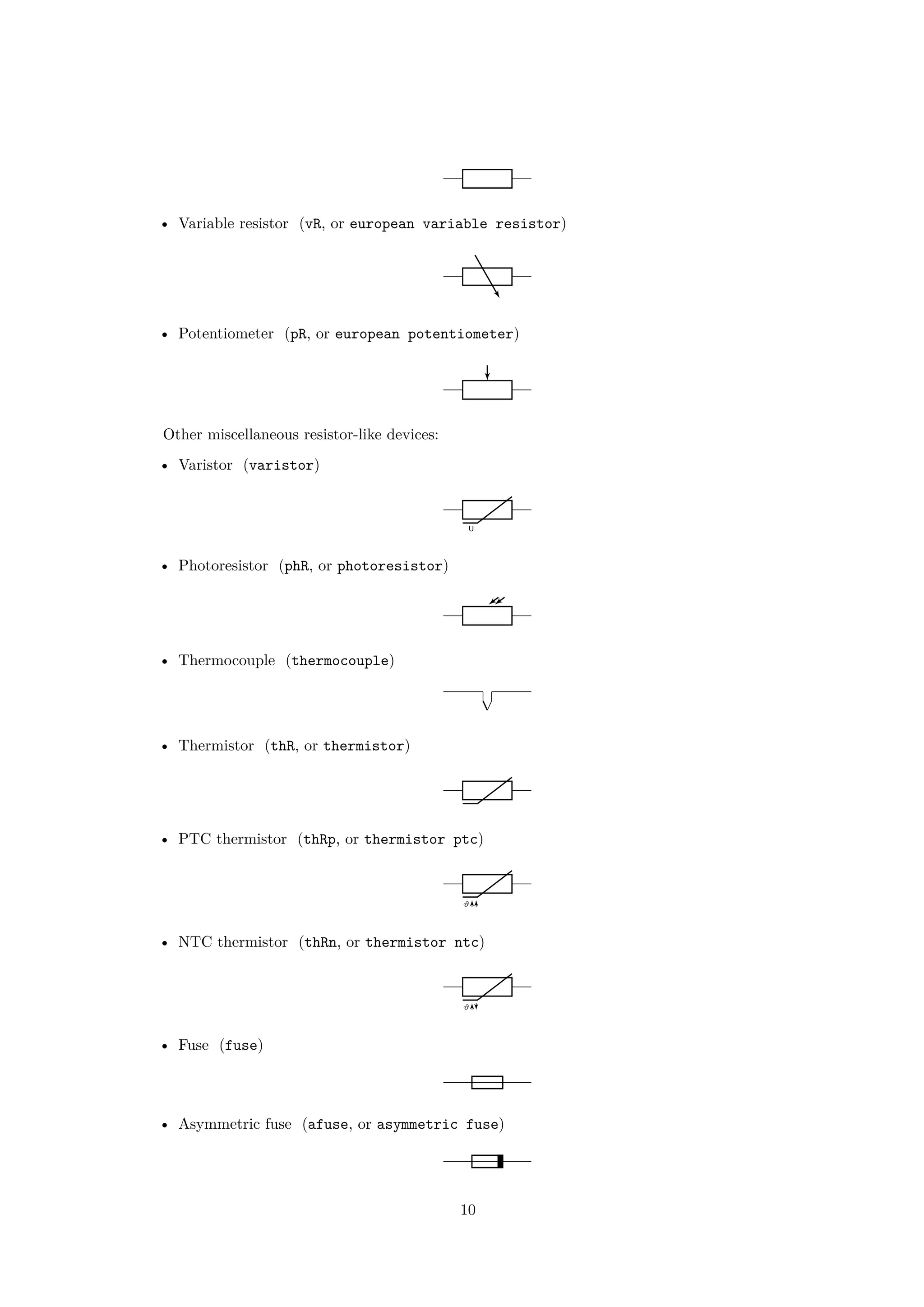
• Variable resistor (vR, or variable american resistor)
• Potentiometer (pR, or american potentiometer)
If instead europeanresistors option is active (or the style [european resistors] is used),
the resistors, variable resistors and potentiometers are displayed as follows:
• Resistor (R, or european resistor)
9

• Variable resistor (vR, or european variable resistor)
• Potentiometer (pR, or european potentiometer)
Other miscellaneous resistor-like devices:
• Varistor (varistor)
U
• Photoresistor (phR, or photoresistor)
• Thermocouple (thermocouple)
• Thermistor (thR, or thermistor)
• PTC thermistor (thRp, or thermistor ptc)
ϑ
• NTC thermistor (thRn, or thermistor ntc)
ϑ
• Fuse (fuse)
• Asymmetric fuse (afuse, or asymmetric fuse)
10

4.2.4 Diodes and such
• Empty diode (empty diode, or Do)
• Empty Schottky diode (empty Schottky diode, or sDo)
• Empty Zener diode (empty Zener diode, or zDo)
• Empty ZZener diode (empty ZZener diode, or zzDo)
• Empty tunnel diode (empty tunnel diode, or tDo)
• Empty photodiode (empty photodiode, or pDo)
• Empty led (empty led, or leDo)
• Empty varcap (empty varcap, or VCo)
• Full diode (full diode, or D*)
• Full Schottky diode (full Schottky diode, or sD*)
11

• Full Zener diode (full Zener diode, or zD*)
• Full ZZener diode (full ZZener diode, or zzD*)
• Full tunnel diode (full tunnel diode, or tD*)
• Full photodiode (full photodiode, or pD*)
• Full led (full led, or leD*)
• Full varcap (full varcap, or VC*)
• Stroke diode (stroke diode, or D-)
• Stroke Schottky diode (stroke Schottky diode, or sD-)
• Stroke Zener diode (stroke Zener diode, or zD-)
• Stroke ZZener diode (stroke ZZener diode, or zzD-)
12

• Stroke tunnel diode (stroke tunnel diode, or tD-)
• Stroke photodiode (stroke photodiode, or pD-)
• Stroke led (stroke led, or leD-)
• Stroke varcap (stroke varcap, or VC-)
4.2.5 Other tripole-like diodes
The following tripoles are entered with the usual command of the form
• Standard triac (shape depends on package option) (triac, or Tr)
• Empty triac (empty triac, or Tro)
• Full triac (full triac, or Tr*)
• Standard thyristor (shape depends on package option) (thyristor, or Ty)
13

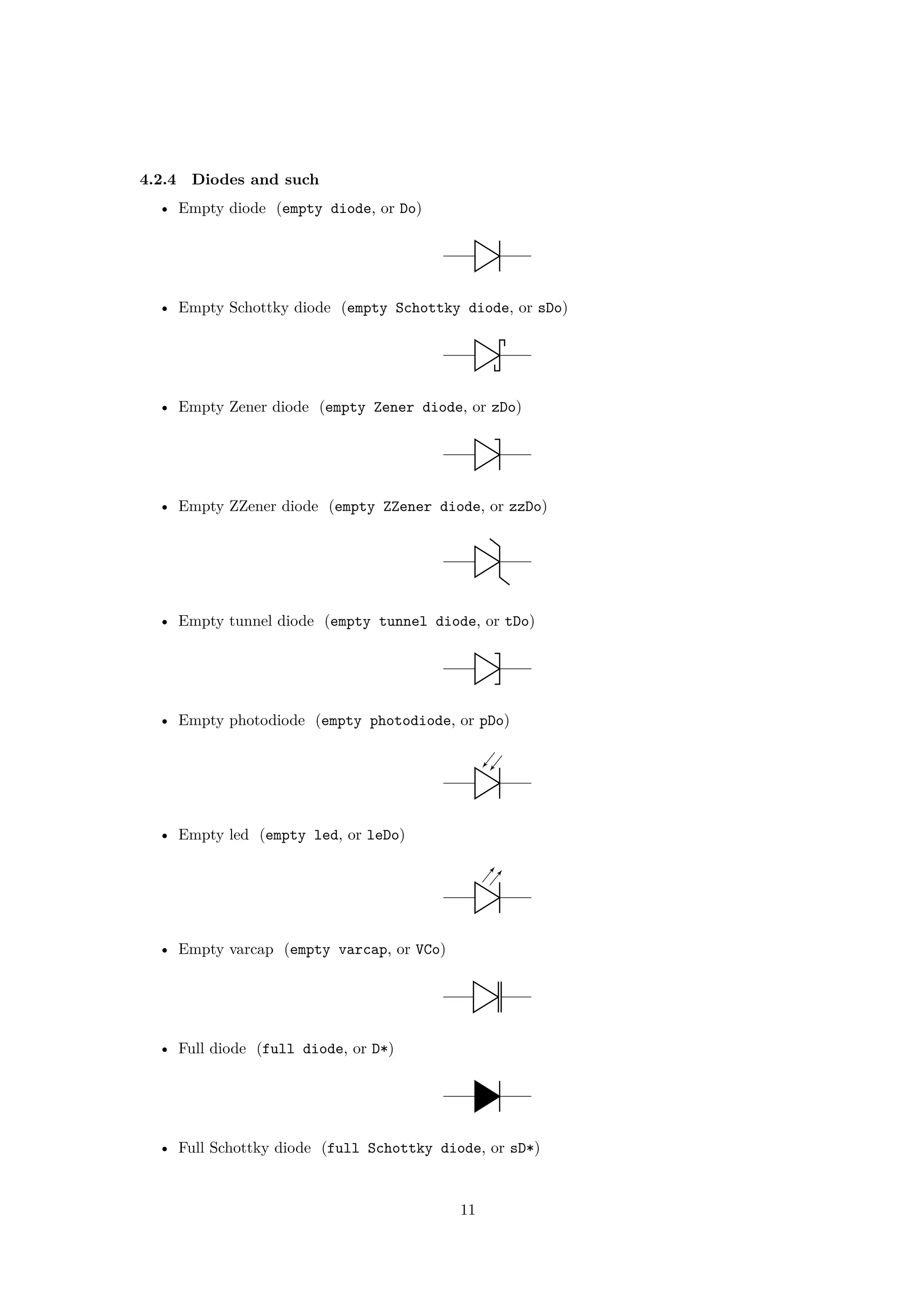
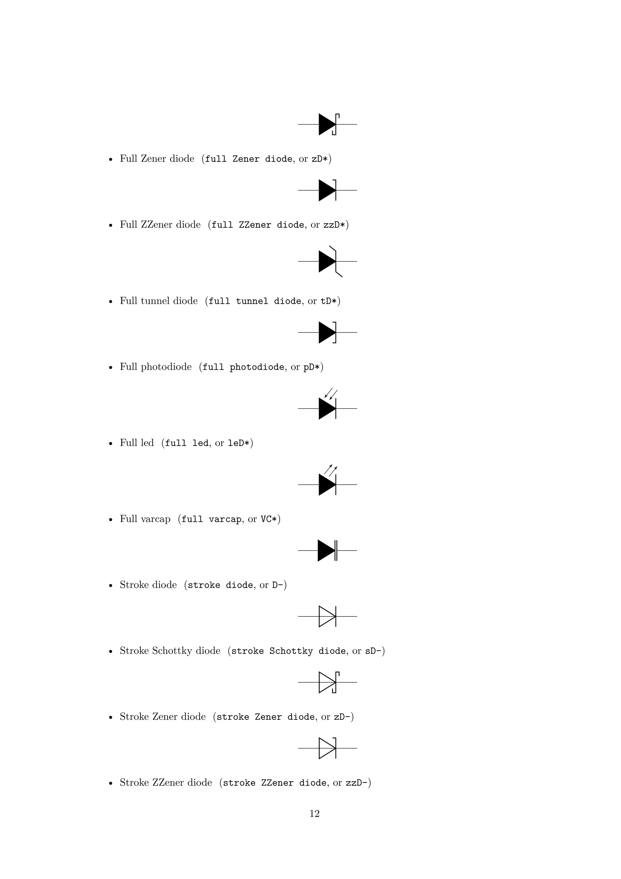
• Empty thyristor (empty thyristor, or Tyo)
• Full thyristor (full thyristor, or Ty*)
• Stroke thyristor (stroke thyristor, or Ty-)
See chapter 6.1.3 for information how access the third connector
The package options fulldiode, strokediode, and emptydiode (and the styles [full
diodes], [stroke diodes], and [empty diodes]) define which shape will be used by abbre-
viated commands such that D, sD, zD, zzD, tD, pD, leD, VC, Ty,Tr(no stroke symbol available!).
• Squid (squid)
• Barrier (barrier)
• European gas filled surge arrester (european gas filled surge arrester)
• American gas filled surge arrester (american gas filled surge arrester)
If (default behaviour) europeangfsurgearrester option is active (or the style [european
gas filled surge arrester] is used), the shorthands gas filled surge arrester and
gf surge arrester are equivalent to the european version of the component.
If otherwise americangfsurgearrester option is active (or the style [american gas
filled surge arrester] is used), the shorthands the shorthands gas filled surge
arrester and gf surge arrester are equivalent to the american version of the component.
14

4.2.6 Basic dynamical bipoles
• Capacitor (capacitor, or C)
• Polar capacitor (polar capacitor, or pC)
• Electrolytic capacitor (ecapacitor, or eC,elko)
+
• Variable capacitor (variable capacitor, or vC)
• Piezoelectric Element (piezoelectric, or PZ)
If (default behaviour) cuteinductors option is active (or the style [cute inductors] is used),
the inductors are displayed as follows:
• Inductor (L, or cute inductor)
• Variable inductor (vL, or variable cute inductor)
If americaninductors option is active (or the style [american inductors] is used), the
inductors are displayed as follows:
• Inductor (L, or american inductor)
• Variable inductor (vL, or variable american inductor)
15

Finally, if europeaninductors option is active (or the style [european inductors] is used),
the inductors are displayed as follows:
• Inductor (L, or european inductor)
• Variable inductor (vL, or variable european inductor)
There is also a transmission line:
• Transmission line (TL, or transmission line, tline)
4.2.7 Stationary sources
• Battery (battery)
• Single battery cell (battery1)
• Voltage source (european style) (european voltage source)
• Voltage source (american style) (american voltage source)
−
+
• Current source (european style) (european current source)
• Current source (american style) (american current source)
16

If (default behaviour) europeancurrents option is active (or the style [european
currents] is used), the shorthands current source, isource, and I are equivalent to
european current source. Otherwise, if americancurrents option is active (or the style
[american currents] is used) they are equivalent to american current source.
Similarly, if (default behaviour) europeanvoltages option is active (or the style
[european voltages] is used), the shorthands voltage source, vsource, and V are equiva-
lent to european voltage source. Otherwise, if americanvoltages option is active (or the
style [american voltages] is used) they are equivalent to american voltage source.
4.2.8 Sinusoidal sources
Here because I was asked for them. But how do you distinguish one from the other?!
• Sinusoidal voltage source (sinusoidal voltage source, or vsourcesin, sV)
• Sinusoidal current source (sinusoidal current source, or isourcesin, sI)
4.2.9 Special sources
• Square voltage source (square voltage source, or vsourcesquare, sqV)
• Triangle voltage source (vsourcetri, or tV)
• Empty voltage source (esource)
• Photovoltaic-voltage source (pvsource)
• Double Zero style current source (ioosource)
• Double Zero style voltage source (voosource)
17

4.2.10 DC sources
• DC voltage source (dcvsource)
• DC current source (dcisource)
4.2.11 Mechanical Analogy
• Mechanical Damping (damper)
• Mechanical Stiffness (spring)
• Mechanical Mass (mass)
4.2.12 Switch
• Switch (switch, or spst)
• Closing switch (closing switch, or cspst)
• Opening switch (opening switch, or ospst)
• Push button (push button)
18

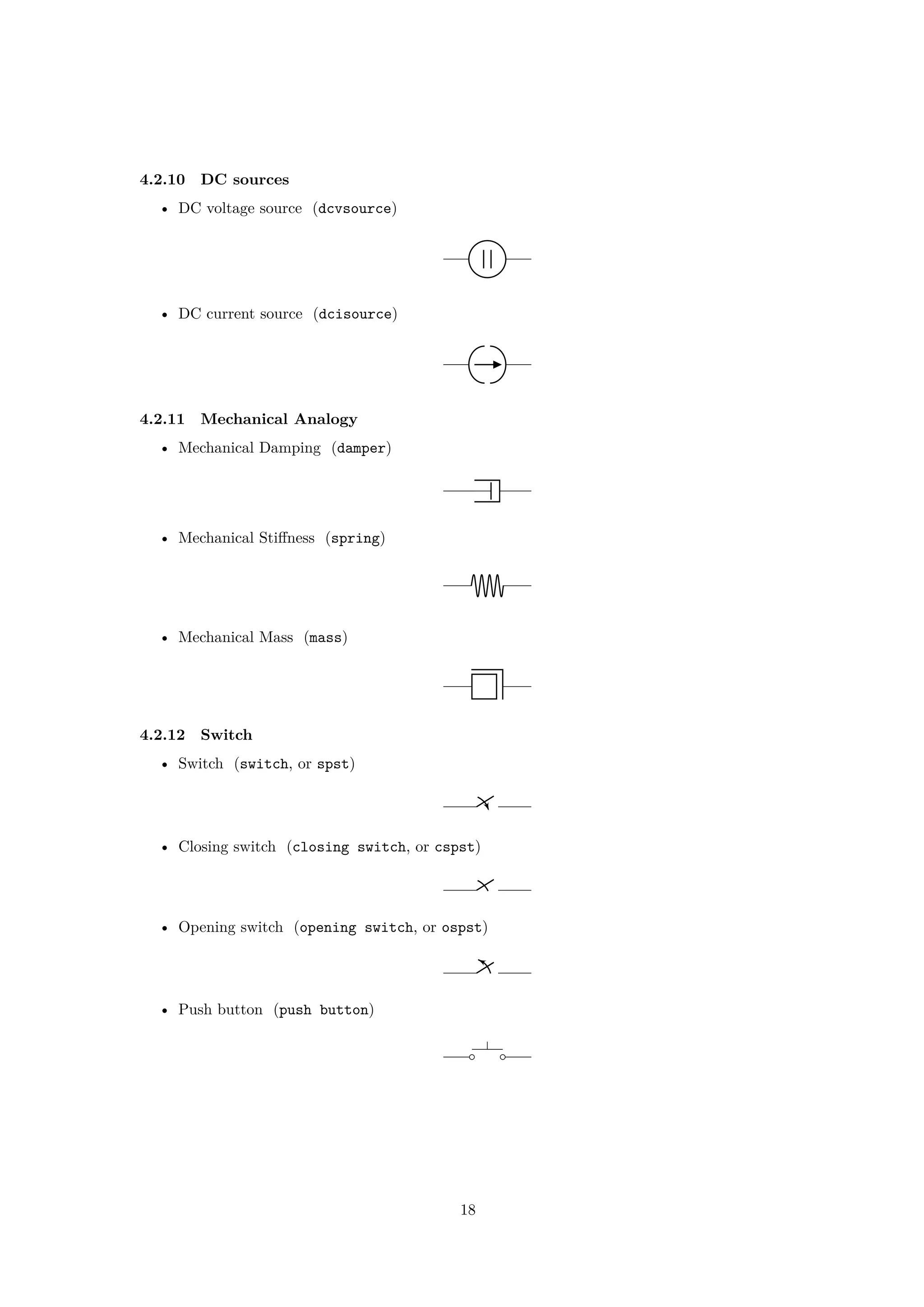
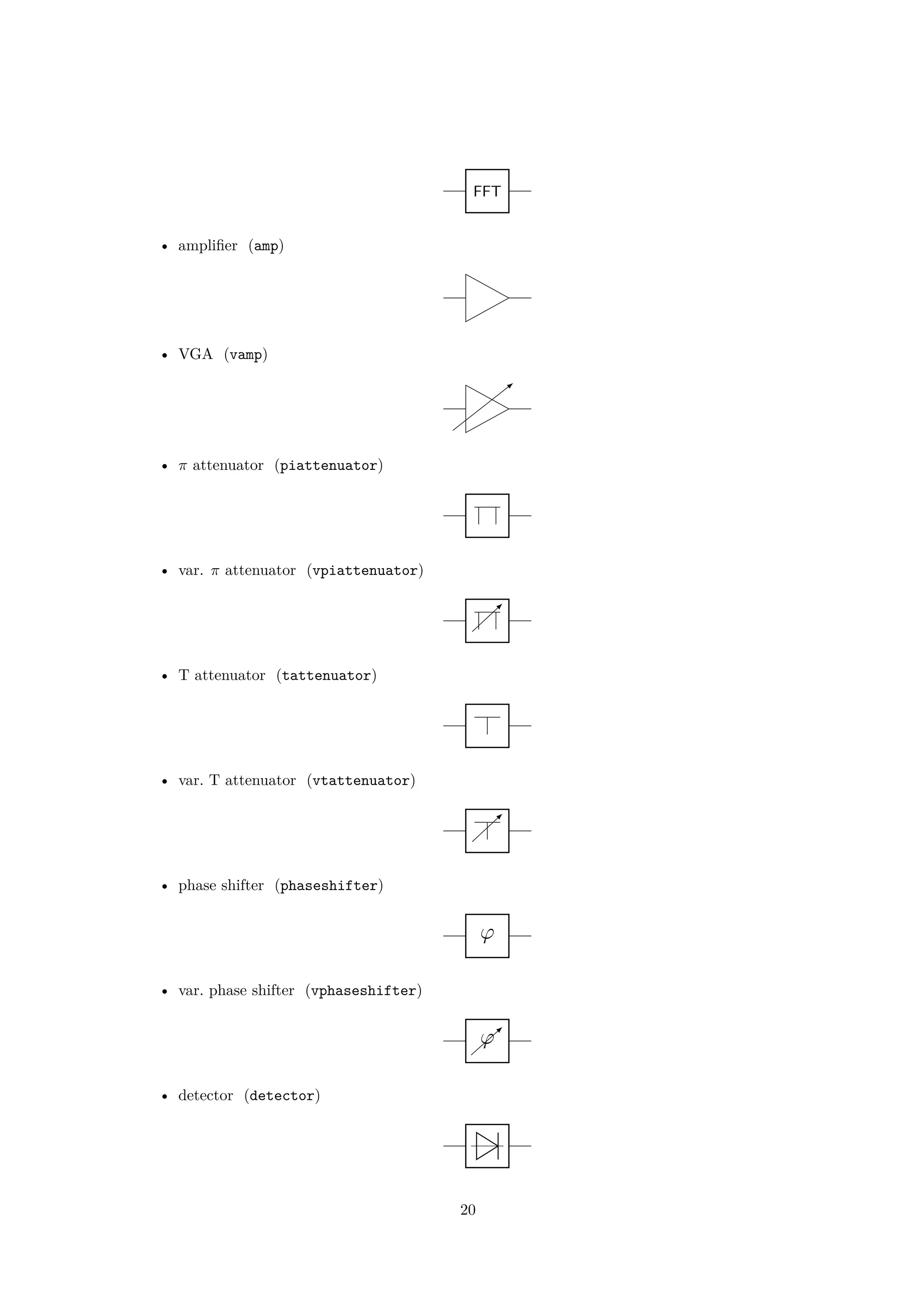
4.2.13 Block diagram components
Contributed by Stefan Erhardt.
• generic two port5
(twoport)
• vco (vco)
• bandpass (bandpass)
• highpass (highpass)
• lowpass (lowpass)
• A/D converter (adc)
A
D
• D/A converter (dac)
D
A
• DSP (dsp)
DSP
• FFT (fft)
5To specify text to be put in the component: twoport[t=text]):
text
19

FFT
• amplifier (amp)
• VGA (vamp)
• π attenuator (piattenuator)
• var. π attenuator (vpiattenuator)
• T attenuator (tattenuator)
• var. T attenuator (vtattenuator)
• phase shifter (phaseshifter)
φ
• var. phase shifter (vphaseshifter)
φ
• detector (detector)
20

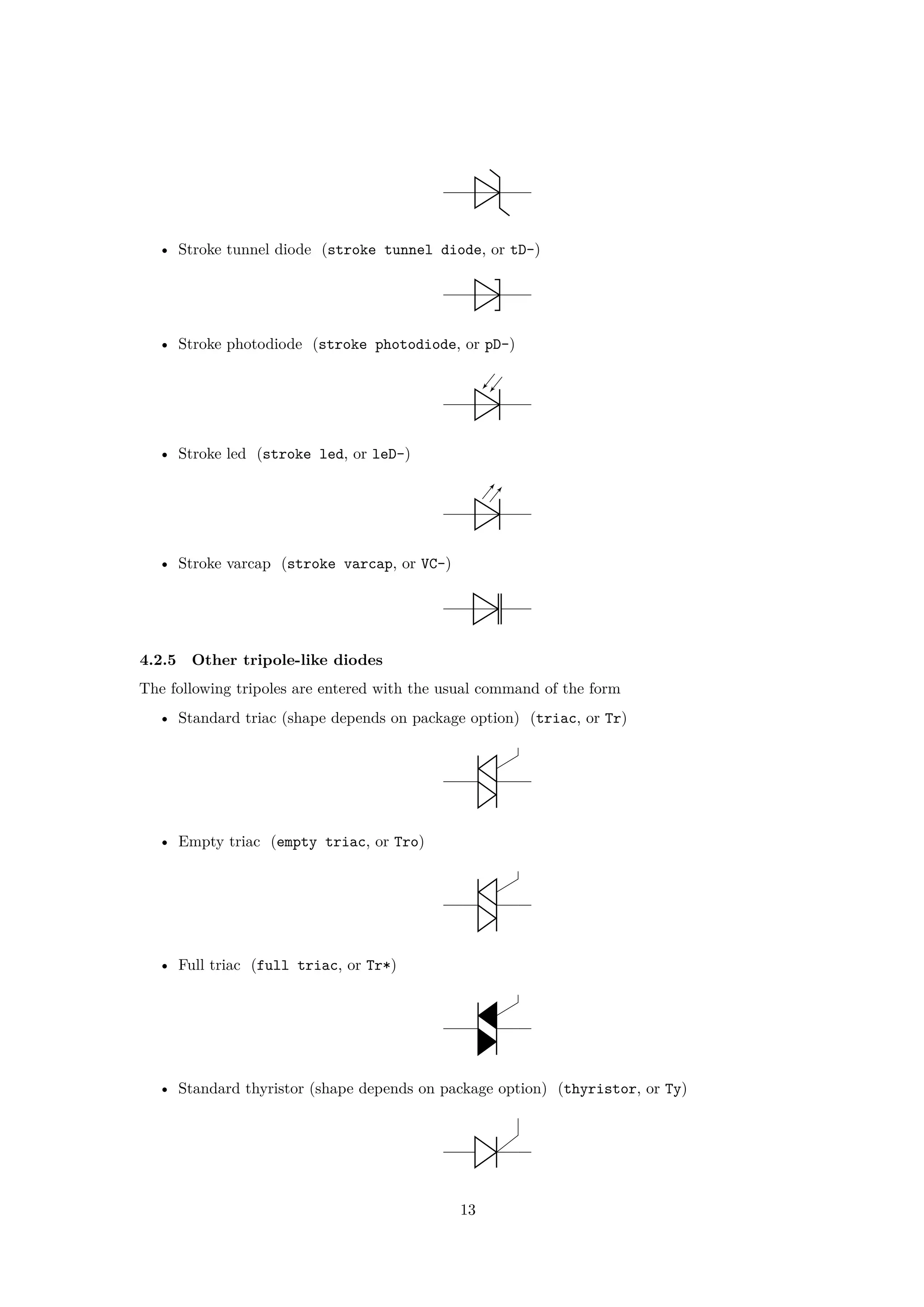
4.3 Tripoles
4.3.1 Controlled sources
Admittedly, graphically they are bipoles. But I couldn’t…
• Controlled voltage source (european style) (european controlled voltage source)
• Controlled voltage source (american style) (american controlled voltage source)
+
−
• Controlled current source (european style) (european controlled current source)
• Controlled current source (american style) (american controlled current source)
If (default behaviour) europeancurrents option is active (or the style [european
currents] is used), the shorthands controlled current source, cisource, and cI are
equivalent to european controlled current source. Otherwise, if americancurrents op-
tion is active (or the style [american currents] is used) they are equivalent to american
controlled current source.
Similarly, if (default behaviour) europeanvoltages option is active (or the style
[european voltages] is used), the shorthands controlled voltage source, cvsource,
and cV are equivalent to european controlled voltage source. Otherwise, if
americanvoltages option is active (or the style [american voltages] is used) they are
equivalent to american controlled voltage source.
• Controlled sinusoidal voltage source (controlled sinusoidal voltage source, or controlled
vsourcesin, cvsourcesin, csV)
• Controlled sinusoidal current source (controlled sinusoidal current source, or controlled
isourcesin, cisourcesin, csI)
21

4.3.2 Transistors
• nmos (node[nmos]{})
• pmos (node[pmos]{})
• npn (node[npn]{})
• pnp (node[pnp]{})
• npn (node[npn,photo]{})
• pnp (node[pnp,photo]{})
• nigbt (node[nigbt]{})
• pigbt (node[pigbt]{})
22

• Lnigbt (node[Lnigbt]{})
• Lpigbt (node[Lpigbt]{})
For all transistors a bodydiode(or freewheeling diode) can automatically be drawn. Just use
the global option bodydiode, or for single transistors, the tikz-option bodydiode:
1 begin{circuitikz}
2 draw (0,0) node[npn,bodydiode](npn){}++(2,0)node[pnp,
bodydiode](npn){};
3 draw (0,-2) node[nigbt,bodydiode](npn){}++(2,0)node[
pigbt,bodydiode](npn){};
4 draw (0,-4) node[nfet,bodydiode](npn){}++(2,0)node[
pfet,bodydiode](npn){};
5 end{circuitikz}
The Base/Gate connection of all transistors can be disable by using the options nogate or
nobase, respectively. The Base/Gate anchors are floating, but there an additional anchor ”no-
gate”/”nobase”, which can be used to point to the unconnected base:
E
C
B
1 begin{circuitikz}
2 draw (2,0) node[npn,nobase](npn){};
3 draw (npn.E) node[below]{E};
4 draw (npn.C) node[above]{C};
5 draw (npn.B) node[circ]{} node[left]{B};
6 draw[dashed,red,-latex] (1,0.5)--(npn.nobase);
7 end{circuitikz}
If the option arrowmos is used (or after the command ctikzset{tripoles/mos style/arrows}
is given), this is the output:
• nmos (node[nmos]{})
23

• pmos (node[pmos]{})
To draw the PMOS circle non-solid, use the option emptycircle or the command ctikzset{tripoles/pmos styl
• pmos (node[pmos,emptycircle]{})
nfets and pfets have been incorporated based on code provided by Clemens Helfmeier and
Theodor Borsche. Use the package options fetsolderdot/nofetsolderdot to enable/disable
solderdot at some fet-transistors. Additionally, the solderdot option can be enabled/disabled for
single transistors with the option ”solderdot” and ”nosolderdot”, respectively.
• nfet (node[nfet]{})
• nigfete (node[nigfete]{})
• nigfete (node[nigfete,solderdot]{})
• nigfetebulk (node[nigfetebulk]{})
24

• nigfetd (node[nigfetd]{})
• pfet (node[pfet]{})
• pigfete (node[pigfete]{})
• pigfetebulk (node[pigfetebulk]{})
• pigfetd (node[pigfetd]{})
njfet and pjfet have been incorporated based on code provided by Danilo Piazzalunga:
• njfet (node[njfet]{})
• pjfet (node[pjfet]{})
isfet
• isfet (node[isfet]{})
25

4.3.3 Block diagram
These come from Stefan Erhardt’s contribution of block diagram components. Add a box around
them with the option box.
• mixer (node[mixer]{})
• adder (node[adder]{})
• oscillator (node[oscillator]{})
• circulator (node[circulator]{})
• wilkinson divider (node[wilkinson]{})
4.3.4 Switch
• spdt (node[spdt]{})
• Toggle switch (toggle switch)
26

4.3.5 Electro-Mechanical Devices
• Motor (node[elmech]{M})
M
• Generator (node[elmech]{G})
G
M
ω
1 begin{circuitikz}
2 draw (2,0) node[elmech](motor){M};
3 draw (motor.north) |-(0,2) to [R] ++(0,-2) to[
dcvsource]++(0,-2) -| (motor.bottom);
4 draw[thick,->>](motor.right)--++(1,0)node[midway,
above]{$omega$};
5 end{circuitikz}
ω
1 begin{circuitikz}
2 draw (2,0) node[elmech](motor){};
3 draw (motor.north) |-(0,2) to [R] ++(0,-2) to[
dcvsource]++(0,-2) -| (motor.bottom);
4 draw[thick,->>](motor.center)--++(1.5,0)node[midway,
above]{$omega$};
5 end{circuitikz}
The symbols can also be used along a path, using the transistor-path-syntax(T in front of the
shape name, see section 6.6). Don´t forget to use parameter n to name the node and get acces to
the anchors:
M
M
G
ω
1 begin{circuitikz}
2 draw (0,0) to [Telmech=M,n=motor] ++(0,-3) to [
Telmech=M] ++(3,0) to [Telmech=G,n=generator]
++(0,3) to [R] (0,0);
3 draw[thick,->>](motor.left)--(generator.left)node[
midway,above]{$omega$};
4 end{circuitikz}
4.4 Double bipoles
Transformers automatically use the inductor shape currently selected. These are the three possi-
bilities:
27

• Transformer (cute inductor) (node[transformer]{})
• Transformer (american inductor) (node[transformer]{})
• Transformer (european inductor) (node[transformer]{})
Transformers with core are also available:
• Transformer core (cute inductor) (node[transformer core]{})
• Transformer core (american inductor) (node[transformer core]{})
• Transformer core (european inductor) (node[transformer core]{})
• Gyrator (node[gyrator]{})
28

• Coupler (node[coupler]{})
• Coupler, 2 (node[coupler2]{})
4.5 Logic gates
• American and port (node[american and port]{})
• American or port (node[american or port]{})
• American not port (node[american not port]{})
• American nand port (node[american nand port]{})
• American nor port (node[american nor port]{})
29

• American xor port (node[american xor port]{})
• American xnor port (node[american xnor port]{})
• European and port (node[european and port]{})
&
• European or port (node[european or port]{})
≥ 1
• European not port (node[european not port]{})
1
• European nand port (node[european nand port]{})
&
• European nor port (node[european nor port]{})
≥ 1
• European xor port (node[european xor port]{})
= 1
• European xnor port (node[european xnor port]{})
= 1
30

If (default behaviour) americanports option is active (or the style [american ports] is
used), the shorthands and port, or port, not port, nand port, not port, xor port, and
xnor port are equivalent to the american version of the respective logic port.
If otherwise europeanports option is active (or the style [european ports] is used), the
shorthands and port, or port, not port, nand port, not port, xor port, and xnor port
are equivalent to the european version of the respective logic port.
4.6 Amplifiers
• Operational amplifier (node[op amp]{})
−
+
• Fully differential operational amplifier6
(node[fd op amp]{})
−
+
−
+
• transconductance amplifier (node[gm amp]{})
−
+
• Plain amplifier (node[plain amp]{})
• Buffer (node[buffer]{})
6Contributed by Kristofer M. Monisit.
31

4.7 Support shapes
• Arrows (current and voltage) (node[currarrow]{})
• Arrow to draw at its tip, useful for block diagrams. (node[inputarrow]{})
• Connected terminal (node[circ]{})
• Unconnected terminal (node[ocirc]{})
5 Usage
R1
1 begin{circuitikz}
2 draw (0,0) to[R, l=$R_1$] (2,0);
3 end{circuitikz}
R1
1 begin{circuitikz}
2 draw (0,0) to[R=$R_1$] (2,0);
3 end{circuitikz}
i1
1 begin{circuitikz}
2 draw (0,0) to[R, i=$i_1$] (2,0);
3 end{circuitikz}
v1
1 begin{circuitikz}
2 draw (0,0) to[R, v=$v_1$] (2,0);
3 end{circuitikz}
R1
v1
i1
1 begin{circuitikz}
2 draw (0,0) to[R=$R_1$, i=$i_1$, v=$v_1$] (2,0);
3 end{circuitikz}
R1
v1
i1
1 begin{circuitikz}
2 draw (0,0) to[R=$R_1$, i=$i_1$, v=$v_1$] (2,0);
3 end{circuitikz}
Long names/styles for the bipoles can be used:
1 kΩ
1 begin{circuitikz}draw
2 (0,0) to[resistor=1<kiloohm>] (2,0)
3 ;end{circuitikz}
32

5.1 Labels
R1
1 begin{circuitikz}
2 draw (0,0) to[R, l^=$R_1$] (2,0);
3 end{circuitikz}
R1
1 begin{circuitikz}
2 draw (0,0) to[R, l_=$R_1$] (2,0);
3 end{circuitikz}
The default orientation of labels is controlled by the options smartlabels, rotatelabels and
straightlabels (or the corresponding label/align keys). Here are examples to see the differ-
ences:
0
4590
135
180
-90
-45
-135
1 begin{circuitikz}
2 ctikzset{label/align = straight}
3 defDIR{0,45,90,135,180,-90,-45,-135}
4 foreach i in DIR {
5 draw (0,0) to[R=i, *-o] (i:2.5);
6 }
7 end{circuitikz}
0
45
90
135
180
-90
-45
-135
1 begin{circuitikz}
2 ctikzset{label/align = rotate}
3 defDIR{0,45,90,135,180,-90,-45,-135}
5 draw (0,0) to[R=i, *-o] (i:2.5);
6 }
7 end{circuitikz}
0
45
90
135
180
-90
-45
-135
1 begin{circuitikz}
2 ctikzset{label/align = smart}
3 defDIR{0,45,90,135,180,-90,-45,-135}
5 draw (0,0) to[R=i, *-o] (i:2.5);
6 }
7 end{circuitikz}
33

5.2 Currents
The counting direction of currents and voltages have changed with version 0.5, for compability
reasons there is a option to use the olddirections(see options). For the new scheme, the following
rules apply:
• Normal bipoles: currents and voltages are counted positiv in drawing direction.
• Current Sources: current is counted positiv in drawing direction, voltage in opposite
direction
• Voltage Sources: voltage is counted positiv in drawing direction, current in opposite
direction
With this convention, the power at loads is positive and negative at sources.
i1
1 begin{circuitikz}
2 draw (0,0) to[R, i^>=$i_1$] (2,0);
3 end{circuitikz}
i1
1 begin{circuitikz}
2 draw (0,0) to[R, i_>=$i_1$] (2,0);
3 end{circuitikz}
i1
1 begin{circuitikz}
2 draw (0,0) to[R, i^<=$i_1$] (2,0);
3 end{circuitikz}
i1
1 begin{circuitikz}
2 draw (0,0) to[R, i_<=$i_1$] (2,0);
3 end{circuitikz}
i1
1 begin{circuitikz}
2 draw (0,0) to[R, i>^=$i_1$] (2,0);
3 end{circuitikz}
i1
1 begin{circuitikz}
2 draw (0,0) to[R, i>_=$i_1$] (2,0);
3 end{circuitikz}
i1
1 begin{circuitikz}
2 draw (0,0) to[R, i<^=$i_1$] (2,0);
3 end{circuitikz}
i1
1 begin{circuitikz}
2 draw (0,0) to[R, i<_=$i_1$] (2,0);
3 end{circuitikz}
Also
i1
1 begin{circuitikz}
2 draw (0,0) to[R, i<=$i_1$] (2,0);
3 end{circuitikz}
i1
1 begin{circuitikz}
2 draw (0,0) to[R, i>=$i_1$] (2,0);
3 end{circuitikz}
34

i1
1 begin{circuitikz}
2 draw (0,0) to[R, i^=$i_1$] (2,0);
3 end{circuitikz}
i1
1 begin{circuitikz}
2 draw (0,0) to[R, i_=$i_1$] (2,0);
3 end{circuitikz}
10V
i1
1 begin{circuitikz}
2 draw (0,0) to[V=10V, i_=$i_1$] (2,0);
3 end{circuitikz}
10V
i1
1 begin{circuitikz}
2 draw (0,0) to[V<=10V, i_=$i_1$] (2,0);
3 end{circuitikz}
−
+
10V
i1
1 begin{circuitikz}[american]
2 draw (0,0) to[V=10V, i_=$i_1$] (2,0);
3 end{circuitikz}
+
−
10V
i1
1 begin{circuitikz}[american]
2 draw (0,0) to[V<=10V, i_=$i_1$] (2,0);
3 end{circuitikz}
5.3 Voltages
See introduction note at Currents (chapter 5.2, page 32)!
5.3.1 European style
The default, with arrows. Use option europeanvoltage or style [european voltages].
v1
1 begin{circuitikz}[european voltages]
2 draw (0,0) to[R, v^>=$v_1$] (2,0);
3 end{circuitikz}
v1
2 draw (0,0) to[R, v^<=$v_1$] (2,0);
3 end{circuitikz}
v1
2 draw (0,0) to[R, v_>=$v_1$] (2,0);
3 end{circuitikz}
v1
2 draw (0,0) to[R, v_<=$v_1$] (2,0);
3 end{circuitikz}
10V
i1
1 begin{circuitikz}
2 draw (0,0) to[V=10V, i_=$i_1$] (2,0);
3 end{circuitikz}
35

10V
i1
1 begin{circuitikz}
2 draw (0,0) to[V<=10V, i_=$i_1$] (2,0);
3 end{circuitikz}
u1
1A
1 begin{circuitikz}
2 draw (0,0) to[I=1A, v_=$u_1$] (2,0);
3 end{circuitikz}
i1
1A
1 begin{circuitikz}
2 draw (0,0) to[I<=1A, v_=$i_1$] (2,0);
3 end{circuitikz}
5.3.2 American style
For those who like it (not me). Use option americanvoltage or set [american voltages].
+ −v1
1 begin{circuitikz}[american voltages]
2 draw (0,0) to[R, v^>=$v_1$] (2,0);
3 end{circuitikz}
− +v1
2 draw (0,0) to[R, v^<=$v_1$] (2,0);
3 end{circuitikz}
+ −v1
2 draw (0,0) to[R, v_>=$v_1$] (2,0);
3 end{circuitikz}
− +v1
2 draw (0,0) to[R, v_<=$v_1$] (2,0);
3 end{circuitikz}
− +
u1
1A 1 begin{circuitikz}[american]
2 draw (0,0) to[I=1A, v_=$u_1$] (2,0);
3 end{circuitikz}
+ −
i1
1A 1 begin{circuitikz}[american]
2 draw (0,0) to[I<=1A, v_=$i_1$] (2,0);
3 end{circuitikz}
5.4 Nodes
1 begin{circuitikz}
2 draw (0,0) to[R, o-o] (2,0);
3 end{circuitikz}
1 begin{circuitikz}
2 draw (0,0) to[R, -o] (2,0);
3 end{circuitikz}
36

1 begin{circuitikz}
2 draw (0,0) to[R, o-] (2,0);
3 end{circuitikz}
1 begin{circuitikz}
2 draw (0,0) to[R, *-*] (2,0);
3 end{circuitikz}
1 begin{circuitikz}
2 draw (0,0) to[R, -*] (2,0);
3 end{circuitikz}
1 begin{circuitikz}
2 draw (0,0) to[R, *-] (2,0);
3 end{circuitikz}
1 begin{circuitikz}
2 draw (0,0) to[R, d-d] (2,0);
3 end{circuitikz}
1 begin{circuitikz}
2 draw (0,0) to[R, -d] (2,0);
3 end{circuitikz}
1 begin{circuitikz}
2 draw (0,0) to[R, d-] (2,0);
3 end{circuitikz}
1 begin{circuitikz}
2 draw (0,0) to[R, o-*] (2,0);
3 end{circuitikz}
1 begin{circuitikz}
2 draw (0,0) to[R, *-o] (2,0);
3 end{circuitikz}
1 begin{circuitikz}
2 draw (0,0) to[R, o-d] (2,0);
3 end{circuitikz}
1 begin{circuitikz}
2 draw (0,0) to[R, d-o] (2,0);
3 end{circuitikz}
1 begin{circuitikz}
2 draw (0,0) to[R, *-d] (2,0);
3 end{circuitikz}
1 begin{circuitikz}
2 draw (0,0) to[R, d-*] (2,0);
3 end{circuitikz}
37

5.5 Special components
For some components label, current and voltage behave as one would expect:
a1 1 begin{circuitikz}
2 draw (0,0) to[I=$a_1$] (2,0);
3 end{circuitikz}
2 draw (0,0) to[I, i=$a_1$] (2,0);
3 end{circuitikz}
k · a1 1 begin{circuitikz}
2 draw (0,0) to[cI=$kcdot a_1$] (2,0);
3 end{circuitikz}
2 draw (0,0) to[sI=$a_1$] (2,0);
3 end{circuitikz}
k · a1 1 begin{circuitikz}
2 draw (0,0) to[csI=$kcdot a_1$] (2,0);
3 end{circuitikz}
The following results from using the option americancurrent or using the style [american currents].
a1 1 begin{circuitikz}[american currents]
2 draw (0,0) to[I=$a_1$] (2,0);
3 end{circuitikz}
2 draw (0,0) to[I, i=$a_1$] (2,0);
3 end{circuitikz}
k · a1 1 begin{circuitikz}[american currents]
2 draw (0,0) to[cI=$kcdot a_1$] (2,0);
3 end{circuitikz}
2 draw (0,0) to[sI=$a_1$] (2,0);
3 end{circuitikz}
k · a1 1 begin{circuitikz}[american currents]
2 draw (0,0) to[csI=$kcdot a_1$] (2,0);
3 end{circuitikz}
The same holds for voltage sources:
38

2 draw (0,0) to[V=$a_1$] (2,0);
3 end{circuitikz}
2 draw (0,0) to[V, v=$a_1$] (2,0);
3 end{circuitikz}
k · a1
1 begin{circuitikz}
2 draw (0,0) to[cV=$kcdot a_1$] (2,0);
3 end{circuitikz}
2 draw (0,0) to[sV=$a_1$] (2,0);
3 end{circuitikz}
k · a1
1 begin{circuitikz}
2 draw (0,0) to[csV=$kcdot a_1$] (2,0);
3 end{circuitikz}
The following results from using the option americanvoltage or the style [american voltages].
−
+
a1 1 begin{circuitikz}[american voltages]
2 draw (0,0) to[V=$a_1$] (2,0);
3 end{circuitikz}
−
+
a1 1 begin{circuitikz}[american voltages]
2 draw (0,0) to[V, v=$a_1$] (2,0);
3 end{circuitikz}
+
−
k · a1 1 begin{circuitikz}[american voltages]
2 draw (0,0) to[cV=$kcdot a_1$] (2,0);
3 end{circuitikz}
+ −a1 1 begin{circuitikz}[american voltages]
2 draw (0,0) to[sV=$a_1$] (2,0);
3 end{circuitikz}
+ −k · a1 1 begin{circuitikz}[american voltages]
2 draw (0,0) to[csV=$kcdot a_1$] (2,0);
3 end{circuitikz}
5.6 Integration with siunitx
If the option siunitx is active (and not in ConTEXt), then the following are equivalent:
1 kΩ
1 begin{circuitikz}
2 draw (0,0) to[R, l=1<kiloohm>] (2,0);
3 end{circuitikz}
39

1 kΩ
1 begin{circuitikz}
2 draw (0,0) to[R, l=$SI{1}{kiloohm}$] (2,0);
3 end{circuitikz}
1 mA
1 begin{circuitikz}
2 draw (0,0) to[R, i=1<milliampere>] (2,0);
3 end{circuitikz}
1 mA
1 begin{circuitikz}
2 draw (0,0) to[R, i=$SI{1}{milliampere}$] (2,0);
3 end{circuitikz}
1 V
1 begin{circuitikz}
2 draw (0,0) to[R, v=1<volt>] (2,0);
3 end{circuitikz}
1 V
1 begin{circuitikz}
2 draw (0,0) to[R, v=$SI{1}{volt}$] (2,0);
3 end{circuitikz}
5.7 Mirroring
1 begin{circuitikz}
2 draw (0,0) to[pD] (2,0);
3 end{circuitikz}
1 begin{circuitikz}
2 draw (0,0) to[pD, mirror] (2,0);
3 end{circuitikz}
At the moment, placing labels and currents on mirrored bipoles works:
T
1 begin{circuitikz}
2 draw (0,0) to[ospst=T] (2,0);
3 end{circuitikz}
T
i1 1 begin{circuitikz}
2 draw (0,0) to[ospst=T, mirror, i=$i_1$] (2,0);
3 end{circuitikz}
But voltages don’t:
T
v 1 begin{circuitikz}
2 draw (0,0) to[ospst=T, mirror, v=v] (2,0);
3 end{circuitikz}
Sorry about that.
5.8 Putting them together
1 kΩ
1 mA
1 begin{circuitikz}
2 draw (0,0) to[R=1<kiloohm>,
3 i>_=1<milliampere>, o-*] (3,0);
4 end{circuitikz}
vD
1 mA
1 begin{circuitikz}
2 draw (0,0) to[D*, v=$v_D$,
3 i=1<milliampere>, o-*] (3,0);
4 end{circuitikz}
40

6 Not only bipoles
Since only bipoles (but see section 6.6) can be placed ”along a line”, components with more than
two terminals are placed as nodes:
+5 V
-5 V
1 begin{circuitikz}
2 draw (0,0) node[npn](npn) at (0,0) {};
3 draw (npn.C) --++(0,0.5) node[vcc]{+5,textnormal{V}};
4 draw (npn.E) --++(0,-0.5) node[vee]{-5,textnormal{V}};
5 end{circuitikz}
6.1 Anchors
In order to allow connections with other components, all components define anchors.
6.1.1 Logical ports
All logical ports, except not, have two inputs and one output. They are called respectively in 1,
in 2, out:
1
2
3
1 begin{circuitikz} draw
2 (0,0) node[and port] (myand) {}
3 (myand.in 1) node[anchor=east] {1}
4 (myand.in 2) node[anchor=east] {2}
5 (myand.out) node[anchor=west] {3}
6 ;end{circuitikz}
2 (0,2) node[and port] (myand1) {}
4 (2,1) node[xnor port] (myxnor) {}
5 (myand1.out) -| (myxnor.in 1)
7 ;end{circuitikz}
In the case of not, there are only in and out (although for compatibility reasons in 1 is still
defined and equal to in):
2 (1,0) node[not port] (not1) {}
3 (3,0) node[not port] (not2) {}
4 (0,0) -- (not1.in)
5 (not2.in) -- (not1.out)
6 ++(0,-1) node[ground] {} to[C] (not1.out)
7 (not2.out) -| (4,1) -| (0,0)
8 ;end{circuitikz}
41

6.1.2 Transistors
For nmos, pmos, nfet, nigfete, nigfetd, pfet, pigfete, and pigfetd transistors one has
base, gate, source and drain anchors (which can be abbreviated with B, G, S and D):
G
D
S
2 (0,0) node[nmos] (mos) {}
3 (mos.gate) node[anchor=east] {G}
4 (mos.drain) node[anchor=south] {D}
5 (mos.source) node[anchor=north] {S}
6 ;end{circuitikz}
G
D
S
Bulk
2 (0,0) node[pigfete] (pigfete) {}
3 (pigfete.G) node[anchor=east] {G}
4 (pigfete.D) node[anchor=north] {D}
5 (pigfete.S) node[anchor=south] {S}
6 (pigfete.bulk) node[anchor=east] {Bulk}
7 ;end{circuitikz}
Similarly njfet and pjfet have gate, source and drain anchors (which can be abbreviated
with G, S and D):
G
D
S 1 begin{circuitikz} draw
2 (0,0) node[pjfet] (pjfet) {}
3 (pjfet.G) node[anchor=east] {G}
4 (pjfet.D) node[anchor=north] {D}
5 (pjfet.S) node[anchor=south] {S}
6 ;end{circuitikz}
For npn, pnp, nigbt, and pigbt transistors the anchors are base, emitter and collector
anchors (which can be abbreviated with B, E and C):
B
C
E
2 (0,0) node[npn] (npn) {}
3 (npn.base) node[anchor=east] {B}
4 (npn.collector) node[anchor=south] {C}
5 (npn.emitter) node[anchor=north] {E}
6 ;end{circuitikz}
B
C
E 1 begin{circuitikz} draw
2 (0,0) node[pigbt] (pigbt) {}
3 (pigbt.B) node[anchor=east] {B}
4 (pigbt.C) node[anchor=north] {C}
5 (pigbt.E) node[anchor=south] {E}
6 ;end{circuitikz}
Here is one composite example (please notice that the xscale=-1 style would also reflect the
label of the transistors, so here a new node is added and its text is used, instead of that of pnp1):
42

2
1
2 (0,0) node[pnp] (pnp2) {2}
3 (pnp2.B) node[pnp, xscale=-1, anchor=B] (pnp1) {}
4 (pnp1) node {1}
5 (pnp1.C) node[npn, anchor=C] (npn1) {}
6 (pnp2.C) node[npn, xscale=-1, anchor=C] (npn2) {}
7 (pnp1.E) -- (pnp2.E) (npn1.E) -- (npn2.E)
8 (pnp1.B) node[circ] {} |- (pnp2.C) node[circ] {}
9 ;end{circuitikz}
Similarly, transistors and other components can be reflected vertically:
Bulk
G
D
S
2 (0,0) node[pigfete, yscale=-1] (pigfete) {}
3 (pigfete.bulk) node[anchor=west] {Bulk}
4 (pigfete.G) node[anchor=east] {G}
5 (pigfete.D) node[anchor=south] {D}
6 (pigfete.S) node[anchor=north] {S}
7 ;end{circuitikz}
R1
1 begin{circuitikz}
2 draw (0,2)
3 node[rground, yscale=-1]
{}
4 to[R=$R_1$] (0,0)
5 node[sground] {};
6 end{circuitikz}
6.1.3 Other tripoles
When inserting a thrystor, a triac or a potentiometer, one needs to refer to the third node–gate
(gate or G) for the former two; wiper (wiper or W) for the latter one. This is done by giving a
name to the bipole:
2 (0,0) to[Tr, n=TRI] (2,0)
3 to[pR, n=POT] (4,0);
4 draw[dashed] (TRI.G) -| (POT.wiper)
5 ;end{circuitikz}
As for the switches:
in
out 1
out 2
2 (0,0) node[spdt] (Sw) {}
3 (Sw.in) node[left] {in}
4 (Sw.out 1) node[right] {out 1}
5 (Sw.out 2) node[right] {out 2}
6 ;end{circuitikz}
2 (0,0) to[C] (1,0) to[toggle switch , n=Sw] (2.5,0)
3 -- (2.5,-1) to[battery1] (1.5,-1) to[R] (0,-1) -| (0,0)
4 (Sw.out 2) -| (2.5, 1) to[R] (0,1) -- (0,0)
5 ;end{circuitikz}
43

The ports of the mixer and adder can be addressed with numbers or west/south/east/north:
1
2
3
4
2 (0,0) node[mixer] (mix) {}
3 (mix.1) node[left] {1}
4 (mix.2) node[below] {2}
5 (mix.3) node[right] {3}
6 (mix.4) node[above] {4}
7 ;end{circuitikz}
The Wilkinson divider has:
3 dB
in
out1
out2
2 (0,0) node[wilkinson] (w) {SI{3}{dB}}
3 (w.in) to[short,-o] ++(-0.5,0)
4 (w.out1) to[short,-o] ++(0.5,0)
5 (w.out2) to[short,-o] ++(0.5,0)
6 (w.in) node[below left] {texttt{in}}
7 (w.out1) node[below right] {texttt{out1}}
8 (w.out2) node[above right] {texttt{out2}}
9 ;
10 end{circuitikz}
6.1.4 Operational amplifier
The op amp defines the inverting input (-), the non-inverting input (+) and the output (out)
anchors:
−
+v+
v−
vo
5 V
-5 V
2 (0,0) node[op amp] (opamp) {}
3 (opamp.+) node[left] {$v_+$}
4 (opamp.-) node[left] {$v_-$}
5 (opamp.out) node[right] {$v_o$}
6 (opamp.up) --++(0,0.5) node[vcc]{5,textnormal{V}}
7 (opamp.down) --++(0,-0.5) node[vee]{-5,textnormal{V
}}
8 ;end{circuitikz}
There are also two more anchors defined, up and down, for the power supplies:
−
+v+
v−
vo
12 V
2 (0,0) node[op amp] (opamp) {}
5 (opamp.out) node[right] {$v_o$}
6 (opamp.down) node[ground] {}
7 (opamp.up) ++ (0,.5) node[above] {SI{12}{volt}}
8 -- (opamp.up)
9 ;end{circuitikz}
The fully differential op amp defines two outputs:
44

−
+
−
+
v+
v− out +
out -
2 (0,0) node[fd op amp] (opamp) {}
5 (opamp.out +) node[right] {out +}
6 (opamp.out -) node[right] {out -}
7 (opamp.down) node[ground] {}
8 ;end{circuitikz}
6.1.5 Double bipoles
All the (few, actually) double bipoles/quadrupoles have the four anchors, two for each port. The
first port, to the left, is port A, having the anchors A1 (up) and A2 (down); same for port B. They
also expose the base anchor, for labelling:
A1
A2
B1
B2
K
2 (0,0) node[transformer] (T) {}
3 (T.A1) node[anchor=east] {A1}
4 (T.A2) node[anchor=east] {A2}
5 (T.B1) node[anchor=west] {B1}
6 (T.B2) node[anchor=west] {B2}
7 (T.base) node{K}
8 ;end{circuitikz}
A1
A2
B1
B2
K
2 (0,0) node[gyrator] (G) {}
3 (G.A1) node[anchor=east] {A1}
4 (G.A2) node[anchor=east] {A2}
5 (G.B1) node[anchor=west] {B1}
6 (G.B2) node[anchor=west] {B2}
7 (G.base) node{K}
8 ;end{circuitikz}
However:
10 dB
1 2
34
2 (0,0) node[coupler] (c) {SI{10}{dB}}
3 (c.1) to[short,-o] ++(-0.5,0)
4 (c.2) to[short,-o] ++(0.5,0)
5 (c.3) to[short,-o] ++(0.5,0)
6 (c.4) to[short,-o] ++(-0.5,0)
7 (c.1) node[below left] {texttt{1}}
8 (c.2) node[below right] {texttt{2}}
9 (c.3) node[above right] {texttt{3}}
10 (c.4) node[above left] {texttt{4}}
11 ;
12 end{circuitikz}
45

3 dB
1 2
34
2 (0,0) node[coupler2] (c) {SI{3}{dB}}
3 (c.1) to[short,-o] ++(-0.5,0)
4 (c.2) to[short,-o] ++(0.5,0)
5 (c.3) to[short,-o] ++(0.5,0)
6 (c.4) to[short,-o] ++(-0.5,0)
7 (c.1) node[below left] {texttt{1}}
8 (c.2) node[below right] {texttt{2}}
9 (c.3) node[above right] {texttt{3}}
10 (c.4) node[above left] {texttt{4}}
11 ;
12 end{circuitikz}
6.2 Input arrows
Two ports
With the option > you can draw an arrow to the input of the block diagram symbols.
A
D
2 (0,0) to[short,o-] ++(0.3,0)
3 to[lowpass,>] ++(2,0)
4 to[adc,>] ++(2,0)
5 to[short,-o] ++(0.3,0);
6 end{circuitikz}
Multi ports
Since inputs and outputs can vary, input arrows can be placed as nodes. Note that you have to
rotate the arrow on your own:
2 (0,0) node[mixer] (m) {}
3 (m.1) to[short,-o] ++(-1,0)
4 (m.2) to[short,-o] ++(0,-1)
5 (m.3) to[short,-o] ++(1,0)
6 (m.1) node[inputarrow] {}
7 (m.2) node[inputarrow,rotate=90] {};
8 end{circuitikz}
6.3 Labels and custom twoport boxes
Some twoports have the option to place a normal label (l=) and a inner label (t=).
LNA
F=0.9 dB
1 begin{circuitikz}
2 ctikzset{bipoles/amp/width=0.9}
3 draw (0,0) to[amp,t=LNA,l_=$F{=}0.9,$dB,o-o] ++(3,0);
4 end{circuitikz}
6.4 Box option
Some devices have the possibility to add a box around them. The inner symbol scales down to fit
inside the box.
46

2 (0,0) node[mixer,box,anchor=east] (m) {}
3 to[amp,box,>,-o] ++(2.5,0)
4 (m.west) node[inputarrow] {} to[short,-o]
++(-0.8,0)
5 (m.south) node[inputarrow,rotate=90] {} --
6 ++(0,-0.7) node[oscillator,box,anchor=north] {};
7 end{circuitikz}
6.5 Dash optional parts
To show that a device is optional, you can dash it. The inner symbol will be kept with solid lines.
10 dB opt.
1 begin{circuitikz}
2 draw (0,0) to[amp,l=SI{10}{dB}] ++(2.5,0);
3 draw[dashed] (2.5,0) to[lowpass,l=opt.]
++(2.5,0);
4 end{circuitikz}
6.6 Transistor paths
For syntactical convenience transistors can be placed using the normal path notation used for
bipoles. The transitor type can be specified by simply adding a “T” (for transistor) in front of the
node name of the transistor. It will be placed with the base/gate orthogonal to the direction of
the path:
1
2 3 1 begin{circuitikz} draw
2 (0,0) node[njfet] {1}
3 (-1,2) to[Tnjfet=2] (1,2)
4 to[Tnjfet=3, mirror] (3,2);
5 ;end{circuitikz}
Access to the gate and/or base nodes can be gained by naming the transistors with the n or
name path style:
1 begin{circuitikz} draw[yscale=1.1, xscale=.8]
2 (2,4.5) -- (0,4.5) to[Tpmos, n=p1] (0,3)
3 to[Tnmos, n=n1] (0,1.5)
4 to[Tnmos, n=n2] (0,0) node[ground] {}
5 (2,4.5) to[Tpmos,n=p2] (2,3) to[short, -*] (0,3)
6 (p1.G) -- (n1.G) to[short, *-o] ($(n1.G)+(3,0)$)
7 (n2.G) ++(2,0) node[circ] {} -| (p2.G)
8 (n2.G) to[short, -o] ($(n2.G)+(3,0)$)
9 (0,3) to[short, -o] (-1,3)
10 ;end{circuitikz}
The name property is available also for bipoles, although this is useful mostly for triac, poten-
tiometer and thyristor (see 4.2.5).
47

7 Customization
7.1 Parameters
Pretty much all CircuiTikZ relies heavily on pgfkeys for value handling and configuration. Indeed,
at the beginning of circuitikz.sty a series of key definitions can be found that modify all the
graphical characteristics of the package.
All can be varied using the ctikzset command, anywhere in the code.
Shape of the components (on a per-component-class basis)
1 Ω
1 Ω
1 tikz draw (0,0) to[R=1<ohm>] (2,0); par
2 ctikzset{bipoles/resistor/height=.6}
3 tikz draw (0,0) to[R=1<ohm>] (2,0);
1 tikz draw (0,0) node[nand port] {}; par
2 ctikzset{tripoles/american nand port/input height=.2}
3 ctikzset{tripoles/american nand port/port width=.2}
4 tikz draw (0,0) node[nand port] {};
Thickness of the lines (globally)
1 F
1 F
1 tikz draw (0,0) to[C=1<farad>] (2,0); par
2 ctikzset{bipoles/thickness=1}
3 tikz draw (0,0) to[C=1<farad>] (2,0);
Global properties Of voltage and current
1 V
1 V
1 tikz draw (0,0) to[R, v=1<volt>] (2,0); par
2 ctikzset{voltage/distance from node=.1}
3 tikz draw (0,0) to[R, v=1<volt>] (2,0);
ı
ı
1 tikz draw (0,0) to[C, i=$imath$] (2,0); par
2 ctikzset{current/distance = .2}
3 tikz draw (0,0) to[C, i=$imath$] (2,0);
However, you can override the properties voltage/distance from node7
, voltage/bump b8
and
voltage/european label distance9
on a per-component basis, in order to fine-tune the voltages:
7That is, how distant from the initial and final points of the path the arrow starts and ends.
8Controlling how high the bump of the arrow is — how curved it is.
9Controlling how distant from the bipole the voltage label will be.
48

1 V
2 V
1 V
2 V
1 tikz draw (0,0) to[R, v=1<volt>] (1.5,0)
2 to[C, v=2<volt>] (3,0); par
3 ctikzset{bipoles/capacitor/voltage/%
4 distance from node/.initial=.7}
5 tikz draw (0,0) to[R, v=1<volt>] (1.5,0)
6 to[C, v=2<volt>] (3,0); par
Admittedly, not all graphical properties have understandable names, but for the time it will have
to do:
1 tikz draw (0,0) node[xnor port] {};
2 ctikzset{tripoles/american xnor port/aaa=.2}
3 ctikzset{tripoles/american xnor port/bbb=.6}
4 tikz draw (0,0) node[xnor port] {};
7.2 Components size
Perhaps the most important parameter is circuitikzbasekey/bipoles/length, which can be
interpreted as the length of a resistor (including reasonable connections): all other lenghts are
relative to this value. For instance:
B
20 Ω
10 Ω
vx
S
5 vx5 Ω
A
1 ctikzset{bipoles/length=1.4cm}
2 begin{circuitikz}[scale=1.2]draw
3 (0,0) node[anchor=east] {B}
4 to[short, o-*] (1,0)
5 to[R=20<ohm>, *-*] (1,2)
6 to[R=10<ohm>, v=$v_x$] (3,2) -- (4,2)
7 to[cI=$frac{si{siemens}}{5} v_x$, *-*] (4,0) -- (3,0)
8 to[R=5<ohm>, *-*] (3,2)
9 (3,0) -- (1,0)
10 (1,2) to[short, -o] (0,2) node[anchor=east]{A}
11 ;end{circuitikz}
49

B
20 Ω
10 Ω
vx
S
5 vx5 Ω
A
1 ctikzset{bipoles/length=.8cm}
4 to[short, o-*] (1,0)
5 to[R=20<ohm>, *-*] (1,2)
6 to[R=10<ohm>, v=$v_x$] (3,2) -- (4,2)
7 to[cI=$frac{siemens}{5} v_x$, *-*] (4,0) -- (3,0)
8 to[R=5<ohm>, *-*] (3,2)
9 (3,0) -- (1,0)
11 ;end{circuitikz}
7.3 Colors
The color of the components is stored in the key circuitikzbasekey/color. CircuiTikZ tries to
follow the color set in TikZ, although sometimes it fails. If you change color in the picture, please
do not use just the color name as a style, like [red], but rather assign the style [color=red].
Compare for instance
1 begin{circuitikz} draw[red]
7 ;end{circuitikz}
and
1 begin{circuitikz} draw[color=red]
7 ;end{circuitikz}
One can of course change the color in medias res:
50

2 (0,0) node[pnp, color=blue] (pnp2) {}
3 (pnp2.B) node[pnp, xscale=-1, anchor=B, color=brown] (pnp1) {}
4 (pnp1.C) node[npn, anchor=C, color=green] (npn1) {}
5 (pnp2.C) node[npn, xscale=-1, anchor=C, color=magenta] (npn2) {}
6 (pnp1.E) -- (pnp2.E) (npn1.E) -- (npn2.E)
7 (pnp1.B) node[circ] {} |- (pnp2.C) node[circ] {}
8 ;end{circuitikz}
The all-in-one stream of bipoles poses some challanges, as only the actual body of the bipole,
and not the connecting lines, will be rendered in the specified color. Also, please notice the curly
braces around the to:
1 V
1 Ω
1 F
2 (0,0) to[V=1<volt>] (0,2)
3 { to[R=1<ohm>, color=red] (2,2) }
4 to[C=1<farad>] (2,0) -- (0,0)
5 ;end{circuitikz}
Which, for some bipoles, can be frustrating:
1 V
1 Ω
1 F
2 (0,0){to[V=1<volt>, color=red] (0,2) }
3 to[R=1<ohm>] (2,2)
4 to[C=1<farad>] (2,0) -- (0,0)
5 ;end{circuitikz}
The only way out is to specify different paths:
1 V
1 Ω
1 F
1 begin{circuitikz} draw[color=red]
2 (0,0) to[V=1<volt>, color=red] (0,2);
3 draw (0,2) to[R=1<ohm>] (2,2)
4 to[C=1<farad>] (2,0) -- (0,0)
5 ;end{circuitikz}
And yes: this is a bug and not a feature…
8 FAQ
Q: When using tikzexternalize I get the following error:
! Emergency stop.
51

A: The TikZ manual states:
Furthermore, the library assumes that all LATEX pictures are ended with end{tikzpicture}.
Just substitute every occurrence of the environment circuitikz with tikzpicture. They are
actually pretty much the same.
Q: How do I draw the voltage between two nodes?
A: Between any two nodes there is an open circuit!
v
2 node[ocirc] (A) at (0,0) {}
3 node[ocirc] (B) at (2,1) {}
4 (A) to[open, v=$v$] (B)
5 ;end{circuitikz}
Q: I cannot write to[R = $R_1=12V$] nor to[ospst = open, 3s]: I get errors.
A: It is a limitation of the TikZ parser. Use to[R = $R_1{=}12V$] and to[ospst = open{,} 3s]
instead.
9 Examples
10 µF
2.2 kΩ
12 mHb
i1
1 kΩ
0.3 kΩi1
1
1 mA
2 (0,0) to[C, l=10<microfarad>] (0,2) -- (0,3)
3 to[R, l=2.2<kiloohm>] (4,3) -- (4,2)
4 to[L, l=12<millihenry>, i=$i_1$,v=b] (4,0) -- (0,0)
5 (4,2) { to[D*, *-*, color=red] (2,0) }
6 (0,2) to[R, l=1<kiloohm>, *-] (2,2)
7 to[cV, i=1,v=$SI{.3}{kiloohm} i_1$] (4,2)
8 (2,0) to[I, i=1<milliampere>, -*] (2,2)
9 ;end{circuitikz}
52

e(t)
4 nF
0.25 kΩ
1 kΩ
2 nF a(t)
2 mH
1 2 3
2 (0,0) node[ground] {}
3 to[V=$e(t)$, *-*] (0,2) to[C=4<nanofarad>] (2,2)
4 to[R, l_=.25<kiloohm>, *-*] (2,0)
5 (2,2) to[R=1<kiloohm>] (4,2)
6 to[C, l_=2<nanofarad>, *-*] (4,0)
7 (5,0) to[I, i_=$a(t)$, -*] (5,2) -- (4,2)
8 (0,0) -- (5,0)
9 (0,2) -- (0,3) to[L, l=2<millihenry>] (5,3) -- (5,2)
10
11 {[anchor=south east] (0,2) node {1} (2,2) node {2} (4,2) node {3}}
12 ;end{circuitikz}
B
20 Ω
10 Ω
vx
S
5 vx5 Ω
A
3 to[short, o-*] (1,0)
4 to[R=20<ohm>, *-*] (1,2)
5 to[R=10<ohm>, v=$v_x$] (3,2) -- (4,2)
6 to[cI=$frac{siemens}{5} v_x$, *-*] (4,0) -- (3,0)
7 to[R=5<ohm>, *-*] (3,2)
8 (3,0) -- (1,0)
10 ;end{circuitikz}
53

1 begin{circuitikz}[scale=1]draw
2 (0,0) node[transformer] (T) {}
3 (T.B2) to[pD] ($(T.B2)+(2,0)$) -| (3.5, -1)
4 (T.B1) to[pD] ($(T.B1)+(2,0)$) -| (3.5, -1)
5 ;end{circuitikz}
−
+Uwe
Rd Rd
Cd2
Cd1
Uwy
1 begin{circuitikz}[scale=1]draw
2 (5,.5) node [op amp] (opamp) {}
3 (0,0) node [left] {$U_{we}$} to [R, l=$R_d$, o-*] (2,0)
4 to [R, l=$R_d$, *-*] (opamp.+)
5 to [C, l_=$C_{d2}$, *-] ($(opamp.+)+(0,-2)$) node [ground] {}
6 (opamp.out) |- (3.5,2) to [C, l_=$C_{d1}$, *-] (2,2) to [short] (2,0)
7 (opamp.-) -| (3.5,2)
8 (opamp.out) to [short, *-o] (7,.5) node [right] {$U_{wy}$}
9 ;end{circuitikz}
54

1 mA
2kΩ
2 kΩ
−
+ 2 V
t0
+
−
v1
i1
−
+
4 V
1 kΩ
v1/V
i1/mA
-2
2
4
-4
4
-3
1 begin{circuitikz}[scale=1.2, american]draw
2 (0,2) to[I=1<milliampere>] (2,2)
3 to[R, l_=2<kiloohm>, *-*] (0,0)
4 to[R, l_=2<kiloohm>] (2,0)
5 to[V, v_=2<volt>] (2,2)
6 to[cspst, l=$t_0$] (4,2) -- (4,1.5)
7 to [generic, i=$i_1$, v=$v_1$] (4,-.5) -- (4,-1.5)
8 (0,2) -- (0,-1.5) to[V, v_=4<volt>] (2,-1.5)
9 to [R, l=1<kiloohm>] (4,-1.5);
10
11 begin{scope}[xshift=6.5cm, yshift=.5cm]
12 draw [->] (-2,0) -- (2.5,0) node[anchor=west] {$v_1/volt$};
13 draw [->] (0,-2) -- (0,2) node[anchor=west] {$i_1/SI{}{milliampere}$} ;
14 draw (-1,0) node[anchor=north] {-2} (1,0) node[anchor=south] {2}
15 (0,1) node[anchor=west] {4} (0,-1) node[anchor=east] {-4}
16 (2,0) node[anchor=north west] {4}
17 (-1.5,0) node[anchor=south east] {-3};
18 draw [thick] (-2,-1) -- (-1,1) -- (1,-1) -- (2,0) -- (2.5,.5);
19 draw [dotted] (-1,1) -- (-1,0) (1,-1) -- (1,0)
20 (-1,1) -- (0,1) (1,-1) -- (0,-1);
21 end{scope}
22 end{circuitikz}
55

LO
RF
1 begin{circuitikz}[scale=1]
2 ctikzset{bipoles/detector/width=.35}
3 ctikzset{quadpoles/coupler/width=1}
4 ctikzset{quadpoles/coupler/height=1}
5 ctikzset{tripoles/wilkinson/width=1}
6 ctikzset{tripoles/wilkinson/height=1}
7 %draw[help lines,red,thin,dotted] (0,-5) grid (5,5);
8 draw
9 (-2,0) node[wilkinson](w1){}
10 (2,0) node[coupler] (c1) {}
11 (0,2) node[coupler,rotate=90] (c2) {}
12 (0,-2) node[coupler,rotate=90] (c3) {}
13 (w1.out1) .. controls ++(0.8,0) and ++(0,0.8) .. (c3.3)
14 (w1.out2) .. controls ++(0.8,0) and ++(0,-0.8) .. (c2.4)
15 (c1.1) .. controls ++(-0.8,0) and ++(0,0.8) .. (c3.2)
16 (c1.4) .. controls ++(-0.8,0) and ++(0,-0.8) .. (c2.1)
17 (w1.in) to[short,-o] ++(-1,0)
18 (w1.in) node[left=30] {LO}
19 (c1.2) node[match,yscale=1] {}
20 (c1.3) to[short,-o] ++(1,0)
21 (c1.3) node[right=30] {RF}
22 (c2.3) to[detector,-o] ++(0,1.5)
23 (c2.2) to[detector,-o] ++(0,1.5)
24 (c3.1) to[detector,-o] ++(0,-1.5)
25 (c3.4) to[detector,-o] ++(0,-1.5)
26 ;
27 end{circuitikz}
56

R1
1 documentclass{standalone}
2
3 usepackage{tikz}
4 usetikzlibrary{circuits.ee.IEC}
5 usetikzlibrary{positioning}
6
7 usepackage[compatibility]{circuitikz}
8 ctikzset{bipoles/length=.9cm}
9
10 begin{document}
11 begin{tikzpicture}[circuit ee IEC]
12 draw (0,0) to [resistor={name=R}] (0,2)
13 to[diode={name=D}] (3,2);
14 draw (0,0) to[*R=$R_1$] (1.5,0) to[*Tnpn] (3,0)
15 to[*D](3,2);
16 end{tikzpicture}
17 end{document}
10 Changelog
The major changes among the different circuitikz versions are listed here. See https://github.
com/circuitikz/circuitikz/commits for a full list of changes.
• Version 0.6 (2016-06-06)
– Added Mechanical Symbols (damper,mass,spring)
– Added new connection style diamond, use (d-d)
– Added new sources voosource and ioosource (double zero-style)
– All diode can now drawn in a stroked way, just use globel option “strokediode” or
stroke instead of full/empty, or D-. Use this option for compliance with DIN standard
EN-60617
– Improved Shape of Diodes:tunnel diode, Zener diode, schottky diode (bit longer lines
at cathode)
– Reworked igbt: New anchors G,gate and new L-shaped form Lnigbt, Lpigbt
– Improved shape of all fet-transistors and mirrored p-chan fets as default, as pnp, pmos,
pfet are already. This means a backward-incompatibility, but smaller code, because
p-channels mosfet are by default in the correct direction(source at top). Just remove
the ‘yscale=-1’ from your p-chan fets at old pictures.
• Version 0.5 (2016-04-24)
– new option boxed and dashed for hf-symbols
– new option solderdot to enable/disable solderdot at source port of some fets
– new parts: photovoltaic source, piezo crystal, electrolytic capacitor, electromechanical
device(motor, generator)
– corrected voltage and current direction(option to use old behaviour)
– option to show body diode at fet transistors
• Version 0.4
57

– minor improvements to documentation
– comply with TDS
– merge high frequency symbols by Stefan Erhardt
– added switch (not opening nor closing)
– added solder dot in some transistors
– improved ConTeXt compatibility
• Version 0.3.1
– different management of color…
– fixed typo in documentation
– fixed an error in the angle computation in voltage and current routines
– fixed problem with label size when scaling a tikz picture
– added gas filled surge arrester
– added compatibility option to work with Tikz’s own circuit library
– fixed infinite in arctan computation
• Version 0.3.0
– fixed gate node for a few transistors
– added mixer
– added fully differential op amp (by Kristofer M. Monisit)
– now general settings for the drawing of voltage can be overridden for specific components
– made arrows more homogeneous (either the current one, or latex’ bt pgf)
– added the single battery cell
– added fuse and asymmetric fuse
– added toggle switch
– added varistor, photoresistor, thermocouple, push button
– added thermistor, thermistor ptc, thermistor ptc
– fixed misalignment of voltage label in vertical bipoles with names
– added isfet
– added noiseless, protective, chassis, signal and reference grounds (Luigi «Liverpool»)
• Version 0.2.4
– added square voltage source (contributed by Alistair Kwan)
– added buffer and plain amplifier (contributed by Danilo Piazzalunga)
– added squid and barrier (contributed by Cor Molenaar)
– added antenna and transmission line symbols contributed by Leonardo Azzinnari
– added the changeover switch spdt (suggestion of Fabio Maria Antoniali)
– rename of context.tex and context.pdf (thanks to Karl Berry)
– updated the email address
– in documentation, fixed wrong (non-standard) labelling of the axis in an example
(thanks to prof. Claudio Beccaria)
– fixed scaling inconsistencies in quadrupoles
– fixed division by zero error on certain vertical paths
– introduced options straighlabels, rotatelabels, smartlabels
• Version 0.2.3
– fixed compatibility problem with label option from tikz
– Fixed resizing problem for shape ground
– Variable capacitor
– polarized capacitor
58

– ConTeXt support (read the manual!)
– nfet, nigfete, nigfetd, pfet, pigfete, pigfetd (contribution of Clemens Helfmeier and
Theodor Borsche)
– njfet, pjfet (contribution of Danilo Piazzalunga)
– pigbt, nigbt
– backward incompatibility potentiometer is now the standard resistor-with-arrow-in-the-
middle; the old potentiometer is now known as variable resistor (or vR), similarly to
variable inductor and variable capacitor
– triac, thyristor, memristor
– new property “name” for bipoles
– fixed voltage problem for batteries in american voltage mode
– european logic gates
– backward incompatibility new american standard inductor. Old american inductor now
called “cute inductor”
– backward incompatibility transformer now linked with the chosen type of inductor, and
version with core, too. Similarly for variable inductor
– backward incompatibility styles for selecting shape variants now end are in the plural to
avoid conflict with paths
– new placing option for some tripoles (mostly transistors)
– mirror path style
• Version 0.2.2 - 20090520
– Added the shape for lamps.
– Added options europeanresistor, europeaninductor, americanresistor and americaninductor,
with corresponding styles.
– FIXED: error in transistor arrow positioning and direction under negative xscale and
yscale.
• Version 0.2.1 - 20090503
– Op-amps added
– added options arrowmos and noarrowmos, to add arrows to pmos and nmos
• Version 0.2 - 20090417 First public release on CTAN
– Backward incompatibility: labels ending with :angle are not parsed for positioning
anymore.
– Full use of TikZ keyval features.
– White background is not filled anymore: now the network can be drawn on a background
picture as well.
– Several new components added (logical ports, transistors, double bipoles, …).
– Color support.
– Integration with {siunitx}.
– Voltage, american style.
– Better code, perhaps. General cleanup at the very least.
• Version 0.1 - 2007-10-29 First public release
59

Index of the components
adc, 19
adder, 26
afuse, 10
ageneric, 9
american and port, 29
american controlled current source, 21
american controlled voltage source, 21
american current source, 16
american gas filled surge arrester, 14
american inductor, see L
american nand port, 29
american nor port, 29
american not port, 29
american or port, 29
american potentiometer, see pR
american resistor, see R
american voltage source, 16
american xnor port, 30
american xor port, 30
ammeter, 8
amp, 20
antenna, 7
asymmetric fuse, see afuse
bandpass, 19
barrier, 14
battery, 16
battery1, 16
buffer, 31
C, see capacitor
capacitor, 15
cground, 7
circ, 32
circulator, 26
cisourcesin, see controlled sinusoidal current
source
closing switch, 18
controlled isourcesin, see controlled
sinusoidal current source
controlled sinusoidal current source, 21
controlled sinusoidal voltage source, 21
controlled vsourcesin, see controlled
sinusoidal voltage source
coupler, 29
coupler2, 29
csI, see controlled sinusoidal current source
cspst, see closing switch
csV, see controlled sinusoidal voltage source
currarrow, 32
cute inductor, see L
cvsourcesin, see controlled sinusoidal voltage
source
D*, see full diode
D-, see stroke diode
dac, 19
damper, 18
dcisource, 18
dcvsource, 18
detector, 20
Do, see empty diode
dsp, 19
eC, see ecapacitor
ecapacitor, 15
elko, see ecapacitor
elmech, 27
empty diode, 11
empty led, 11
empty photodiode, 11
empty Schottky diode, 11
empty thyristor, 14
empty triac, 13
empty tunnel diode, 11
empty varcap, 11
empty Zener diode, 11
empty ZZener diode, 11
esource, 17
european and port, 30
european controlled current source, 21
european controlled voltage source, 21
european current source, 16
european gas filled surge arrester, 14
european inductor, see L
european nand port, 30
european nor port, 30
european not port, 30
european or port, 30
european potentiometer, see pR
european resistor, see R
european variable resistor, see vR
european voltage source, 16
european xnor port, 30
european xor port, 30
fd op amp, 31
fft, 19
full diode, 11
full led, 12
full photodiode, 12
full Schottky diode, 11
full thyristor, 14
60

full triac, 13
full tunnel diode, 12
full varcap, 12
full Zener diode, 12
full ZZener diode, 12
fullgeneric, 9
fuse, 10
generic, 9
gm amp, 31
ground, 6
gyrator, 28
highpass, 19
inputarrow, 32
ioosource, 17
isfet, 25
isourcesin, see sinusoidal current source
L, 15, 16
lamp, 8
leD*, see full led
leD-, see stroke led
leDo, see empty led
Lnigbt, 23
lowpass, 19
Lpigbt, 23
mass, 18
match, 8
memristor, 9
mixer, 26
Mr, see memristor
nfet, 24
nground, 7
nigbt, 22
nigfetd, 25
nigfete, 24
nigfete,solderdot, 24
nigfetebulk, 24
njfet, 25
nmos, 22, 23
npn, 22
npn,photo, 22
ocirc, 32
ohmmeter, 8
op amp, 31
open, 8
opening switch, 18
oscillator, 26
ospst, see opening switch
pC, see polar capacitor
pD*, see full photodiode
pD-, see stroke photodiode
pDo, see empty photodiode
pfet, 25
pground, 7
phaseshifter, 20
photoresistor, see phR
phR, 10
piattenuator, 20
piezoelectric, 15
pigbt, 22
pigfetd, 25
pigfete, 25
pigfetebulk, 25
pjfet, 25
plain amp, 31
pmos, 22, 24
pmos,emptycircle, 24
pnp, 22
pnp,photo, 22
polar capacitor, 15
pR, 9, 10
push button, 18
pvsource, 17
PZ, see piezoelectric
R, 9
rground, 6
rxantenna, 7
sD*, see full Schottky diode
sD-, see stroke Schottky diode
sDo, see empty Schottky diode
sground, 7
short, 8
sI, see sinusoidal current source
sinusoidal current source, 17
sinusoidal voltage source, 17
spdt, 26
spring, 18
spst, see switch
square voltage source, 17
squid, 14
sqV, see square voltage source
stroke diode, 12
stroke led, 13
stroke photodiode, 13
stroke Schottky diode, 12
stroke thyristor, 14
stroke tunnel diode, 13
stroke varcap, 13
stroke Zener diode, 12
stroke ZZener diode, 12
61

sV, see sinusoidal voltage source
switch, 18
tattenuator, 20
tD*, see full tunnel diode
tD-, see stroke tunnel diode
tDo, see empty tunnel diode
tfullgeneric, 9
tgeneric, 9
tground, 7
thermistor, see thR
thermistor ntc, see thRn
thermistor ptc, see thRp
thermocouple, 10
thR, 10
thRn, 10
thRp, 10
thyristor, 13
TL, 16
tline, see TL
tlinestub, 8
toggle switch, 26
Tr, see triac
Tr*, see full triac
transformer, 28
transformer core, 28
transmission line, see TL
triac, 13
Tro, see empty triac
tV, see vsourcetri
twoport, 19
txantenna, 7
Ty, see thyristor
Ty*, see full thyristor
Ty-, see stroke thyristor
Tyo, see empty thyristor
vamp, 20
variable american inductor, see vL
variable american resistor, see vR
variable capacitor, 15
variable cute inductor, see vL
variable european inductor, see vL
varistor, 10
vC, see variable capacitor
VC*, see full varcap
VC-, see stroke varcap
vcc, 8
VCo, see empty varcap
vco, 19
vee, 8
vL, 15, 16
voltmeter, 8
voosource, 17
vphaseshifter, 20
vpiattenuator, 20
vR, 9, 10
vsourcesin, see sinusoidal voltage source
vsourcesquare, see square voltage source
vsourcetri, 17
vtattenuator, 20
wilkinson, 26
zD*, see full Zener diode
zD-, see stroke Zener diode
zDo, see empty Zener diode
zzD*, see full ZZener diode
zzD-, see stroke ZZener diode
zzDo, see empty ZZener diode
62

Circuitikzmanual

Recommended

Recommended

More Related Content

What's hot

What's hot (20)

Similar to Circuitikzmanual

Similar to Circuitikzmanual (20)

Recently uploaded

Recently uploaded (20)

Circuitikzmanual