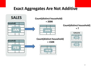
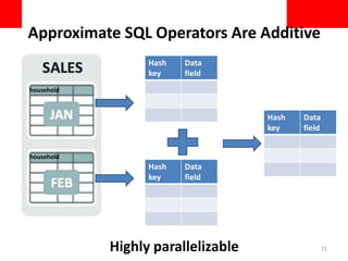
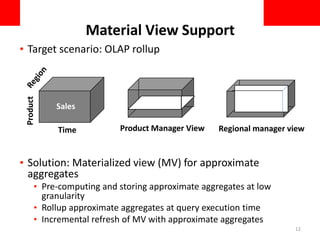
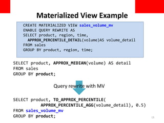
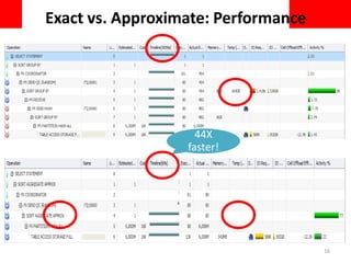
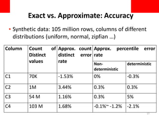
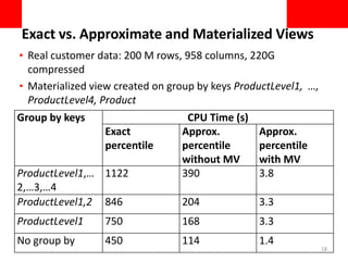
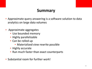
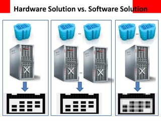
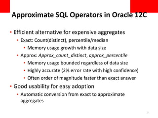
Copyright © 2016, Oracle and/or its affiliates. All rights reserved. |
Approximate Aggregates
In Oracle 12C
Hong Su, Mohamed Zait,
Vladimir Barrière, Joseph
Torres, Andre Menck
CIKM
Oct 27, 2016
Indianapolis
Challenges
• Larger data volume
• Traditional data sources: data
warehouse grows from tera
to peta bytes
• New data sources: Internet
Of Things (IOT), Internet of
cars...
• Stricter response time
requirements
• Real-time business
intelligence
• Visualization tools supporting
explorative/interactive
queries
• Traditional applications in
new pay-as-you-go cloud
infrastructure
2
Approximate Results Are Acceptable
• Visualization tools: Slightly inaccurate answers make no visual
difference
• Analytic queries: summary reports reveal patterns or trends
only
• Explorative queries: show low resolution answers before drill-
down
• Data science queries: early iterations of machine learning
queries tolerate approximation
3
4
Hardware Solution vs. Software Solution
…
… …
Approximate Query Solutions
5
Use summaries
(sketches, wavelets…)
Online aggregation
Use samples
Run more efficient
operator
Oracle 12C Solution
6
Use summaries
(sketches, wavelets…)
Online aggregation
Use samples
Run more efficient
operator
Approximate SQL Operators in Oracle 12C
• Efficient alternative for expensive aggregates
• Exact: Count(distinct), percentile/median
• Memory usage growth with data size
• Approx: Approx_count_distinct, approx_percentile
• Memory usage bounded regardless of data size
• Highly accurate (2% error rate with high confidence)
• Often order of magnitude faster than exact answer
• Good usability for easy adoption
• Automatic conversion from exact to approximate
aggregates
7
Approximate Count Distinct
• Based on Hyperloglog probabilistic counting
algorithm [FFG+07]
• Uses bounded memory (~4K bytes) per group by key
• Optimized to use smaller memory when group is small
• Significantly reduces chance to spill to disk
8
[FFG+07] Hyperloglog: the analysis of a near-optimal cardinality estimation
algorithm. Flajolet, Fusy, Gandouet and Meunier. Proceedings of the 2007
international conference on the analysis of algorithms.
SELECT APPROX_COUNT_DISTINCT(household),
APPROX_COUNT_DISTINCT(creditcard)
FROM sales
Group by region;
Approximate Percentile
• Offers both deterministic and non-deterministic alternatives
• Deterministic: Count-min sketch [C09]
• Results immune to data arrival order
• Non-deterministic: RANDOM [WLY+ 13]
• generally faster (default)
• Bounded memory (~8K bytes) per group by key – 2% error rate
with 95% confidence
9
[WLYC13] Quantiles over data streams: an experimental study, SIGMOD 2013
[C09] Count-min sketch. Cormode. Encyclopedia of database systems 2009
SELECT APPROX_MEDIAN(volume [DETERMINISTIC])
FROM sales
GROUP BY region;
Exact Aggregates Are Not Additive
10
household
household
Count(distinct household)
= 200K
Count(distinct household)
= 150K
Count(distinct household)
= ?
Approximate SQL Operators Are Additive
11
household
household
Highly parallelizable
Hash
key
Data
field
Hash
key
Data
field
Hash
key
Data
field
Material View Support
• Target scenario: OLAP rollup
• Solution: Materialized view (MV) for approximate
aggregates
• Pre-computing and storing approximate aggregates at low
granularity
• Rollup approximate aggregates at query execution time
• Incremental refresh of MV with approximate aggregates
Regional manager viewProduct Manager ViewTime
Product
Sales
12
Materialized View Example
CREATE MATERIALIZED VIEW sales_volume_mv
ENABLE QUERY REWRITE AS
SELECT product, region, time,
APPROX_PERCENTILE_DETAIL(volume)AS volume_detail
FROM sales
GROUP BY product, region, time;
SELECT product, APPROX_MEDIAN(volume) AS detail
FROM sales
GROUP BY product;
SELECT product, TO_APPROX_PERCENTILE(
APPROX_PERCENTILE_AGG(volume_detail), 0.5)
FROM sales_volume_mv
GROUP BY product;
Query rewrite with MV
13
Materialized View Example
SELECT region, APPROX_MEDIAN(volume) AS detail
FROM sales
GROUP BY region;
SELECT region, TO_APPROX_PERCENTILE(
APPROX_PERCENTILE_AGG(volume_detail), 0.5)
FROM sales_volume_mv
GROUP BY region; 14
CREATE MATERIALIZED VIEW sales_volume_mv
ENABLE QUERY REWRITE AS
SELECT product, region, time,
APPROX_PERCENTILE_DETAIL(volume)AS volume_detail
FROM sales
GROUP BY product, region, time;
Query Rewrite using MV
Experimental Results
15
44X
faster!
16
Exact vs. Approximate: Performance
Exact vs. Approximate: Accuracy
Column Count of
Distinct
values
Approx. count
distinct error
rate
Approx. percentile error
rate
Non-
deterministic
deterministic
C1 70K -1.53% 0% -0.3%
C2 1M 3.44% 0.3% 0.3%
C3 54 M 1.16% 0.3% 5%
C4 103 M 1.68% -0.1%~ -1.2% -2.1%
• Synthetic data: 105 million rows, columns of different
distributions (uniform, normal, zipfian …)
17
Exact vs. Approximate and Materialized Views
Group by keys CPU Time (s)
Exact
percentile
Approx.
percentile
without MV
Approx.
percentile
with MV
ProductLevel1,…
2,…3,…4
1122 390 3.8
ProductLevel1,2 846 204 3.3
ProductLevel1 750 168 3.3
No group by 450 114 1.4
• Real customer data: 200 M rows, 958 columns, 220G
compressed
• Materialized view created on group by keys ProductLevel1, …,
ProductLevel4, Product
18
Summary
• Approximate query answering is a software solution to data
analytics on large data volumes
• Approximate aggregates
• Use bounded memory
• Highly parallelizable
• Can be rolled up
• Materialized view rewrite possible
• Highly accurate
• Run much faster than exact counterparts
• Substantial room for further work!
19

cikm_2016_1027

  • 1.
    Copyright © 2016,Oracle and/or its affiliates. All rights reserved. | Approximate Aggregates In Oracle 12C Hong Su, Mohamed Zait, Vladimir Barrière, Joseph Torres, Andre Menck CIKM Oct 27, 2016 Indianapolis
  • 2.
    Challenges • Larger datavolume • Traditional data sources: data warehouse grows from tera to peta bytes • New data sources: Internet Of Things (IOT), Internet of cars... • Stricter response time requirements • Real-time business intelligence • Visualization tools supporting explorative/interactive queries • Traditional applications in new pay-as-you-go cloud infrastructure 2
  • 3.
    Approximate Results AreAcceptable • Visualization tools: Slightly inaccurate answers make no visual difference • Analytic queries: summary reports reveal patterns or trends only • Explorative queries: show low resolution answers before drill- down • Data science queries: early iterations of machine learning queries tolerate approximation 3
  • 4.
    4 Hardware Solution vs.Software Solution … … …
  • 5.
    Approximate Query Solutions 5 Usesummaries (sketches, wavelets…) Online aggregation Use samples Run more efficient operator
  • 6.
    Oracle 12C Solution 6 Usesummaries (sketches, wavelets…) Online aggregation Use samples Run more efficient operator
  • 7.
    Approximate SQL Operatorsin Oracle 12C • Efficient alternative for expensive aggregates • Exact: Count(distinct), percentile/median • Memory usage growth with data size • Approx: Approx_count_distinct, approx_percentile • Memory usage bounded regardless of data size • Highly accurate (2% error rate with high confidence) • Often order of magnitude faster than exact answer • Good usability for easy adoption • Automatic conversion from exact to approximate aggregates 7
  • 8.
    Approximate Count Distinct •Based on Hyperloglog probabilistic counting algorithm [FFG+07] • Uses bounded memory (~4K bytes) per group by key • Optimized to use smaller memory when group is small • Significantly reduces chance to spill to disk 8 [FFG+07] Hyperloglog: the analysis of a near-optimal cardinality estimation algorithm. Flajolet, Fusy, Gandouet and Meunier. Proceedings of the 2007 international conference on the analysis of algorithms. SELECT APPROX_COUNT_DISTINCT(household), APPROX_COUNT_DISTINCT(creditcard) FROM sales Group by region;
  • 9.
    Approximate Percentile • Offersboth deterministic and non-deterministic alternatives • Deterministic: Count-min sketch [C09] • Results immune to data arrival order • Non-deterministic: RANDOM [WLY+ 13] • generally faster (default) • Bounded memory (~8K bytes) per group by key – 2% error rate with 95% confidence 9 [WLYC13] Quantiles over data streams: an experimental study, SIGMOD 2013 [C09] Count-min sketch. Cormode. Encyclopedia of database systems 2009 SELECT APPROX_MEDIAN(volume [DETERMINISTIC]) FROM sales GROUP BY region;
  • 10.
    Exact Aggregates AreNot Additive 10 household household Count(distinct household) = 200K Count(distinct household) = 150K Count(distinct household) = ?
  • 11.
    Approximate SQL OperatorsAre Additive 11 household household Highly parallelizable Hash key Data field Hash key Data field Hash key Data field
  • 12.
    Material View Support •Target scenario: OLAP rollup • Solution: Materialized view (MV) for approximate aggregates • Pre-computing and storing approximate aggregates at low granularity • Rollup approximate aggregates at query execution time • Incremental refresh of MV with approximate aggregates Regional manager viewProduct Manager ViewTime Product Sales 12
  • 13.
    Materialized View Example CREATEMATERIALIZED VIEW sales_volume_mv ENABLE QUERY REWRITE AS SELECT product, region, time, APPROX_PERCENTILE_DETAIL(volume)AS volume_detail FROM sales GROUP BY product, region, time; SELECT product, APPROX_MEDIAN(volume) AS detail FROM sales GROUP BY product; SELECT product, TO_APPROX_PERCENTILE( APPROX_PERCENTILE_AGG(volume_detail), 0.5) FROM sales_volume_mv GROUP BY product; Query rewrite with MV 13
  • 14.
    Materialized View Example SELECTregion, APPROX_MEDIAN(volume) AS detail FROM sales GROUP BY region; SELECT region, TO_APPROX_PERCENTILE( APPROX_PERCENTILE_AGG(volume_detail), 0.5) FROM sales_volume_mv GROUP BY region; 14 CREATE MATERIALIZED VIEW sales_volume_mv ENABLE QUERY REWRITE AS SELECT product, region, time, APPROX_PERCENTILE_DETAIL(volume)AS volume_detail FROM sales GROUP BY product, region, time; Query Rewrite using MV
  • 15.
  • 16.
  • 17.
    Exact vs. Approximate:Accuracy Column Count of Distinct values Approx. count distinct error rate Approx. percentile error rate Non- deterministic deterministic C1 70K -1.53% 0% -0.3% C2 1M 3.44% 0.3% 0.3% C3 54 M 1.16% 0.3% 5% C4 103 M 1.68% -0.1%~ -1.2% -2.1% • Synthetic data: 105 million rows, columns of different distributions (uniform, normal, zipfian …) 17
  • 18.
    Exact vs. Approximateand Materialized Views Group by keys CPU Time (s) Exact percentile Approx. percentile without MV Approx. percentile with MV ProductLevel1,… 2,…3,…4 1122 390 3.8 ProductLevel1,2 846 204 3.3 ProductLevel1 750 168 3.3 No group by 450 114 1.4 • Real customer data: 200 M rows, 958 columns, 220G compressed • Materialized view created on group by keys ProductLevel1, …, ProductLevel4, Product 18
  • 19.
    Summary • Approximate queryanswering is a software solution to data analytics on large data volumes • Approximate aggregates • Use bounded memory • Highly parallelizable • Can be rolled up • Materialized view rewrite possible • Highly accurate • Run much faster than exact counterparts • Substantial room for further work! 19

Editor's Notes

  • #3 First of all, what are the challenges we are trying to address? The challenges have two aspects. First, the larger than ever data volume. Traditional data sources have been growing at an unprecedented rate. For example, ebay maintains a 90 peta byte data wharehouse about customer transactions and behaviors (8PB in teradta, 40PM in hadoop and 40P on custom system) as of 2013. On top of that, there are new data sources that can be even bigger than the traditional data sources because those data are machine generated such as those smart devices deplyed at your house. Imagine when driverless cars hit the market, we will have a surge of data coming from the internet of cars. The second aspect of the challenge is that the data analytics applications pose stricter response time requirements. For example, real-time business intelligence such as application performance monitoring, dynamic pricing or fraud detection all request immediate response instead of postmortem response. Visulatization tools allows user to issue explorative query or interactive queries. Even the traditional applications, when they are now deployed in the pay as you go cloud infrasture, have higher requirements on response time so as to reduce their payments. The combination of these two aspects make the problem harder. How do you answer queries faster on a larger data volume?
  • #4 Fortunately, we have observed in many of applications, approximate results are acceptable. For example, on visualization tools, slightly inaccurate answers make no visual difference. For analytic queries, summary reports care about patterns/trends. For example, if you know a certain website has a a million distinct user per month, that is good enough to make a business decision. It does not matter whether the actual number is 1.01 million. With this in mind, we can now seek a solution from a different angle.
  • #5 In the old days, you have configured your hardware based on your data size. Now there are many more times of data you have to process. You can throw in many more hardwares to get similar performance as before. You scale up or scale out the system. This is a hard ware solution. Instead, you can use the same hardware system but return approximate results as opposed to exact results. In other words, you trade the query quality for faster response time. Then we turn an expensive hardware solution into a much more economic software solution.
  • #6 Different categories of techniques can be used for approximate query processing. In the first category, people extract samples from the original data, run the query on the sample and extrapolate the results on the original data. In the second category, people create summary on the original data. Summary is usually a concise representation of the original data, such as sketches, histograms and wavelets. The third category is to provide more efficient operators. The same amount of input are consumed but the operators are efficient enough to provide results faster. The four category uses a completely different execution model called online aggregations. It produces the results as it reads the data. At the beginning the data processed is small,the results returned are associated with a large error rate. As more data are processed, the previous results are refined and the error rate decreases. If you let the query run to completion, then the results converge to exact results.
  • #7 So, what is our focus in our first release of approximate query features? We focus on providing more efficient aggregate operators. This fits into the existing database engine most easily among all the approaches.
  • #8 More specifically, we provide alternatives for expensive aggregates. count(distinct) and percentile are two commonly used aggregates. You can use count(distinct) to find distinct user or ip address of a website. You can use percentile to find outliers such as the value at 99 percentile or 1 percentile. Median is a special percentile. It is the value at 50 percentile. Both aggregates are expensive. Their memory consumption grows with number of distinct values or data size. When the data can no longer fit into the memory, it has to spill to disk. If disk spilling happens very often, the performance can take a huge hit. In contrast, the approximate alternatives uses bounded memory regardless of the data size.
  • #9 Now we will show you the syntax and the prominent features of these approximate aggregates. This is an example of how to use approx_count_distinct. It appears in any place that accepts count distinct except in the window function. This is a simple version. You can have multiple tables in the from clause and any other complicated constructs. The approx count distinct is based on state of the art hyperloglog probabilistic counting algorithm. Each aggregate operator uses about 4k memory per group by key. The core structure is a hash table. We ran experiments on various data types and found that 4k is a good setting. It achieves a reasonably low error rate about 2%. Settings higher than 4k do not give much observable accuracy improvement. When the group size is small, for example, if the number of rows falling into a certain region is small, we further optimize it so that the memory usage can be even smaller than 4K. Since we use such small memory, we significantly reduce chance to spill to disk. We also relieve the pressure on system memory resource so that the system can run far more queries at the same time.
  • #10 NOTE Now let’s see how we use approximate percentile. This query returns the median sales volume per region. A prominent feature of approximate percentile is that we provide two versions of it. One is deterministc and the other one is non-deterministic. The deterministic version guarantees to return exactly the same results from run to run, regardless how the data arrival order or whether you execute the query in serial or in parallel. Non-deterministic is generally faster and is the default mode. Deterministic version is often 2 times slower than the non-deterministic version. User will have to decide which version fits their requirement best. For example, in this query, deterministic key word is optional.
  • #11 Besides bounded memory usage, approximate aggregates also have an very important property. That is, they are additive. What does that mean? Let’s look at the example. Let’s say, we have a sales table which is divided into two parts, one part storing the sales data for january and the othe part storing the sales data for February. You apply count distinct on Jan’s data and get that there are 200K distinct household that had made purchase. Similarly, you apply count distinct on Feb’s data and get that there are 150K distinct household. Then what is the number of distinct household in total? You can’t tell except that the number can fall anywhere between 150K and 350K. We such such aggregates are not additive.
  • #12 In contrast, approximate sql operators are additive. As we have mentioned, the core data structure of the approx_count_distint function is a hash table. Approx_count_distinct_detail function will return this hash table. You can apply approx_count_distinct_detail function on jan’s data and get a hash table. Again you apply the same funciton on Feb’s data and get a second hash table. You merge these two hash tables and get one hash table. The hash table is the same as the one you will get if you directly apply approx_count_distinct_detail funciton on the sales table. Then you can derive approx count distinct from the final hash table. This is a key property. This makes the approximate aggregates highly parallelizable. You can process different parts of the data at the same time and merge them in the final phase.
  • #13 The additive property also makes an important feature materialized view possible. This is mainly used in OLAP environment. In OLAp applications, users can often request data at different dimensions. For example your sales table can have three major dimensions. It has information about when the sales is made, what product has been sold and where it is sold. A product manager view will care about the sales volume per product while a regional manager cares about the sales volume per region. In such case materialized views are very valuable. It will precompute and store approximate aggregates at lower graunlarity. It then rollup approximate aggregates to the higher granularity at query execution time.
  • #14 You aggregate the approximate percentile internal structure that belong to the same product. Then on top of that, you apply a scalar function to get the value at 50% percentile from the internal structure.
  • #15 Now a different query is issued by the region manager. He asks for the median sales volume per region. The query is different but you can still use the same materialized view. This time you aggregate all the internal structures that belong to the same region together. Because of the additive feature, the materialized view can be also refreshed incrementally. Meaning when data have changed, you don’t have to create the materialized view from scratch. Instead you can compute the approximate percentile internal structure on the delta changes and then combine the delta internal structure with the existing delta internal structure.
  • #17 Three stage plans if having multiple count(distinct ) .lower stage: partial duplicate eliminate (PIV) . intermediate stage: final duplicate eliminate (TIV) . final stage: aggregation (CIV) The first experiment showcases the performance gains of approximate aggregates over exact. The query has two count distinct
  • #18 We test a variety of columns with different distributions.