Chapter 2_System Modeling using computer(1).pptx

System Modeling
Identification
Lecturer: VU VAN PHONG
Dr. Van-Phong Vu-Department of Automatic Control

Textbook and References
 [1] Bài gi ng Mô hình hóa và nh n d ng h th ng
ả ậ ạ ệ ố , PGS. TS. Huỳnh Thái
Hoàng, ĐHQG TPHCM.
 [2] Giáo trình mô hình hóa và mô ph ng
ỏ , PGS. TS. Quy n Huy Ánh,
ề
ĐHSPKT 2010.
 [3] D. L. Smith, Introduction to Dynamic Systems Modeling for Design,
Prentice-Hall, 1994.
 [4] L. Ljung, System Identification – Theory for the users, 2nd
Edition,
Prentice-Hall, 1999.
 [5] R. Johansson, System Modeling and Identification, Prentice-Hall,
1993.
 [6] L. Ljung, System Identification ToolboxTM
Getting Started Guide in
Matlab, The MathWorks, Inc, 2016

Contents of This course
 Chapter 1: Introduction
 Chapter 2: System Modeling
 Chapter 3: Non-parameter System Identification
 Chapter 4: Structure of the Parameter System
 Chapter 5: Parameter Estimation System Identification
 Chapter 6: Evaluation model
 Chapter 7: System Identification in Practice

Chapter 2: System Modeling

Contents of Chapter 2
 2.1 Introduction
 2.2 Functional Analysis
 2.3 Physical Characteristic Analysis
2.3.1 Modeling a Mechanical System
2.3.2 Modeling an Electrical System
2.3.3 Modeling of Electromechanical Systems
2.3.4 Modeling of Fluid Systems
2.3.5 Modeling of Thermal Systems
 2.4 Mathematical Model Analysis

2.1 Introduction
 System Modeling: procedure to build the mathematical
model of the system based on the physical laws of the
system

2.1 Introduction
System Modeling
Functional
Analysis
Physical
Characteristic
Analysis
Mathematical
Model Analysis

2.2 Functional Analysis

2.2 Function Analysis of the System
 Functional analysis: analyze the system into a set of
subsystems which consist of the functional components.
 During functional analysis, we need to note the
Connectivity: which parts of the system connect together.
Causality: How the parts of the system connect?

2.2 Functional Analysis of the System
 Procedure for Functional Analysis:
Step 1: Isolate the system with environment.
Step 2: Analyze the subsystems
Step 3: Determine the causality

 Isolate the system with environment:
Determine the limited area of the system.
Cut off all connections between the system with outside
environment.
Replace each connection by a port to describe the
interactions between system and environment.

 Ports: are the terminals (thi t b đ u cu i) of the system in
ế ị ầ ố
which the energy is transferred in or out. The system can
have single or multiple ports.
 One port can have one/two inputs (U) one/two ouput
(Y).
 Common ports:
Structural (c khí)
ơ
Electrical (Đi n)
ệ
Thermal (Nhi t)
ệ
Fluid (L u ch t)
ư ấ

 Structural

 Electrical

 Thermal

 Fluid

 Example:

 Example: Cooling system

 Subsystem Analysis:
Divide the system into subsystems
Divide the subsystems into components.
Replace the connectivity among components by
ports.

 Subsystem Analysis:

 Determine Causality:
 Causality is determined by the variables at the ports.

2.3 Physical Characteristic
Analysis

 Physical Characteristic Analysis: a process to obtain the
mathematical model of each functional component based
on the physical laws.
 Basic physical systems:
Electrical system
Mechanical System
Thermal system
Fluid system
2.3 Physical Characteristic Analysis


Physical systems
Basic Elements Basic Variables Conservation laws
1. Resistance
2. Capacitance
3. Inductance/
Inertia
1. Quantity
2. Potentiality
3. Time
Electrical,
Mechanical,
Thermal,
Fluid

 Mechanical System:
 Basic Variables:
Distance (quantity) x [m]
Force (potentiality) F [N]
Velocity v [m/s]
 Basic elements:
Dashpot ( Piston cylinder):
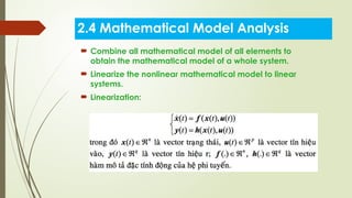
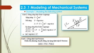
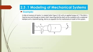
2.3 .1 Modeling of Mechanical Systems
𝑓 =𝑏
𝑑𝑥
𝑑𝑡
=𝑏𝑣

Spring.
Mass:
Energy : 𝐸=
1
2
𝑘 𝑥
2
Newton law 2:
𝑓 =𝑚𝑎=𝑚
𝑑𝑣
𝑑𝑡
=𝑚
𝑑2
𝑥
𝑑𝑡
2 𝐸=
1
2
𝑚𝑣
2
Energy:

 Conservation Laws:
Force equilibrium equations, Newton Laws.
Euler-Lagrange Equations

 Example 1: Modeling the following system

 Example 2:
m
F1=kX(t)
Fms=bv(t)
F(t)
b
F: Force
X(t): Displacement
v: velocity
m: mass
K: spring constant
b: Damping coefficient

 Example 3:

 Example 3: Modeling the following system

 Example 4: Modeling the train

 Example 3: Modeling the train

 Consider a system illustrated in Fig. 6. and are the external force (inputs) ;
and and are the displacement of m1 and m2, respectively.
 Please determine the mathematical model in term of state-space
equation.
 Please simulate the system using Matlab/Simulink
 with inputs are step signal m1=1, m2=2 b=0.1, k1=0.15, k2=0.15

 Rotational Mechanical Systems : The input to a rotational
mechanical system may be the torque T and the output
the rotational displacement, or angle.
Torsional spring: relationship between torque T and the
angle θ rotated by the spring

 Rotational Mechanical Systems :
 Rotational dashpot:
 Moment of inertia: torque T, angular acceleration a, and
the moment of inertia I,


 Example:

Electrical System:
Basic variables:
Charge (đi n l ng) q [C]
ệ ượ
Voltage (đi n th ) u [V]
ệ ế
Current ( dòng đi n) I [A]
ệ
Basic elements
Resistance: Capacitance:
Inductance:
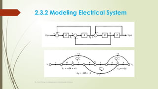
2.3.2 Modeling Electrical System

Conservation Laws:
v21 L
t
i
d
d
 E
1
2
L
 i
2

i C
t
v21
d
d
 E
1
2
M
 v21
2

Kirchhoff’s voltage law

Conservation Laws:
Kirchoff Law for current
Kirchoff law for voltage
 Analysis circuit methods

 Example 1:
C
C
C
C
v
dt
v
d
LC
dt
dv
RC
v
dt
di
L
R
i
v






2
2
.

 Example 2:

2.3.3 Modeling of Electromechanical Systems
 Transfer function of DC motor
T w
U
R
J
+
L
Kf
-
i
Lư
Rư
Uư
Eư

Mt
B
J
Điện cảm phần ứng
Điện trở phần ứng
Điện áp phần ứng
Sức điện động phần ứng
Tốc độ động cơ
Mô men tải
Hệ số ma sát
Mô men quán tính

 Ph ng trình cân b ng đi n
ươ ằ ệ

)
(
)
(
)
(
)
(
.
).
(
)
(
u
t
K
t
E
t
E
dt
t
di
L
R
t
i
t
U
u
u
u
u
u
u






 Ph ng trình cân b ng moment
ươ ằ

)
(
)
(
)
(
)
(
)
(
)
(
t
i
K
t
M
dt
t
d
J
t
B
t
M
t
M
u
đ
t
đ








Fluid Systems:
Basic variables:
Pressure (áp su t) p [N/m
ấ 2
]
Volume (th tích) V [m
ể 3
]
Flow ( l u l ng) z [m
ư ượ 3
/s]
Basic elements
Hydraulic resistance
2.3.4 Modeling the Fluid Systems

Fluid Systems:
Hydraulic resistance R:

Fluid Systems:
Hydraulic Capacitance C:
(1)
(2)
Hydraulic Capacitance C

Fluid Systems:
Hydraulic inertance: Hydraulic capacitance is a measure of
the energy storage in a hydraulic system.
P1 − P2 be the pressure drop
cross-sectional area A
 m is the uid mass and
v is the fluid velocity
 pipe length is L
Newton’s second law

 Example:
L

 Thermal Systems:
Thermal resistance R is the resistance offered to the
heat flow

2.3.5 Modeling of Thermal System

 Thermal Systems:
Thermal capacitance is a measure of the energy
storage in a thermal system
 q1 is the heat flowing into a body
q2 is the heat owing out
the difference q2 − q1 is stored by the body
heat capacity be denoted by C

Example:

2.4 Mathematical Model
Analysis

2.4 Mathematical Model Analysis
 Combine all mathematical model of all elements to
obtain the mathematical model of a whole system.
 Linearize the nonlinear mathematical model to linear
systems.
 Linearization:

 Equilibrium point (Đi m d ng).
ể ừ

 How to find Equilibrium point

Thank You For Your Listening

Chapter 2_System Modeling using computer(1).pptx

More Related Content

Similar to Chapter 2_System Modeling using computer(1).pptx

Recently uploaded

Chapter 2_System Modeling using computer(1).pptx