More Related Content

PPTX
Discriminant Analysis.pptx 
PPTX
Discriminant analysis-Business Intelligence tool 
PPTX
Discriminant analysis and its applications in business decision.pptx 
PPT
T18 discriminant analysis 
PPTX
Discriminant analysis.pptx 
PDF

PPT

PDF
Discrimination Analysis and working on SPSS assignment Similar to Chapter 07 _discriminant + logistihjc.ppt

PPTX
Discriminate Analysis for health statistics .pptx 
PPTX
DISCRIMINANT ANALYSIS.pptx 
PPTX
discriminantfunctionanalysisdfa-200926121304(1).pptx 
PPTX
discriminantfunctionanalysisdfa-200926121304.pptx 
PPTX
discriminate analysis of Biostatistics ppt for MPH Students 
PPTX

PPTX
Discriminant function analysis (DFA) 
PPTX

PPT
Discriminant analysis group no. 4 
PPTX
DISCRIMINABLE CLUSTER ANALYSIS.pptx 
PPTX

PDF
Use of Discriminant Analysis in Research 
PPTX
Discriminant Analysis in Sports 
PPTX

PPT

PPTX

PPT
Discriminant analysis tehnik analisa Statistika Chap11.ppt 
PDF
An Overview and Application of Discriminant Analysis in Data Analysis 
PPT

PPTX
diiscriminant analysis1.pptx Recently uploaded

PPTX
Lecture 8 Standardisation vs Adaptation - International Product Management A... 
PPTX
Local AEO Best Practices for Small Businesses in 2026 
DOCX
Visit usasmmpoint Buy Linkedin account -2013-2026 -pva 
PPTX
The State of AEO & GEO in 2026: Forecast, Investments, & Strategies 
PDF
Buy Hotmail Accounts in Bulk Safely_ 100% Verified and Aged Alternative.pdf 
DOCX
Buying Reddit Karma Accounts in 2026 - A Detailed Guide.docx 
PDF
2025 State of Marketing Report – by Hubspot 
DOCX
The Process of Purchase Old Facebook Accounts From 2015 to 2026.docx 
PDF
An Influencer Marketing Agency in India Built for Results 
PDF
Neil Isler on Crafting a Winning Marketing Strategy for Your Startup 
PPTX
LESSON 1 INTRODUCTION TO PURCHASING AND PRICING STRATEGY.pptx 
PPTX
Salt Lake City Marketo User Group - New Year New You-ser Group (Adding AI to ... 
DOCX
Best Web to Learn About Buying Verified PayPal Accounts (Los Angeles).docx ![[EN].CleverGroup Vietnam Profile 20251202](https://cdn.slidesharecdn.com/ss_thumbnails/en-260120091417-fe6f88ec-thumbnail.jpg?width=640&height=640&fit=bounds)
PDF
[EN].CleverGroup Vietnam Profile 20251202 
PDF
Top 7 Websites List Buy Gmail Accounts ( PVA, OLD & AGED ). 
PDF
Digital Marketing Strategist | Lubna.P.S 
PDF
Philippines Ceramic Tiles Market Size, Share & Trends 
PDF
Pet Care SEO Strategy: How Pet Businesses Can Rank Higher & Get More Clients 
PPTX
This is a presentation about Website Designing 
PDF
Prashant Gorhe - Digital Marketing - Portfolio Chapter 07 _discriminant + logistihjc.ppt
- 1.
Copyright © 2010Pearson Education, Inc., publishing as Prentice-Hall. 5-1
Chapter 7
Chapter 7
Multiple Discriminant Analysis
Multiple Discriminant Analysis
and Logistic Regression
and Logistic Regression
- 2.
Copyright © 2010Pearson Education, Inc., publishing as Prentice-Hall. 5-2
LEARNING OBJECTIVES
LEARNING OBJECTIVES
Upon completing this chapter, you should be able to
Upon completing this chapter, you should be able to
do the following:
do the following:
• State the circumstances under which a linear
State the circumstances under which a linear
discriminant analysis should be used instead of
discriminant analysis should be used instead of
multiple regression.
multiple regression.
• Identify the major issues relating to types of
Identify the major issues relating to types of
variables used and sample size required in the
variables used and sample size required in the
application of discriminant analysis.
application of discriminant analysis.
• Understand the assumptions underlying
Understand the assumptions underlying
discriminant analysis in assessing its
discriminant analysis in assessing its
appropriateness for a particular problem.
appropriateness for a particular problem.
Chapter 7
Chapter 7
Multiple Discriminant Analysis
Multiple Discriminant Analysis
and Logistic Regression
and Logistic Regression
- 3.
Copyright © 2010Pearson Education, Inc., publishing as Prentice-Hall. 5-3
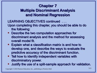
LEARNING OBJECTIVES continued . . .
LEARNING OBJECTIVES continued . . .
Upon completing this chapter, you should be able to do
Upon completing this chapter, you should be able to do
the following:
the following:
• Describe the two computation approaches for
Describe the two computation approaches for
discriminant analysis and the method for assessing
discriminant analysis and the method for assessing
overall model fit.
overall model fit.
• Explain what a classification matrix is and how to
Explain what a classification matrix is and how to
develop one, and describe the ways to evaluate the
develop one, and describe the ways to evaluate the
predictive accuracy of the discriminant function.
predictive accuracy of the discriminant function.
• Tell how to identify independent variables with
Tell how to identify independent variables with
discriminatory power.
discriminatory power.
• Justify the use of a split-sample approach for validation.
Justify the use of a split-sample approach for validation.
Chapter 7
Chapter 7
Multiple Discriminant Analysis
Multiple Discriminant Analysis
and Nominal Regression
and Nominal Regression
- 4.
Copyright © 2010Pearson Education, Inc., publishing as Prentice-Hall. 5-4
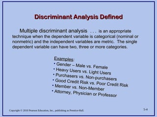
Multiple discriminant analysis
Multiple discriminant analysis . . . is an appropriate
. . . is an appropriate
technique when the dependent variable is categorical (nominal or
technique when the dependent variable is categorical (nominal or
nonmetric) and the independent variables are metric. The single
nonmetric) and the independent variables are metric. The single
dependent variable can have two, three or more categories.
dependent variable can have two, three or more categories.
Discriminant Analysis Defined
Discriminant Analysis Defined
Examples
Examples:
:
• Gender – Male vs. Female
Gender – Male vs. Female
• Heavy Users vs. Light Users
Heavy Users vs. Light Users
• Purchasers vs. Non-purchasers
Purchasers vs. Non-purchasers
• Good Credit Risk vs. Poor Credit Risk
Good Credit Risk vs. Poor Credit Risk
• Member vs. Non-Member
Member vs. Non-Member
• Attorney, Physician or Professor
Attorney, Physician or Professor
- 5.
Copyright © 2010Pearson Education, Inc., publishing as Prentice-Hall. 5-5
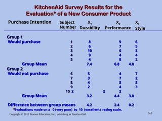
KitchenAid Survey Results for the
KitchenAid Survey Results for the
Evaluation* of a New Consumer Product
Evaluation* of a New Consumer Product
X
X3
3
Style
Style
Group 1
Group 1
Would purchase
Would purchase 1
1 8
8 9
9 6
6
2
2 6
6 7
7 5
5
3
3 10
10 6
6 3
3
4
4 9
9 4
4 4
4
5
5 4
4 8
8 2
2
Group Mean
Group Mean 7.4
7.4 6.8 4.0
6.8 4.0
Group 2
Group 2
Would not purchase
Would not purchase 6
6 5
5 4
4 7
7
7
7 3
3 7
7 2
2
8
8 4
4 5
5 5
5
9
9 2
2 4
4 3
3
10
10 2
2 2
2 2
2
Group Mean
Group Mean 3.2
3.2 4.4 3.8
4.4 3.8
Difference between group means
Difference between group means 4.2
4.2 2.4 0.2
2.4 0.2
Purchase Intention
Purchase Intention Subject
Subject
Number
Number
X
X1
1
Durability
Durability
X
X2
2
Performance
Performance
*
*Evaluations made on a 0 (very poor) to 10 (excellent) rating scale.
Evaluations made on a 0 (very poor) to 10 (excellent) rating scale.
- 6.
Copyright © 2010Pearson Education, Inc., publishing as Prentice-Hall. 5-6
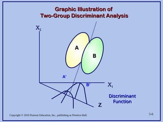
Graphic Illustration of
Graphic Illustration of
Two-Group Discriminant Analysis
Two-Group Discriminant Analysis
X
X2
2
X
X1
1
Z
Z
Discriminant
Discriminant
Function
Function
A’
B’
A
B
- 7.
Copyright © 2010Pearson Education, Inc., publishing as Prentice-Hall. 5-7
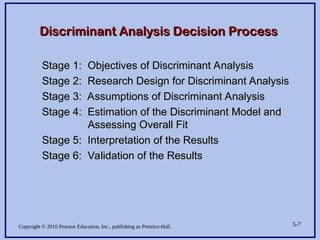
Discriminant Analysis Decision Process
Discriminant Analysis Decision Process
Stage 1: Objectives of Discriminant Analysis
Stage 1: Objectives of Discriminant Analysis
Stage 2: Research Design for Discriminant Analysis
Stage 2: Research Design for Discriminant Analysis
Stage 3: Assumptions of Discriminant Analysis
Stage 3: Assumptions of Discriminant Analysis
Stage 4: Estimation of the Discriminant Model and
Stage 4: Estimation of the Discriminant Model and
Assessing Overall Fit
Assessing Overall Fit
Stage 5: Interpretation of the Results
Stage 5: Interpretation of the Results
Stage 6: Validation of the Results
Stage 6: Validation of the Results
- 8.
Copyright © 2010Pearson Education, Inc., publishing as Prentice-Hall. 5-8
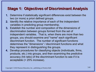
Stage 1: Objectives of Discriminant Analysis
Stage 1: Objectives of Discriminant Analysis
1.
1. Determine if statistically significant differences exist between the
Determine if statistically significant differences exist between the
two (or more) a priori defined groups.
two (or more) a priori defined groups.
2.
2. Identify the relative importance of each of the independent
Identify the relative importance of each of the independent
variables in predicting group membership.
variables in predicting group membership.
3.
3. Establish the number and composition of the dimensions of
Establish the number and composition of the dimensions of
discrimination between groups formed from the set of
discrimination between groups formed from the set of
independent variables. That is, when there are more than two
independent variables. That is, when there are more than two
groups, you should examine and "name" each significant
groups, you should examine and "name" each significant
discriminant function. The number of significant functions
discriminant function. The number of significant functions
determines the "dimensions“ / discriminant functions and what
determines the "dimensions“ / discriminant functions and what
they represent in distinguishing the groups.
they represent in distinguishing the groups.
4.
4. Develop procedures for classifying objects (individuals, firms,
Develop procedures for classifying objects (individuals, firms,
products, etc.) into groups, and then examining the predictive
products, etc.) into groups, and then examining the predictive
accuracy (hit ratio) of the discriminant function to see if it is
accuracy (hit ratio) of the discriminant function to see if it is
acceptable (> 25% increase).
acceptable (> 25% increase).
- 9.
Copyright © 2010Pearson Education, Inc., publishing as Prentice-Hall. 5-9
• Selection of dependent and
Selection of dependent and
independent variables.
independent variables.
• Sample size (total & per variable).
Sample size (total & per variable).
• Sample division for validation.
Sample division for validation.
Stage 2: Research Design for Discriminant Analysis
Stage 2: Research Design for Discriminant Analysis
- 10.
Copyright © 2010Pearson Education, Inc., publishing as Prentice-Hall. 5-10
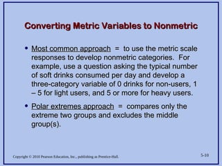
Converting Metric Variables to Nonmetric
Converting Metric Variables to Nonmetric
• Most common approach
Most common approach = to use the metric scale
= to use the metric scale
responses to develop nonmetric categories. For
responses to develop nonmetric categories. For
example, use a question asking the typical number
example, use a question asking the typical number
of soft drinks consumed per day and develop a
of soft drinks consumed per day and develop a
three-category variable of 0 drinks for non-users, 1
three-category variable of 0 drinks for non-users, 1
– 5 for light users, and 5 or more for heavy users.
– 5 for light users, and 5 or more for heavy users.
• Polar extremes approach
Polar extremes approach = compares only the
= compares only the
extreme two groups and excludes the middle
extreme two groups and excludes the middle
group(s).
group(s).
- 11.
Copyright © 2010Pearson Education, Inc., publishing as Prentice-Hall. 5-11
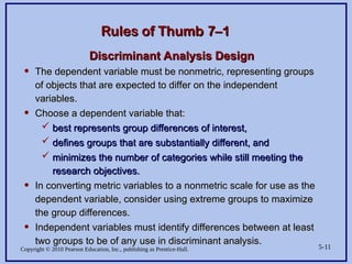
Rules of Thumb 7–1
Rules of Thumb 7–1
Discriminant Analysis Design
Discriminant Analysis Design
• The dependent variable must be nonmetric, representing groups
The dependent variable must be nonmetric, representing groups
of objects that are expected to differ on the independent
of objects that are expected to differ on the independent
variables.
variables.
• Choose a dependent variable that:
Choose a dependent variable that:
best represents group differences of interest,
best represents group differences of interest,
defines groups that are substantially different, and
defines groups that are substantially different, and
minimizes the number of categories while still meeting the
minimizes the number of categories while still meeting the
research objectives.
research objectives.
• In converting metric variables to a nonmetric scale for use as the
In converting metric variables to a nonmetric scale for use as the
dependent variable, consider using extreme groups to maximize
dependent variable, consider using extreme groups to maximize
the group differences.
the group differences.
• Independent variables must identify differences between at least
Independent variables must identify differences between at least
two groups to be of any use in discriminant analysis.
two groups to be of any use in discriminant analysis.
- 12.
Copyright © 2010Pearson Education, Inc., publishing as Prentice-Hall. 5-12
Rules of Thumb 7–1 continued . . .
Rules of Thumb 7–1 continued . . .
• The sample size must be large enough to:
The sample size must be large enough to:
have at least one more observation per group than the number of
have at least one more observation per group than the number of
independent variables, but striving for at least 20 cases per group.
independent variables, but striving for at least 20 cases per group.
have 20 cases per independent variable, with a minimum
have 20 cases per independent variable, with a minimum
recommended level of 5 observations per variable.
recommended level of 5 observations per variable.
have at least one more observation per group than the number of
have at least one more observation per group than the number of
independent variables, but striving for at least 20 cases per group.
independent variables, but striving for at least 20 cases per group.
have a large enough sample to divide it into an estimation and holdout
have a large enough sample to divide it into an estimation and holdout
sample, each meeting the above requirements.
sample, each meeting the above requirements.
• Assess the equality of covariance matrices with the Box’s M test, but apply
Assess the equality of covariance matrices with the Box’s M test, but apply
a conservative significance level of .01.
a conservative significance level of .01.
• Examine the independent variables for univariate normality.
Examine the independent variables for univariate normality.
• Multicollinearity among the independent variables can markedly reduce the
Multicollinearity among the independent variables can markedly reduce the
estimated impact of independent variables in the derived discriminant
estimated impact of independent variables in the derived discriminant
function(s), particularly if a stepwise estimation process is used.
function(s), particularly if a stepwise estimation process is used.
- 13.
Copyright © 2010Pearson Education, Inc., publishing as Prentice-Hall. 5-13
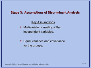
Stage 3: Assumptions of Discriminant Analysis
Stage 3: Assumptions of Discriminant Analysis
Key Assumptions
Key Assumptions
• Multivariate normality of the
Multivariate normality of the
independent variables.
independent variables.
• Equal variance and covariance
Equal variance and covariance
for the groups.
for the groups.
- 14.
Copyright © 2010Pearson Education, Inc., publishing as Prentice-Hall. 5-14
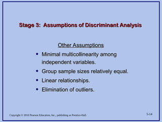
Other Assumptions
Other Assumptions
• Minimal multicollinearity among
Minimal multicollinearity among
independent variables.
independent variables.
• Group sample sizes relatively equal.
Group sample sizes relatively equal.
• Linear relationships.
Linear relationships.
• Elimination of outliers.
Elimination of outliers.
Stage 3: Assumptions of Discriminant Analysis
Stage 3: Assumptions of Discriminant Analysis
- 15.
Copyright © 2010Pearson Education, Inc., publishing as Prentice-Hall. 5-15
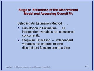
Stage 4: Estimation of the Discriminant
Stage 4: Estimation of the Discriminant
Model and Assessing Overall Fit
Model and Assessing Overall Fit
Selecting An Estimation Method . . .
Selecting An Estimation Method . . .
1.
1. Simultaneous Estimation – all
Simultaneous Estimation – all
independent variables are considered
independent variables are considered
concurrently.
concurrently.
2.
2. Stepwise Estimation – independent
Stepwise Estimation – independent
variables are entered into the
variables are entered into the
discriminant function one at a time
discriminant function one at a time.
.
- 16.
Copyright © 2010Pearson Education, Inc., publishing as Prentice-Hall. 5-16
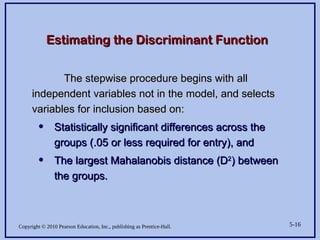
Estimating the Discriminant Function
Estimating the Discriminant Function
The stepwise procedure begins with all
The stepwise procedure begins with all
independent variables not in the model, and selects
independent variables not in the model, and selects
variables for inclusion based on:
variables for inclusion based on:
• Statistically significant differences across the
Statistically significant differences across the
groups (.05 or less required for entry), and
groups (.05 or less required for entry), and
• The largest Mahalanobis distance (D
The largest Mahalanobis distance (D2
2
) between
) between
the groups.
the groups.
- 17.
Copyright © 2010Pearson Education, Inc., publishing as Prentice-Hall. 5-17
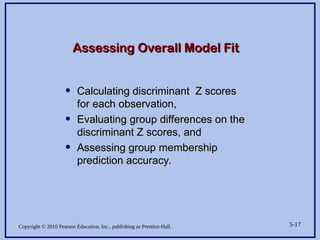
Assessing Overall Model Fit
Assessing Overall Model Fit
• Calculating discriminant Z scores
Calculating discriminant Z scores
for each observation,
for each observation,
• Evaluating group differences on the
Evaluating group differences on the
discriminant Z scores, and
discriminant Z scores, and
• Assessing group membership
Assessing group membership
prediction accuracy.
prediction accuracy.
- 18.
Copyright © 2010Pearson Education, Inc., publishing as Prentice-Hall. 5-18
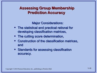
Assessing Group Membership
Assessing Group Membership
Prediction Accuracy
Prediction Accuracy
Major Considerations:
Major Considerations:
• The statistical and practical rational for
The statistical and practical rational for
developing classification matrices,
developing classification matrices,
• The cutting score determination,
The cutting score determination,
• Construction of the classification matrices,
Construction of the classification matrices,
and
and
• Standards for assessing classification
Standards for assessing classification
accuracy.
accuracy.
- 19.
Copyright © 2010Pearson Education, Inc., publishing as Prentice-Hall. 5-19
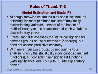
Rules of Thumb 7–2
Rules of Thumb 7–2
Model Estimation and Model Fit
Model Estimation and Model Fit
• Although stepwise estimation may seem “optimal” by
Although stepwise estimation may seem “optimal” by
selecting the most parsimonious set of maximally
selecting the most parsimonious set of maximally
discriminating variables, beware of the impact of
discriminating variables, beware of the impact of
multicollinearity on the assessment of each variable’s
multicollinearity on the assessment of each variable’s
discriminatory power.
discriminatory power.
• Overall model fit assesses the statistical significance
Overall model fit assesses the statistical significance
between groups on the discriminant Z score(s), but
between groups on the discriminant Z score(s), but
does not assess predictive accuracy.
does not assess predictive accuracy.
• With more than two groups, do not confine your
With more than two groups, do not confine your
analysis to only the statistically significant discriminant
analysis to only the statistically significant discriminant
function(s), but consider if nonsignificant functions
function(s), but consider if nonsignificant functions
(with significance levels of up to .3) add explanatory
(with significance levels of up to .3) add explanatory
power.
power.
- 20.
Copyright © 2010Pearson Education, Inc., publishing as Prentice-Hall. 5-20
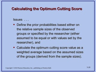
Calculating the Optimum Cutting Score
Calculating the Optimum Cutting Score
Issues . . .
Issues . . .
• Define the prior probabilities based either on
Define the prior probabilities based either on
the relative sample sizes of the observed
the relative sample sizes of the observed
groups or specified by the researcher (either
groups or specified by the researcher (either
assumed to be equal or with values set by the
assumed to be equal or with values set by the
researcher), and
researcher), and
• Calculate the optimum cutting score value as a
Calculate the optimum cutting score value as a
weighted average based on the assumed sizes
weighted average based on the assumed sizes
of the groups (derived from the sample sizes).
of the groups (derived from the sample sizes).
- 21.
Copyright © 2010Pearson Education, Inc., publishing as Prentice-Hall. 5-21
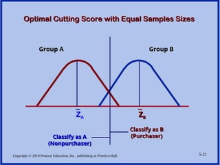
Optimal Cutting Score with Equal Samples Sizes
Optimal Cutting Score with Equal Samples Sizes
Group B
Group B
Group A
Group A
_
ZA
_
Z
ZB
B
Classify as B
Classify as B
(Purchaser)
(Purchaser)
Classify as A
Classify as A
(Nonpurchaser)
(Nonpurchaser)
- 22.
Copyright © 2010Pearson Education, Inc., publishing as Prentice-Hall. 5-22
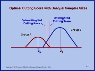
Optimal Cutting Score with Unequal Samples Sizes
Optimal Cutting Score with Unequal Samples Sizes
Group B
Group B
Group A
Group A
_
Z
ZA
A
_
Z
ZB
B
Optimal Weighted
Optimal Weighted
Cutting
Cutting Score
Score
Unweighted
Unweighted
Cutting Score
Cutting Score
- 23.
Copyright © 2010Pearson Education, Inc., publishing as Prentice-Hall. 5-23
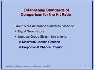
Establishing Standards of
Establishing Standards of
Comparison for the Hit Ratio
Comparison for the Hit Ratio
Group sizes determine standards based on:
Group sizes determine standards based on:
• Equal Group Sizes
Equal Group Sizes
• Unequal Group Sizes – two criteria:
Unequal Group Sizes – two criteria:
o Maximum Chance Criterion
Maximum Chance Criterion
o Proportional Chance Criterion
Proportional Chance Criterion
- 24.
Copyright © 2010Pearson Education, Inc., publishing as Prentice-Hall. 5-24
Classification Matrix
Classification Matrix
HBAT’s New Consumer Product
HBAT’s New Consumer Product
Actual
Actual
Group
Group
Would
Would
Purchase
Purchase
Would
Would
Not
Not
Purchase
Purchase
Actual
Actual
Total
Total
Percent
Percent
Correct
Correct
Classification
Classification
Predicted Group
Predicted Group
Percent Correctly Classified (hit ratio) =
Percent Correctly Classified (hit ratio) =
100 x [(22 + 20)/50] = 84%
100 x [(22 + 20)/50] = 84%
(1)
(1) 22
22 3
3 25
25
88%
88%
(2)
(2) 5
5 20
20 25
25
80%
80%
Predicted
Predicted
Total
Total
27
27 23
23 50
50
- 25.
Copyright © 2010Pearson Education, Inc., publishing as Prentice-Hall. 5-25
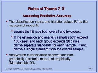
Rules of Thumb 7–3
Rules of Thumb 7–3
Assessing Predictive Accuracy
Assessing Predictive Accuracy
• The classification matrix and hit ratio replace R
The classification matrix and hit ratio replace R2
2
as the
as the
measure of model fit:
measure of model fit:
assess the hit ratio both overall and by group..
assess the hit ratio both overall and by group..
If the estimation and analysis samples both exceed
If the estimation and analysis samples both exceed
100 cases and each group exceeds 20 cases,
100 cases and each group exceeds 20 cases,
derive separate standards for each sample. If not,
derive separate standards for each sample. If not,
derive a single standard from the overall sample.
derive a single standard from the overall sample.
• Analyze the missclassified observations both
Analyze the missclassified observations both
graphically (territorial map) and empirically
graphically (territorial map) and empirically
(Mahalanobis D
(Mahalanobis D2
2
).
).
- 26.
Copyright © 2010Pearson Education, Inc., publishing as Prentice-Hall. 5-26
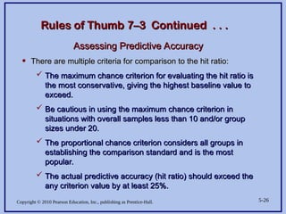
Rules of Thumb 7–3 Continued . . .
Rules of Thumb 7–3 Continued . . .
Assessing Predictive Accuracy
Assessing Predictive Accuracy
• There are multiple criteria for comparison to the hit ratio:
There are multiple criteria for comparison to the hit ratio:
The maximum chance criterion for evaluating the hit ratio is
The maximum chance criterion for evaluating the hit ratio is
the most conservative, giving the highest baseline value to
the most conservative, giving the highest baseline value to
exceed.
exceed.
Be cautious in using the maximum chance criterion in
Be cautious in using the maximum chance criterion in
situations with overall samples less than 10 and/or group
situations with overall samples less than 10 and/or group
sizes under 20.
sizes under 20.
The proportional chance criterion considers all groups in
The proportional chance criterion considers all groups in
establishing the comparison standard and is the most
establishing the comparison standard and is the most
popular.
popular.
The actual predictive accuracy (hit ratio) should exceed the
The actual predictive accuracy (hit ratio) should exceed the
any criterion value by at least 25%.
any criterion value by at least 25%.
- 27.
Copyright © 2010Pearson Education, Inc., publishing as Prentice-Hall. 5-27
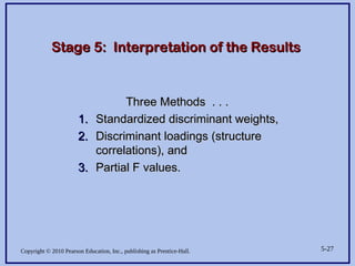
Stage 5: Interpretation of the Results
Stage 5: Interpretation of the Results
Three Methods . . .
Three Methods . . .
1.
1. Standardized discriminant weights,
Standardized discriminant weights,
2.
2. Discriminant loadings (structure
Discriminant loadings (structure
correlations), and
correlations), and
3.
3. Partial F values.
Partial F values.
- 28.
Copyright © 2010Pearson Education, Inc., publishing as Prentice-Hall. 5-28
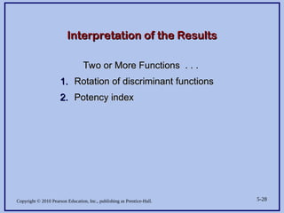
Interpretation of the Results
Interpretation of the Results
Two or More Functions . . .
Two or More Functions . . .
1.
1. Rotation of discriminant functions
Rotation of discriminant functions
2.
2. Potency index
Potency index
- 29.
Copyright © 2010Pearson Education, Inc., publishing as Prentice-Hall. 5-29
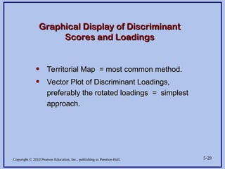
Graphical Display of Discriminant
Graphical Display of Discriminant
Scores and Loadings
Scores and Loadings
• Territorial Map = most common method.
Territorial Map = most common method.
• Vector Plot of Discriminant Loadings,
Vector Plot of Discriminant Loadings,
preferably the rotated loadings = simplest
preferably the rotated loadings = simplest
approach.
approach.
- 30.
Copyright © 2010Pearson Education, Inc., publishing as Prentice-Hall. 5-30
Plotting Procedure for Vectors
Plotting Procedure for Vectors
Three Steps . . .
Three Steps . . .
1.
1. Selecting variables,
Selecting variables,
2.
2. Stretching the vectors, and
Stretching the vectors, and
3.
3. Plotting the group centroids.
Plotting the group centroids.
- 31.
Copyright © 2010Pearson Education, Inc., publishing as Prentice-Hall. 5-31
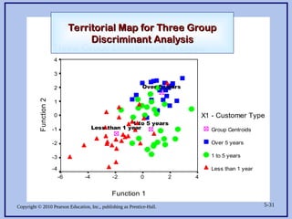
Figure 5.9 Territoral Map For
Three Group Discriminant Analysis
Function 1
4
2
0
-2
-4
-6
Function
2
4
3
2
1
0
-1
-2
-3
-4
X1 - Customer Type
Group Centroids
Over 5 years
1 to 5 years
Less than 1 year
Over 5 years
1 to 5 years
Less than 1 year
Territorial Map for Three Group
Territorial Map for Three Group
Discriminant Analysis
Discriminant Analysis
- 32.
Copyright © 2010Pearson Education, Inc., publishing as Prentice-Hall. 5-32
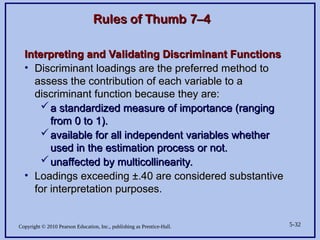
Rules of Thumb 7–4
Rules of Thumb 7–4
Interpreting and Validating Discriminant Functions
Interpreting and Validating Discriminant Functions
• Discriminant loadings are the preferred method to
Discriminant loadings are the preferred method to
assess the contribution of each variable to a
assess the contribution of each variable to a
discriminant function because they are:
discriminant function because they are:
a standardized measure of importance (ranging
a standardized measure of importance (ranging
from 0 to 1).
from 0 to 1).
available for all independent variables whether
available for all independent variables whether
used in the estimation process or not.
used in the estimation process or not.
unaffected by multicollinearity.
unaffected by multicollinearity.
• Loadings exceeding ±.40 are considered substantive
Loadings exceeding ±.40 are considered substantive
for interpretation purposes.
for interpretation purposes.
- 33.
Copyright © 2010Pearson Education, Inc., publishing as Prentice-Hall. 5-33
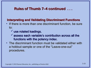
Rules of Thumb 7–4 continued . . .
Rules of Thumb 7–4 continued . . .
Interpreting and Validating Discriminant Functions
Interpreting and Validating Discriminant Functions
• If there is more than one discriminant function, be sure
If there is more than one discriminant function, be sure
to:
to:
use rotated loadings.
use rotated loadings.
assess each variable’s contribution across all the
assess each variable’s contribution across all the
functions with the potency index.
functions with the potency index.
• The discriminant function must be validated either with
The discriminant function must be validated either with
a holdout sample or one of the “Leave-one-out”
a holdout sample or one of the “Leave-one-out”
procedures.
procedures.
- 34.
Copyright © 2010Pearson Education, Inc., publishing as Prentice-Hall. 5-34
Stage 6: Validation of the Results
Stage 6: Validation of the Results
• Utilizing a Holdout Sample
Utilizing a Holdout Sample
• Cross-Validation
Cross-Validation
- 35.
Copyright © 2010Pearson Education, Inc., publishing as Prentice-Hall. 5-35
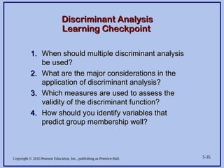
Discriminant Analysis
Discriminant Analysis
Learning Checkpoint
Learning Checkpoint
1.
1. When should multiple discriminant analysis
When should multiple discriminant analysis
be used?
be used?
2.
2. What are the major considerations in the
What are the major considerations in the
application of discriminant analysis?
application of discriminant analysis?
3.
3. Which measures are used to assess the
Which measures are used to assess the
validity of the discriminant function?
validity of the discriminant function?
4.
4. How should you identify variables that
How should you identify variables that
predict group membership well?
predict group membership well?
- 36.
Copyright © 2010Pearson Education, Inc., publishing as Prentice-Hall.
6-36
Variable Description
Variable Description Variable Type
Variable Type
Data Warehouse Classification Variables
Data Warehouse Classification Variables
X1
X1 Customer Type
Customer Type nonmetric
nonmetric
X2
X2 Industry Type
Industry Type nonmetric
nonmetric
X3
X3 Firm Size
Firm Size nonmetric
nonmetric
X4
X4 Region
Region nonmetric
nonmetric
X5
X5 Distribution System
Distribution System nonmetric
nonmetric
Performance Perceptions Variables
Performance Perceptions Variables
X6
X6 Product Quality
Product Quality metric
metric
X7
X7 E-Commerce Activities/Website
E-Commerce Activities/Website metric
metric
X8
X8 Technical Support
Technical Support metric
metric
X9
X9 Complaint Resolution
Complaint Resolution metric
metric
X10
X10 Advertising
Advertising metric
metric
X11
X11 Product Line
Product Line metric
metric
X12
X12 Salesforce Image
Salesforce Image metric
metric
X13
X13 Competitive Pricing
Competitive Pricing metric
metric
X14
X14 Warranty & Claims
Warranty & Claims metric
metric
X15
X15 New Products
New Products metric
metric
X16
X16 Ordering & Billing
Ordering & Billing metric
metric
X17
X17 Price Flexibility
Price Flexibility metric
metric
X18
X18 Delivery Speed
Delivery Speed metric
metric
Outcome/Relationship Measures
Outcome/Relationship Measures
X19
X19 Satisfaction
Satisfaction metric
metric
X20
X20 Likelihood of Recommendation
Likelihood of Recommendation metric
metric
X21
X21 Likelihood of Future Purchase
Likelihood of Future Purchase metric
metric
X22
X22 Current Purchase/Usage Level
Current Purchase/Usage Level metric
metric
X23
X23 Consider Strategic Alliance/Partnership in Future
Consider Strategic Alliance/Partnership in Future nonmetric
nonmetric
Description of HBAT Primary Database Variables
Description of HBAT Primary Database Variables
- 37.
Copyright © 2010Pearson Education, Inc., publishing as Prentice-Hall.
6-37
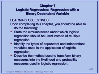
LEARNING OBJECTIVES
LEARNING OBJECTIVES
Upon completing this chapter, you should be able to
Upon completing this chapter, you should be able to
do the following:
do the following:
• State the circumstances under which logistic
State the circumstances under which logistic
regression should be used instead of multiple
regression should be used instead of multiple
regression.
regression.
• Identify the types of dependent and independent
Identify the types of dependent and independent
variables used in the application of logistic
variables used in the application of logistic
regression.
regression.
• Describe the method used to transform binary
Describe the method used to transform binary
measures into the likelihood and probability
measures into the likelihood and probability
measures used in logistic regression.
measures used in logistic regression.
Chapter 7
Chapter 7
Logistic Regression: Regression with a
Logistic Regression: Regression with a
Binary Dependent Variable
Binary Dependent Variable
- 38.
Copyright © 2010Pearson Education, Inc., publishing as Prentice-Hall.
6-38
LEARNING OBJECTIVES continued . . .
LEARNING OBJECTIVES continued . . .
Upon completing this chapter, you should be able to
Upon completing this chapter, you should be able to
do the following:
do the following:
• Interpret the results of a logistic regression
Interpret the results of a logistic regression
analysis and assessing predictive accuracy, with
analysis and assessing predictive accuracy, with
comparisons to both multiple regression and
comparisons to both multiple regression and
discriminant analysis.
discriminant analysis.
• Understand the strengths and weaknesses of
Understand the strengths and weaknesses of
logistic regression compared to discriminant
logistic regression compared to discriminant
analysis and multiple regression.
analysis and multiple regression.
Chapter 7
Chapter 7
Logistic Regression: Regression with a
Logistic Regression: Regression with a
Binary Dependent Variable
Binary Dependent Variable
- 39.
Copyright © 2010Pearson Education, Inc., publishing as Prentice-Hall.
6-39
Logistic Regression . . . is a specialized
Logistic Regression . . . is a specialized
form of regression that is designed to predict
form of regression that is designed to predict
and explain a binary (two-group) categorical
and explain a binary (two-group) categorical
variable rather than a metric dependent
variable rather than a metric dependent
measure. Its variate is similar to regular
measure. Its variate is similar to regular
regression and made up of metric
regression and made up of metric
independent variables. It is less affected than
independent variables. It is less affected than
discriminant analysis when the basic
discriminant analysis when the basic
assumptions, particularly normality of the
assumptions, particularly normality of the
independent variables, are not met.
independent variables, are not met.
Logistic Regression Defined
Logistic Regression Defined
- 40.
Copyright © 2010Pearson Education, Inc., publishing as Prentice-Hall.
6-40
Logistic Regression May Be Preferred . . .
Logistic Regression May Be Preferred . . .
When the dependent variable has only two groups, logistic
When the dependent variable has only two groups, logistic
regression may be preferred for two reasons:
regression may be preferred for two reasons:
• Discriminant analysis assumes multivariate normality and equal
Discriminant analysis assumes multivariate normality and equal
variance-covariance matrices across groups, and these
variance-covariance matrices across groups, and these
assumptions are often not met. Logistic regression does not
assumptions are often not met. Logistic regression does not
face these strict assumptions and is much more robust when
face these strict assumptions and is much more robust when
these assumptions are not met, making its application
these assumptions are not met, making its application
appropriate in many situations.
appropriate in many situations.
• Even if the assumptions are met, some researchers prefer
Even if the assumptions are met, some researchers prefer
logistic regression because it is similar to multiple regression. It
logistic regression because it is similar to multiple regression. It
has straightforward statistical tests, similar approaches to
has straightforward statistical tests, similar approaches to
incorporating metric and nonmetric variables and nonlinear
incorporating metric and nonmetric variables and nonlinear
effects, and a wide range of diagnostics.
effects, and a wide range of diagnostics.
- 41.
Copyright © 2010Pearson Education, Inc., publishing as Prentice-Hall.
6-41
Logistic Regression Decision Process
Logistic Regression Decision Process
Stage 1: Objectives of Logistic Regression
Stage 1: Objectives of Logistic Regression
Stage 2: Research Design for Logistic Regression
Stage 2: Research Design for Logistic Regression
Stage 3: Assumptions of Logistic Regression
Stage 3: Assumptions of Logistic Regression
Stage 4: Estimation of the Logistic Regression Model
Stage 4: Estimation of the Logistic Regression Model
and Assessing Overall Fit
and Assessing Overall Fit
Stage 5: Interpretation of the Results
Stage 5: Interpretation of the Results
Stage 6: Validation of the Results
Stage 6: Validation of the Results
- 42.
Copyright © 2010Pearson Education, Inc., publishing as Prentice-Hall.
6-42
Logistic regression is best suited to address
Logistic regression is best suited to address
two research objectives . . .
two research objectives . . .
• Identifying the independent variables that
Identifying the independent variables that
impact group membership in the dependent
impact group membership in the dependent
variable.
variable.
• Establishing a classification system based on
Establishing a classification system based on
the logistic model for determining group
the logistic model for determining group
membership.
membership.
Stage 1: Objectives of Logistic Regression
Stage 1: Objectives of Logistic Regression
- 43.
Copyright © 2010Pearson Education, Inc., publishing as Prentice-Hall.
6-43
Stage 2: Research Design for
Stage 2: Research Design for
Logistic Regression
Logistic Regression
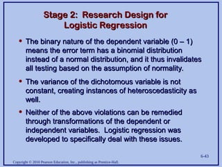
• The binary nature of the dependent variable (0 – 1)
The binary nature of the dependent variable (0 – 1)
means the error term has a binomial distribution
means the error term has a binomial distribution
instead of a normal distribution, and it thus invalidates
instead of a normal distribution, and it thus invalidates
all testing based on the assumption of normality.
all testing based on the assumption of normality.
• The variance of the dichotomous variable is not
The variance of the dichotomous variable is not
constant, creating instances of heteroscedasticity as
constant, creating instances of heteroscedasticity as
well.
well.
• Neither of the above violations can be remedied
Neither of the above violations can be remedied
through transformations of the dependent or
through transformations of the dependent or
independent variables. Logistic regression was
independent variables. Logistic regression was
developed to specifically deal with these issues.
developed to specifically deal with these issues.
- 44.
Copyright © 2010Pearson Education, Inc., publishing as Prentice-Hall.
6-44
Stage 3: Assumptions of
Stage 3: Assumptions of
Logistic Regression
Logistic Regression
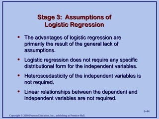
• The advantages of logistic regression are
The advantages of logistic regression are
primarily the result of the general lack of
primarily the result of the general lack of
assumptions.
assumptions.
• Logistic regression does not require any specific
Logistic regression does not require any specific
distributional form for the independent variables.
distributional form for the independent variables.
• Heteroscedasticity of the independent variables is
Heteroscedasticity of the independent variables is
not required.
not required.
• Linear relationships between the dependent and
Linear relationships between the dependent and
independent variables are not required.
independent variables are not required.
- 45.
Copyright © 2010Pearson Education, Inc., publishing as Prentice-Hall.
6-45
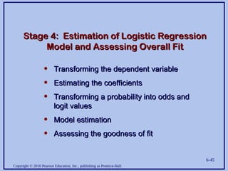
Stage 4: Estimation of Logistic Regression
Stage 4: Estimation of Logistic Regression
Model and Assessing Overall Fit
Model and Assessing Overall Fit
• Transforming the dependent variable
Transforming the dependent variable
• Estimating the coefficients
Estimating the coefficients
• Transforming a probability into odds and
Transforming a probability into odds and
logit values
logit values
• Model estimation
Model estimation
• Assessing the goodness of fit
Assessing the goodness of fit
- 46.
Copyright © 2010Pearson Education, Inc., publishing as Prentice-Hall.
6-46
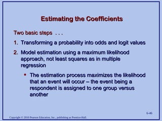
Estimating the Coefficients
Estimating the Coefficients
Two basic steps . . .
Two basic steps . . .
1.
1. Transforming a probability into odds and logit values
Transforming a probability into odds and logit values
2.
2. Model estimation using a maximum likelihood
Model estimation using a maximum likelihood
approach, not least squares as in multiple
approach, not least squares as in multiple
regression
regression
• The estimation process maximizes the likelihood
The estimation process maximizes the likelihood
that an event will occur – the event being a
that an event will occur – the event being a
respondent is assigned to one group versus
respondent is assigned to one group versus
another
another
- 47.
Copyright © 2010Pearson Education, Inc., publishing as Prentice-Hall.
6-47
Transforming a Probability into
Transforming a Probability into
Odds and Logit Values
Odds and Logit Values
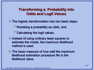
o The logistic transformation has two basic steps:
The logistic transformation has two basic steps:
Restating a probability as odds, and
Restating a probability as odds, and
Calculating the logit values.
Calculating the logit values.
o Instead of using ordinary least squares to
Instead of using ordinary least squares to
estimate the model, the maximum likelihood
estimate the model, the maximum likelihood
method is used.
method is used.
o The basic measure of how well the maximum
The basic measure of how well the maximum
likelihood estimation procedure fits is the
likelihood estimation procedure fits is the
likelihood value.
likelihood value.
- 48.
Copyright © 2010Pearson Education, Inc., publishing as Prentice-Hall.
6-48
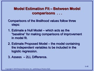
Model Estimation Fit – Between Model
Model Estimation Fit – Between Model
comparisons . . .
comparisons . . .
Comparisons of the likelihood values follow three
Comparisons of the likelihood values follow three
steps:
steps:
1.
1. Estimate a Null Model – which acts as the
Estimate a Null Model – which acts as the
“baseline” for making comparisons of improvement
“baseline” for making comparisons of improvement
in model fit.
in model fit.
2.
2. Estimate Proposed Model – the model containing
Estimate Proposed Model – the model containing
the independent variables to be included in the
the independent variables to be included in the
logistic regression.
logistic regression.
3.
3. Assess – 2LL Difference.
Assess – 2LL Difference.
- 49.
Copyright © 2010Pearson Education, Inc., publishing as Prentice-Hall.
6-49
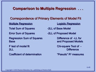
Comparison to Multiple Regression . . .
Comparison to Multiple Regression . . .
Correspondence of Primary Elements of Model Fit
Correspondence of Primary Elements of Model Fit
Multiple Regression
Multiple Regression Logistic Regression
Logistic Regression
Total Sum of Squares
Total Sum of Squares -2LL of Base Model
-2LL of Base Model
Error Sum of Squares
Error Sum of Squares -2LL of Proposed Model
-2LL of Proposed Model
Regression Sum of Squares
Regression Sum of Squares Difference of -LL for
Difference of -LL for
Base
Base and Proposed Models
and Proposed Models
F test of model fit
F test of model fit Chi-square Test of -
Chi-square Test of -
2LL
2LL Difference
Difference
Coefficient of determination
Coefficient of determination “Pseudo” R
“Pseudo” R2
2
measures
measures
- 50.
Copyright © 2010Pearson Education, Inc., publishing as Prentice-Hall.
6-50
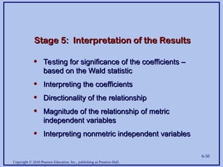
Stage 5: Interpretation of the Results
Stage 5: Interpretation of the Results
• Testing for significance of the coefficients –
Testing for significance of the coefficients –
based on the Wald statistic
based on the Wald statistic
• Interpreting the coefficients
Interpreting the coefficients
• Directionality of the relationship
Directionality of the relationship
• Magnitude of the relationship of metric
Magnitude of the relationship of metric
independent variables
independent variables
• Interpreting nonmetric independent variables
Interpreting nonmetric independent variables
- 51.
Copyright © 2010Pearson Education, Inc., publishing as Prentice-Hall.
6-51
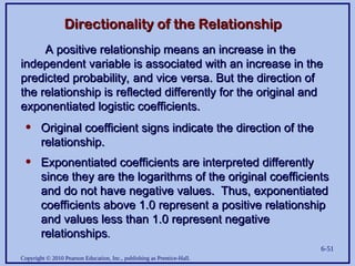
Directionality of the Relationship
Directionality of the Relationship
A positive relationship means an increase in the
A positive relationship means an increase in the
independent variable is associated with an increase in the
independent variable is associated with an increase in the
predicted probability, and vice versa. But the direction of
predicted probability, and vice versa. But the direction of
the relationship is reflected differently for the original and
the relationship is reflected differently for the original and
exponentiated logistic coefficients.
exponentiated logistic coefficients.
• Original coefficient signs indicate the direction of the
Original coefficient signs indicate the direction of the
relationship.
relationship.
• Exponentiated coefficients are interpreted differently
Exponentiated coefficients are interpreted differently
since they are the logarithms of the original coefficients
since they are the logarithms of the original coefficients
and do not have negative values. Thus, exponentiated
and do not have negative values. Thus, exponentiated
coefficients above 1.0 represent a positive relationship
coefficients above 1.0 represent a positive relationship
and values less than 1.0 represent negative
and values less than 1.0 represent negative
relationships
relationships.
.
- 52.
Copyright © 2010Pearson Education, Inc., publishing as Prentice-Hall.
6-52
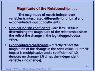
Magnitude of the Relationship . . .
Magnitude of the Relationship . . .
The magnitude of metric independent
The magnitude of metric independent
variables is interpreted differently for original and
variables is interpreted differently for original and
exponentiated logistic coefficients:
exponentiated logistic coefficients:
• Original logistic coefficients
Original logistic coefficients – are less useful in
– are less useful in
determining the magnitude of the relationship since
determining the magnitude of the relationship since
the reflect the change in the logit (logged odds)
the reflect the change in the logit (logged odds)
value.
value.
• Exponentiated coefficients
Exponentiated coefficients – directly reflect the
– directly reflect the
magnitude of the change in the odds value. But their
magnitude of the change in the odds value. But their
impact is multiplicative and a coefficient of 1.0
impact is multiplicative and a coefficient of 1.0
denotes no change (1.0 times the independent
denotes no change (1.0 times the independent
variable = no change).
variable = no change).
- 53.
Copyright © 2010Pearson Education, Inc., publishing as Prentice-Hall.
6-53
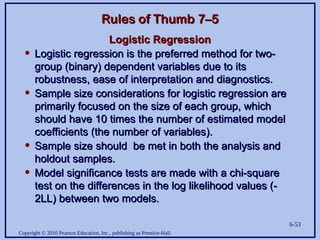
Rules of Thumb 7–5
Rules of Thumb 7–5
Logistic Regression
Logistic Regression
• Logistic regression is the preferred method for two-
Logistic regression is the preferred method for two-
group (binary) dependent variables due to its
group (binary) dependent variables due to its
robustness, ease of interpretation and diagnostics.
robustness, ease of interpretation and diagnostics.
• Sample size considerations for logistic regression are
Sample size considerations for logistic regression are
primarily focused on the size of each group, which
primarily focused on the size of each group, which
should have 10 times the number of estimated model
should have 10 times the number of estimated model
coefficients (the number of variables).
coefficients (the number of variables).
• Sample size should be met in both the analysis and
Sample size should be met in both the analysis and
holdout samples.
holdout samples.
• Model significance tests are made with a chi-square
Model significance tests are made with a chi-square
test on the differences in the log likelihood values (-
test on the differences in the log likelihood values (-
2LL) between two models.
2LL) between two models.
- 54.
Copyright © 2010Pearson Education, Inc., publishing as Prentice-Hall.
6-54
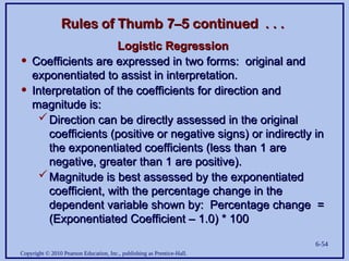
Rules of Thumb 7–5 continued . . .
Rules of Thumb 7–5 continued . . .
Logistic Regression
Logistic Regression
• Coefficients are expressed in two forms: original and
Coefficients are expressed in two forms: original and
exponentiated to assist in interpretation.
exponentiated to assist in interpretation.
• Interpretation of the coefficients for direction and
Interpretation of the coefficients for direction and
magnitude is:
magnitude is:
Direction can be directly assessed in the original
Direction can be directly assessed in the original
coefficients (positive or negative signs) or indirectly in
coefficients (positive or negative signs) or indirectly in
the exponentiated coefficients (less than 1 are
the exponentiated coefficients (less than 1 are
negative, greater than 1 are positive).
negative, greater than 1 are positive).
Magnitude is best assessed by the exponentiated
Magnitude is best assessed by the exponentiated
coefficient, with the percentage change in the
coefficient, with the percentage change in the
dependent variable shown by: Percentage change =
dependent variable shown by: Percentage change =
(Exponentiated Coefficient – 1.0) * 100
(Exponentiated Coefficient – 1.0) * 100
- 55.
Copyright © 2010Pearson Education, Inc., publishing as Prentice-Hall.
6-55
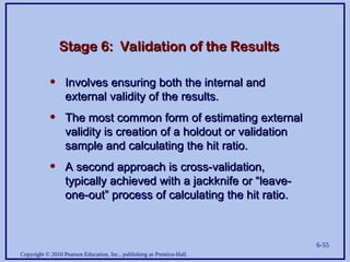
Stage 6: Validation of the Results
Stage 6: Validation of the Results
• Involves ensuring both the internal and
Involves ensuring both the internal and
external validity of the results.
external validity of the results.
• The most common form of estimating external
The most common form of estimating external
validity is creation of a holdout or validation
validity is creation of a holdout or validation
sample and calculating the hit ratio.
sample and calculating the hit ratio.
• A second approach is cross-validation,
A second approach is cross-validation,
typically achieved with a jackknife or “leave-
typically achieved with a jackknife or “leave-
one-out” process of calculating the hit ratio.
one-out” process of calculating the hit ratio.
- 56.
Copyright © 2010Pearson Education, Inc., publishing as Prentice-Hall.
6-56
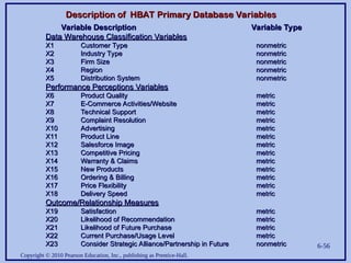
Variable Description
Variable Description Variable Type
Variable Type
Data Warehouse Classification Variables
Data Warehouse Classification Variables
X1
X1 Customer Type
Customer Type nonmetric
nonmetric
X2
X2 Industry Type
Industry Type nonmetric
nonmetric
X3
X3 Firm Size
Firm Size nonmetric
nonmetric
X4
X4 Region
Region nonmetric
nonmetric
X5
X5 Distribution System
Distribution System nonmetric
nonmetric
Performance Perceptions Variables
Performance Perceptions Variables
X6
X6 Product Quality
Product Quality metric
metric
X7
X7 E-Commerce Activities/Website
E-Commerce Activities/Website metric
metric
X8
X8 Technical Support
Technical Support metric
metric
X9
X9 Complaint Resolution
Complaint Resolution metric
metric
X10
X10 Advertising
Advertising metric
metric
X11
X11 Product Line
Product Line metric
metric
X12
X12 Salesforce Image
Salesforce Image metric
metric
X13
X13 Competitive Pricing
Competitive Pricing metric
metric
X14
X14 Warranty & Claims
Warranty & Claims metric
metric
X15
X15 New Products
New Products metric
metric
X16
X16 Ordering & Billing
Ordering & Billing metric
metric
X17
X17 Price Flexibility
Price Flexibility metric
metric
X18
X18 Delivery Speed
Delivery Speed metric
metric
Outcome/Relationship Measures
Outcome/Relationship Measures
X19
X19 Satisfaction
Satisfaction metric
metric
X20
X20 Likelihood of Recommendation
Likelihood of Recommendation metric
metric
X21
X21 Likelihood of Future Purchase
Likelihood of Future Purchase metric
metric
X22
X22 Current Purchase/Usage Level
Current Purchase/Usage Level metric
metric
X23
X23 Consider Strategic Alliance/Partnership in Future
Consider Strategic Alliance/Partnership in Future nonmetric
nonmetric
Description of HBAT Primary Database Variables
Description of HBAT Primary Database Variables

![Copyright © 2010 Pearson Education, Inc., publishing as Prentice-Hall. 5-24
Classification Matrix
Classification Matrix
HBAT’s New Consumer Product
HBAT’s New Consumer Product
Actual
Actual
Group
Group
Would
Would
Purchase
Purchase
Would
Would
Not
Not
Purchase
Purchase
Actual
Actual
Total
Total
Percent
Percent
Correct
Correct
Classification
Classification
Predicted Group
Predicted Group
Percent Correctly Classified (hit ratio) =
Percent Correctly Classified (hit ratio) =
100 x [(22 + 20)/50] = 84%
100 x [(22 + 20)/50] = 84%
(1)
(1) 22
22 3
3 25
25
88%
88%
(2)
(2) 5
5 20
20 25
25
80%
80%
Predicted
Predicted
Total
Total
27
27 23
23 50
50](https://image.slidesharecdn.com/chapter07discriminantlogistic-250516222532-22204780/85/Chapter-07-_discriminant-logistihjc-ppt-24-320.jpg)