or intro

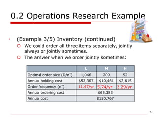
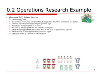
1. 1
0.1 Operations Research Concept
 Operations Research (Management Science) is a
scientific approach to decision making that seeks to
best design and operate a system
 We want to maximize ….
 Problem Example
 How to make highways.
 How to design a computer network.
 How to schedule doctors and nurses in a hospital
 How to mix raw materials (metals, chemicals, oil) to meet
the demand and to maximize the profit.
 Where to invest and when to invest.
 How to place advertisements on Super Bowl and a soap
opera under budget constraints.

2. 2
0.2 Operations Research Example
 (Example 1/5) Production
 Each year, Rylon has 6000 hrs of lab time
 Each year, Rylon can buy 4000 lb of raw material.
 How much of each product should we make to maximize the
profit?
1 lb raw
material
3 oz
Brute
4 oz
Chanelle
and
1hr/lb
Reg. Brute
Lux. Brute
Reg. Chan
Lux. Chan
$7/oz
$6/oz
3hr/oz
$4/oz
2hr/oz
$4/oz
$18/oz
$14/oz
or
or
$3/lb

3. 3
0.2 Operations Research Example
 (Example 2/5) Investment
 Finco can invest in five opportunities.
 Cash flows are given below.
 Currently FI has $100,000 (at the end of time zero).
 Any investment cannot use more than $75,000
(portfolio diversification).
 Any income can be re-invested right away.
 We want to maximize the money
value at the END of period 3.
 Which options to take?
 Can you guess what to do if we
have 100 options over 60
months?
Opt. 0 1 2 3
A -1 0.5 1 0
B 0 -1 0.5 1
C -1 1.2 0 0
D -1 0 0 1.9
E 0 0 -1 1.5

4. 4
0.2 Operations Research Example
 (Example 3/5) Inventory
 We have three products: L, M, H.
 Demand: DL
=12,000/yr, DM
=1,200/yr, DH
=120/yr
 We want to minimize the inventory cost (set up+holding)
 Common order cost: S=$4,000
 Product specific order cost: sL
=sM
=sH
=$1,000
 Product unit cost: pL
=pM
=pH
(or cL
=cM
=cH
)=$500
 Holding cost rate: h= $100/item/yr
 When to order? How much to order each time?
S
(truck shipping)
si
order picking

5. 5
0.2 Operations Research Example
 (Example 3/5) Inventory (continued)
 We could order all three items separately, jointly
always or jointly sometimes.
 The answer when we order jointly sometimes:
L M H
Optimal order size (D/n*) 1,046 209 52
Annual holding cost $52,307 $10,461 $2,615
Order frequency (n*) 11.47/yr 5.74/yr 2.29/yr
Annual ordering cost $65,383
Annual cost $130,767

6. 6
0.2 Operations Research Example
 (Example 4/5) Gambling
 Each time, we win or lose, based on luck.
 The chance of winning each time is 45%. We lose with 55% of chance.
 When we have either $0 or $70, we leave.
 What is the chance we leave with a fortune?
 This is an example of a random walk.
 Is a life or business a series of gambles?
$0 $10 $20 $30 $40 $50 $60 $70

7. 7
0.2 Operations Research Example
 (Example 5/5) Patient Service
 Colonoscopy area.
 Six operation rooms, two admission RNs, five operation RNs, three technicians, two doctors.
 Different procedure time depending on operation type.
 Patients are sometimes late or no-show.
 We want to max the profit and min patients’ waiting time.
 Effect of inter-appointment time? What if we do not have an appointment system?
 Effect of more or fewer people of each resource type?
 Dedicated doctor to a patient or not dedicated?

8. 8
0.3 Operations Research Application
 Possible application areas of OR
 Finance
 Marketing
 E-business
 Telecommunications
 Games (Industrial games, Duopoly, Economy)
 Operations Management
 Production Planning
 Transportation Planning
 System Design
 Health care
 National security
 (and many more)

9. 9
0.4 Operations Research History
 During WW II, British military asked scientists/
engineers to analyze several military problems.
 Deployment of radar
 Management of convoy, bombing, antisubmarine, and
mining operations.
 The result was called Military Operations Research,
later Operations Research
 Now the scope is getting larger as
 Efficiency gets more important in military & industry
 Computer becomes more powerful
 More data are available (e-business, ERP/SCM, etc)

10. 10
0.6 Areas of Operations Research
1. Analytical approach: Math Programming
 LP (Linear Programming)
 NLP (Non Linear Programming) (Max x2+xy2. st. x2 ≤ 1)
 IP (Integer Programming) (x is an integer variable)
 Quadratic programming (x2 or xy; no x3 or log x)
x1:#desks, x2:#tables to make
Objective function Maximize z(profit)=3 x1 + 4 x2
Constraint 1 (desk raw material) 5 x1 ≤ 100
Constraint 2 (table raw material) 3 x2 ≤ 150
Constraint 3 (labor constraint) 3 x1 + 4 x2 ≤ 900
Non-negativity constraint x1, x2 ≥ 0

11. 11
0.6 Areas of Operations Research
2. Analytical approach: Others
 Queuing Theory: waiting line
 Where do we see queues?
 Do you not like waiting?
 Inventory Theory
 How many groceries do we buy a year?
 At grocery shopping, how much do we buy each time?
One apple each time every day (or every five minutes)
or one year’s supply?
 Stochastic Process (uncertainties: stock market, gambling)
 Scheduling: assignment of resources over time
 Examples of resources in scheduling?
 DP (Dynamic Prog), Game theory, Reliability (HW/SW)
3. Simulation approach: Computer Q simulation

12. 12
 The scientific approach to decision making
requires the use of mathematical models.
 A mathematical model is a mathematical
representation of an actual situation for better
clarification or better decisions of the situation.
 Reason for modeling: too complicated or expensive
 Physical vs. Computer Model (Wind tunnel, FEM)
 Analytical model vs. Simulation model
heat
or force
0.7 Modeling Concept

13. 13
0.7 Modeling Concept
 The more accurate, the better? No!
 Balance between desired accuracy and modeling cost
 E.g., Do we model machine failure or
volume discount?
 Planning by each product or product group?
Real
System
Simplified
System
LP
formulation
Solution
Interpret
ation
Modeling
(assumptions,
validation)
LP language
(LP format)
By hand or
Computer
LP theory
Remodeling

14. 14
0.7 Modeling Concept
 Meaning of Optimal Solution
 OR seeks the optimal solution.
 Best Solution (Theoretically proven) vs. Good solution
 Optimal to the formulation or to the model (not
to the real problem)
 Model validation is important.
 Validation: checking if the model correctly
represents the actual case to the degree we want.

15. 15
0.8 Performance measure
 When we compare the performance of different
solutions, what numerical values do we compare?
(or equivalently,)
 What do we want to achieve?
 This is called performance measure.
 Example
 Maximize profit. Minimize cost.
 Minimize inventory. Minimize flow time.
 Minimize lateness of orders.

16. 16
0.9 Solution procedure
 Algorithm
 Systematic solution procedure
 Iterative procedure
 Computer in mind
 Good algorithm: fast and less memory requirement
 Complexity of an algorithm: # iterations needed
1 3 4 2 1 2 3 4