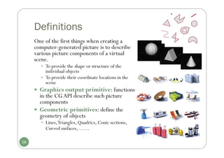
Chapter 3 discusses computer graphics software, focusing on various graphics software packages, including OpenGL, and important graphic functionalities and algorithms. It covers the graphics rendering process, coordinate systems, and provides a detailed introduction to OpenGL with its syntax and utility functions. The chapter concludes by highlighting the architecture of the graphics rendering pipeline and foundational concepts for output primitives and rasterization.

1. Chapter 3
Computer Graphics Software
Computer Graphics

2. Outline
 Graphics Software Packages
 Introduction to OpenGL
 Example Program
2

3. Graphics Software
3
 Software packages
 General Programming Graphics Packages
 GL (Graphics Library, 1980s) [SGI], OpenGL(1992), GKS (Graphical
Kernel System, 1984), PHIGS (Programmer’s Hierarchical Interactive
Graphics System), PHIGS+,VRML(superseded by X3D), Direct3D,
Java2D/Java3D
 Special - Purpose Application Packages
 CAD /CAM, Business, Medicine,Arts ( forAnimation: 3ds Max, Maya
[Autodesk, originallyAlias (formerlyAlias|Wavefront)] )
 Computer-graphics application programming interface (CG
API)
 A set of graphics functions to let programmers control hardware
 A software interface between a programming language and the hardware.
 E.g.: GL, OpenGL, Direct3D

4. Functions of Graphics Packages
 Functions provided by general graphics packages are to
create and manipulate pictures
 Graphics Output Primitives: lines, curves, spheres…
 PrimitiveAttributes: color, line styles…
 GeometricTransformations
 ViewingTransformations
 Input Functions: data flow from mouse, joystick, …
 Control Operations
4

5. Algorithms
 A number of basic algorithms are needed:
 Transformation: convert models/primitives from one coordinate system
to another
 Clipping/Hidden surface removal: remove primitives and part of
primitives that are not visible on the display
 Rasterization: convert a projected screen space primitive to a set of pixels.
 Advanced:
 Shading and illumination: simulate the highly realistic lighting effect of
a scene.
 Animation: simulate movement by rendering a sequence of frames.
 Parallel processing & real time rendering for graphics computation,
in particular to large and/or natural environments.
 Physically based graphics modeling and rendering.
5

6. Graphics Rendering Process
 Rendering purpose: the conversion of a 3D scene into a
2D image
render
2D Image
6
Graphics Rendering Pipeline
Fixed graphics Pipeline in
hardware
Programmable pipeline in
hardware

7.  Modeling (local/master) coordinates (MC)
A separate coordinates reference frame for object.
 Local coordinate system (2D or 3D)
 Define the coordinates for each object individually
 Scale and unit are varied from object to object
 World coordinates (WC)
A scene reference frame where the objects are placed at appropriate locations.
 Global coordinate system (2D or 3D)
 Place all defined objects together in a scene within this reference system
 MC WC (modeling transformation)
Coordinate (坐標) Representations in
Graphics Rendering Pipeline
7

8.  Viewing and projection coordinates
 World coordinates positions are transformed though the viewing pipeline to viewing and
projection coordinates. (Viewing transformation)
 Normalized (device) coordinates (NC)
 Make coordinate independent to any specific output device (device-independent)
 The scene is stored in normalized coordinates, range from -1 to 1, or 0 to 1.
 Stage betweenWC and DC
 Device (screen) coordinate (DC)
 Display coordinate system on the output device (e.g, screen)
 2D only
 Platform dependent
8
Coordinate Representations in Graphics
Rendering Pipeline

9. Graphics Rendering Pipeline
9
Model
Model
Model
M1
M2
M3
3D World
Scene
3D View
Scene
V
P Clip Normalize
2D/3D Device
Scene
2D Image
Projection
Rasterization
Modeling
Transformations
Viewing
Transformations
MCS
WCS
VCS
NDCS
DCS
SCS
(From CENG477 notes,09)

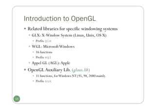
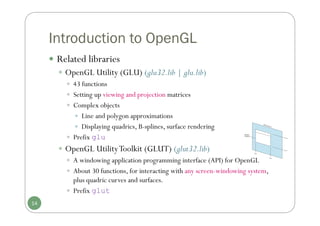
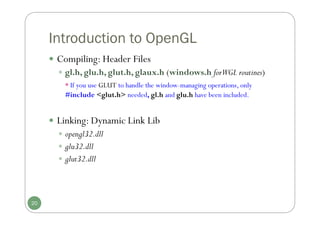
10. Introduction to OpenGL
 OpenGL (Open Graphics Library)
[developed by Silicon Graphics Inc.(SGI) in 1992,and maintained by OpenGL
Architectural Review Board (OpenGL ARB),the group of companies that would maintain
and expand the OpenGL specification until 2006;by Khronos Group until now ]
10
 Khronos Group (http://www.khronos.org/)
[a nonprofit industry consortium creating open standards for the
authoring and acceleration of parallel computing, graphics, dynamic
media, computer vision and sensor processing on a wide variety of
platforms and devices. ]

11. Introduction to OpenGL
 OpenGL (Open Graphics Library)
 A common graphics library which provides functions for
drawings and interactive input.
 A cross-language, cross-platformAPI
 No command for performing windowing tasks
 No command for handling input
 Accessible via C/C++, Java…
http://www.opengl.org
11

12. Introduction to OpenGL
 OpenGL basic (core) library (opengl32.lib | opengl.lib)
 Over 250 functions, specifying objects and operations needed to
produce interactive 3D graphics
 OpenGL geometric primitives include points, lines and polygons;
specific support for triangle and quadrilateral polygons; quadric
(defined by quadratic equation) and NURBES (spline) surface.
 Texture mapping support.
 ……
 From OpenGL 2.0: Programmable shader support
12

13. Introduction to OpenGL
 Related libraries for specific windowing systems
 GLX: X-Window System (Linux, Unix, OS X)
 Prefix glx
 WGL: MicrosoftWindows
 16 functions
 Prefix wgl
 Appel GL (AGL):Apple
 OpenGLAuxiliary Lib. (glaux.lib)
 31 functions, forWindows NT|95, 98, 2000 mainly.
 Prefix aux
13

14. Introduction to OpenGL
 Related libraries
 OpenGL Utility (GLU) (glu32.lib | glu.lib)
 43 functions
 Setting up viewing and projection matrices
 Complex objects
 Line and polygon approximations
 Displaying quadrics, B-splines, surface rendering
 Prefix glu
 OpenGL UtilityToolkit (GLUT) (glut32.lib)
 A windowing application programming interface (API) for OpenGL
 About 30 functions, for interacting with any screen-windowing system,
plus quadric curves and surfaces.
 Prefix glut
14

15. OpenGL Utility Toolkit (GLUT)
-Written by Mark Kilgard formerly in SGI, now in NVIDIA
 A window-system independent toolkit
 NOT a part of OpenGL
 BUT a windowingAPI for OpenGL, so no need to know
 The details of different platform: GLX,WGL, andAGL
 The details of opening a window and an OpenGL context across operating
systems.
 The details of various input devices, such as keyboard and mouse.
 Widely used in demonstration programs and literature.
15

16. GLUT – Hello World
 Open a window
16
display function is defined as
void (*func) (void)
{ };
A callback function which is registered by
glutDisplayFunc as a routine to invoke when
the window need to be redisplayed.

17. OpenGL Syntax
 Functions, symbols, and types
glBegin, glClear, glCopyPixels, glPolygonMode
GL_2D, GL_POLYGON, GL_BUFFER_BIT
GLbyte, GLshort, GLint, GLfloat, GLdouble
 Prefix gl
 Each component word in the function name has its first letter
capitalized
 Arguments are assigned symbolic constants specifying
parameter names, values of parameters, or a mode.
 Constants defined with GL_, and underscores separate words.
 OpenGL defines its own types which correspond to C types
GLbyte: signed char; GLshort:short; GLint: int; GLfloat: float…
17

18. OpenGL Syntax
 Functions are always named in the following manner
glColor3f(0.0f, 0.0f, 0.0f)
 gl + actual function name + number of arguments +
type of arguments
 Number of arguments: 2, 3, 4
 Type of arguments: s, i, f, d, ub, v… (v indicates it’s a
vector/array)
18

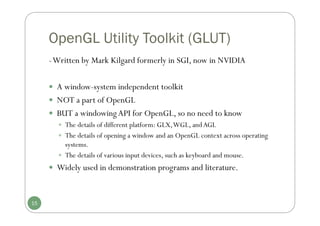
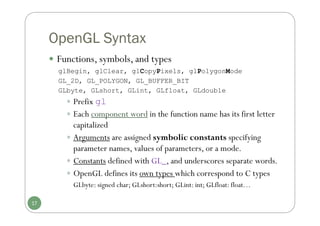
19. OpenGL Syntax
 Example
 glColor3f(0.0f, 0.4f, 0.8f);
This is: 0% Red, 40% Green, 80% Blue
 glColor4f(0.1, 0.3, 1.0, 0.5) ;
This is: 10% Red, 30% Green, 100% Blue, 50% Opacity
 GLfloat color[4] = {0.0, 0.2, 1.0, 0.5};
glColor4fv( color );
It is 0% Red, 20% Green, 100% Blue, 50% Opacity
19

20. Introduction to OpenGL
 Compiling: Header Files
 gl.h, glu.h, glut.h, glaux.h (windows.h forWGL routines)
* If you use GLUT to handle the window-managing operations, only
#include <glut.h> needed, gl.h and glu.h have been included.
 Linking: Dynamic Link Lib
 opengl32.dll
 glu32.dll
 glut32.dll
20

21. An Example of OpenGL
 Initialize OpenGL and GLUT
 Initialize a drawing window
 Draw a line segment
21

22. An Example of OpenGL
22

23. An Example of OpenGL
//give the initial location for the top-left corner of the display window
glutInitWindowPosition (50, 100);
//set the initial pixel width and height of the display window
glutCreateWindowSize (400, 300);
23
Figure 3-2 A 400 by 300 display
window at position (50, 100) relative to
the top-left corner of the video display.

24. End of Chapter 3
24

25. Summary
 Basic display devices
 Input devices
 Graphics software packages
 Graphics rendering pipeline and coordinate
representations
 OpenGL introduction
25

26. Chapter 4
Graphics Output Primitives
(Part I)
Computer Graphics

27. Outline
 Definition of graphics output primitives
 Coordinate Reference Frames
 OpenGL Point Functions
 OpenGL Line Functions
 Implementation Algorithm: Line-Drawing Algorithms
(Chapter 6)
 DDA
 Bresenham
27

28. Definitions
One of the first things when creating a
computer-generated picture is to describe
various picture components of a virtual
scene.
 To provide the shape or structure of the
individual objects
 To provide their coordinate locations in the
scene
 Graphics output primitive: functions
in the CGAPI describe such picture
components
 Geometric primitives: define the
geometry of objects
 Lines,Triangles, Quadrics, Conic sections,
Curved surfaces, ……
28

29. Coordinate Reference Frames
 World coordinate system
 Cartesian coordinates (笛卡尔坐标)
 A right hand coordinate system
 Label the axes as
 X (horizontal)
 Y (vertical)
 Z (in 3D)
 Origin is in the lower left
XAxis
Y Axis
(0,0) +X
+Y
29

30. Partition Space into Pixels
 Object information, such as the coordinates, colors, is passed to
the viewing routines.
 Map the 3D objects to positions on the 2D screen
 Scan-conversion methods
 Converts vector images (primitives such as lines, circles, etc.) into raster
images (integer pixel values)
 Geometric description  discrete pixel representation
30
Rasterization
(光柵化)

31. Screen Coordinate System
 Screen: 2D coordinate system (W*H)
 Two definitions for screen coordinate
system:
 For hardware processes, such as screen
refreshing, the origin is at the top-left
corner of the screen
 y - scan line number;
 x - column number.
 For software, the origin is at the low-left
corner (OpenGL convention)
 Correspond to the pixel positions in the
frame buffer
X Axis
Y Axis
(0,0) +X
+Y
31
Quick review:
What’s the pixel?

32. “pixel” is a screen spot.
From a geometry point of view, a pixel is a point.
Q: Where is the pixel P(2,1) on the screen?
2
2
1
1
0 3 4
3
5
32
How to represent each pixel position by the screen coordinates? Is it a square or a point?

33. Therefore, when we think about images, a pixel is a rectangle or the
inscribed circle.
Q: Where is P(2,1) on the screen? A: the center of a pixel located.
1
2
0
1
0 3 4
2
33

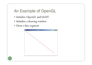
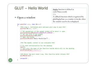
34. Basic OpenGL Point Structure
 In OpenGL, to specify a point:
 glVertex*(); (*) indicates the suffix codes needed
 glVertex2i(80, 100), glVertex2f(58.9, 90.3)
 glVertex3i(20, 20, -5), glVertex3f(-2.2, 20.9, 20)
 Must put within a‘glBegin/glEnd’ pair
glBegin(GL_POINTS);
glVertex2i(50, 100);
glVertex2i(75, 150);
glVertex2i(100, 200);
glEnd();
The form of a point position
in OpenGL spec.:
glBegin (GL_POINTS);
glVertex* ();
glEnd ();
34
[ gl + actual function name + number of arguments + type of arguments ]
Symbolic constant

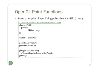
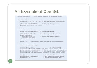
35. OpenGL Point Functions
 Some examples of specifying points in OpenGL
//Specify the coordinates of points in arrays; then call the OpenGL functions
int point1 [] = {50, 100};
int point2 [] = {75, 150};
int point3 [] = {100, 200};
glBegin (GL_POINTS);
glVertex2iv (point1);
glVertex2iv (point2);
glVertex2iv (point3);
glEnd ();
//Specify the points in 3D world reference frame
glBegin (GL_POINTS);
glVertex3f (-78.05, 909.72, 14.60);
glVertex3f (261.91, -5200.67, 188.33);
glEnd ();
35

36. OpenGL Point Functions
 Some examples of specifying points in OpenGL (cont.)
// In C++, define a C++ class or structure of a point
class wcPt2D {
public:
GLfloat x, y;
};
wcPt2D pointPos;
pointPos.x = 120.75;
pointPos.y = 45.30;
glBegin (GL_POINTS);
glVertex2f (pointPos.x, pointPos.y);
glEnd ();
36

37. OpenGL Line Functions
glBegin (GL_LINES);
glVertex2iv (p1);
glVertex2iv (p2);
glVertex2iv (p3);
glVertex2iv (p4);
glVertex2iv (p5);
glEnd ();
glBegin (GL_LINE_STRIP);
glVertex2iv (p1);
glVertex2iv (p2);
glVertex2iv (p3);
glVertex2iv (p4);
glVertex2iv (p5);
glEnd ();
p2
p1
p3
p4
p2
p1
p3
p4
p5
37
 In OpenGL, to specify one or more straight-line segments:

38. OpenGL Line Functions
glBegin (GL_LINE_LOOP);
glVertex2iv (p1);
glVertex2iv (p2);
glVertex2iv (p3);
glVertex2iv (p4);
glVertex2iv (p5);
glEnd ();
p2
p1
p3
p4
p5
38
 In OpenGL, to specify one or more straight-line segments
(cont.):

39. Implementation Algorithm:
Line drawing algorithms
Digital DifferentialAnalyzer (DDA)
Bresenham’s LineAlgorithm
39

40. Line-Drawing Algorithms
 The ideal line
 Continuous appearance
 Uniform thickness and brightness
 Line on a raster monitor
 Screen: discrete pixels
 Digitize the line into a set of discrete integer positions approximating
the actual line path.
40

41. Line-Drawing Algorithms
(17,8)
(2,2)
41
 Discretization - converting a continuous signal into discrete elements.
 Scan conversion line-drawing algorithm: convert the line information
into pixel data for display

42. Line-Drawing Algorithms
 How to calculate the pixel positions along a straight-line path
The line equation (slope-intercept equation): any point (x, y) on the
line must follow it.
y = m • x + b, where
 m is the slope (斜率) of the line.
 b is the intercept on y-axis.
 If we have two endpoints, (x0, y0) and (xend, yend), then m and b can
be calculated as:
m = y / x = (yend – y0) / (xend – x0)
b = y0 - m . x0
42

43. Line-Drawing Algorithms
 which is the nearest pixel to the line at each sampled position.
 Two line-drawing algorithms:
(1) DDA (Digital DifferentialAnalyzer).
(2) Bresenham’s LineAlgorithm.
43
 On raster system, the line is approximated by pixels. How
good it is, decided by:
 how to sample a line at discrete positions (step sizes of the
calculation in the horizontal (x) and vertical (y) directions)

44. (1) Line drawing – DDA algorithm
 (DDA) is a scan-conversion line algorithm based on calculating
either y or x.
 Each point is generated from the previous point
 Take a unit step with one coordinate and calculate the corresponding value
for another
 Slope of a line m = Δy/Δx
 y = m • x or x = y / m
 Different cases based on the sign of the slope, value of the slope,
and the direction of drawing.
 Slope sign: positive or negative.
 Slope value: <= 1 or >1.
 Direction: (left – right) or (right – left)
x
y
44
Four Quadrants
I
II
III IV

45. DDA algorithm
a low level procedure to store the current color
into the frame buffer at (x, y)
// if |m|<1, | ∆x | =1.
// if |m|>1, | ∆y | =1.
45
y = m • x
x = y / m

46. Line drawing – DDA algorithm
 DDA summary
1.Go to starting point
2.Increment x and y values
 Step size:
- one unit (in x or y direction)
- calculating corresponding value for another
3.Round to the closest raster position
 Merits
Relative fast: replace the multiplication by using the increments
of x or y directions to step from one pixel to another.
 Drawbacks
 Divisions needed to set increment values
 The use of floating-point arithmetic
 Rounding operations to an integer
46

47. (2) Bresenham’s Line Algorithm
 An efficient algorithm for line drawing
 Using only integer addition/subtraction
 We have a point (xk, yk), then at each
sampling step
 Two possible pixel positions: A (xk+1, yk)
and B (xk+1, yk+1)
 To decide which is closer to the line path
47
The vertical axes show scan-line
positions;
The horizontal axes identify pixel
columns.
A
B
dA
dB

48. Bresenham’s Line Algorithm for |m|<1.0
1. Input the two line endpoints and store the left one (x0, y0).
2. Plot (x0, y0) to be the first point (set the color for frame buffer position (x0,
y0)).
3. Calculate the constants ∆x, ∆y, 2∆y, and 2∆y – 2∆x, and obtain the starting
value for the decision parameter as p0 = 2∆ y – ∆x.
4. At each xk along the line, starting at k = 0, perform the following test.
If pk < 0,
plot (xk+1, yk) and pk+1 = pk + 2∆y
Otherwise,
plot (xk+1, yk+1) and pk+1 = pk + 2∆y – 2∆x.
5. Perform step 4 ∆x – 1 times.
48
yk+1
xk+1
y
dlower
dupper
yk A
B

49. Bresenham’s Line Algorithm Example
 Note:This Bresenham’s algorithm is used when slope |m|< 1.
Example 3-1: Using Bresenham’s Line-Drawing Algorithm, digitize the line with
endpoints (20,10) and (30,18).
-- y = 18 – 10 = 8
-- x = 30 – 20 = 10
-- m = y / x = 0.8
 plot the first point (x0, y0) = (20, 10)
 p0 = 2 y – x = 2 • 8 – 10 = 6 , so the next point is (21, 11)
The next point is (xk+1, yk+1)
49

50. K Pk (xk +1, yk +1) K Pk (xk +1, yk +1)
0 6 (21,11) 5 6 (26,15)
1 2 (22,12) 6 2 (27,16)
2 -2 (23,12) 7 -2 (28,16)
3 14 (24,13) 8 14 (29,17)
4 10 (25,14) 9 10 (30,18)
Pk > 0: Pk+1 = Pk + 2∆y – 2∆x Pk < 0: Pk+1 = Pk + 2∆y
50
 The successive pixel positions along the line path can be
determined from the decision parameter as
Bresenham’s Line Algorithm Example
y = 8; x = 10

51. Bresenham’s Line Algorithm Example
 Pixel positions along the line path between endpoints (20, 10)
and (30, 18), plotted with Bresenham’s algorithm.
51
(20, 10); (21,11); (22,12); (24,13); (25,14); …; (30,18).

52. Bresenham’s Line Algorithm for |m|<1.0
52
Pk > 0: Pk+1 = Pk + 2∆y – 2∆x
Pk < 0: Pk+1 = Pk + 2∆y

53. Setting Frame Buffer Values
 The final stage of line segment implementation is to set the frame-
buffer color values. Suppose:
 The frame buffer is stored in memory as an addressable array.
 The frame buffer array is stored row by row (row-major order).
 Pixel positions are labeled from (0,0) at the lower-left screen corner to
(xmax, ymax) at the top-right corner.
53
For a bilevel (one bit per pixel) system, the frame buffer bit address for the pixel
at (x, y): addr(x,y) = addr(0,0) + y•(xmax + 1) + x

54. Summary
 OpenGL output primitives functions
 Point and line
 Line drawing algorithm
 DDA
 Bresenham
54

55. END
55

56. DDA – case 1 (1st quadrant)
 Positive slope; left to right:
 If 0 <= m <= 1 then:
xk+1 = xk + 1
yk+1 = yk + m
(rounded to the nearest integer
corresponding to a screen pixel
position in x coordinate)
 If m > 1 then:
xk+1 = xk + 1/m
yk+1 = yk + 1
y = m • x
x = y / m
56
Four Quadrants
I

57. DDA – case 2 (3rd quadrant)
 Positive slope; right to left:
 If 0 < m <= 1 then:
xk+1 = xk – 1
yk+1 = yk – m
 If m > 1 then:
xk+1 = xk – 1/m
yk+1 = yk – 1
57
y = m • x
x = y / m
Four Quadrants
III

58. DDA – case 3 (4th quadrant)
 Negative slope; left to right:
 If |m | <= 1 then:
xk+1 = xk + 1
yk+1 = yk – |m|
 If |m | > 1 then:
xk+1 = xk + 1/|m|
yk+1 = yk – 1
58
y = m • x
x = y / m
Four Quadrants
IV

59. DDA – case 4 (2nd quadrant)
 Negative slope; right to left:
 If |m | <= 1 then:
xk+1 =
yk+1 =
 If |m | > 1 then:
xk+1 =
yk+1 =
59
y = m • x
x = y / m
Four Quadrants
xk – 1
yk + |m|
xk – 1/|m|
yk + 1
?
?
?
?
II

60. Bresenham’s Line Algorithm
Consider lines with positive slope less than 1.0:
 At sampling point xk+1, we label vertical pixel separations from
the mathematical line path as dlower and dupper.
 After calculating dlower and dupper we will choose yk or yk+1.
y = m (xk + 1) + b
dlower = y – yk = m (xk + 1) + b – yk
dupper = (yk+1) – y = yk+1 - m (xk + 1) – b
An efficient test:
dlower – dupper = 2m • xk + 2m – 2yk + 2b – 1
= 2m (xk + 1) – 2yk + 2b – 1
y = m x + b
60
A
B
C

61. Bresenham’s Line Algorithm
 To derive the decision parameter for the kth step: pk
 dlower – dupper = 2m (xk + 1) – 2yk + 2b – 1
 m = y / x
∆x (dlower – dupper ) = 2 ∆ y (xk + 1) – ∆ x (2yk – 2b +1)
= 2 ∆ y • x k – 2 ∆ x • yk + c
where c = 2 ∆ y + ∆ x (2b – 1) is a constant; and k
represents the kth step.
pk = ∆x (dlower – dupper ) = 2 ∆ y • x k – 2 ∆ x • yk + c
61

62. Bresenham’s Line Algorithm
pk = ∆x (dlower – dupper ) = 2 ∆ y • x k – 2 ∆ x • yk + c
 If pk < 0 (i.e. dlower < dupper)  we plot the pixel A (xk+1, yk)
Otherwise we plot the pixel B (xk+1, yk+1)
yk+1
xk+1
y
dlower
dupper
yk
62
A
B
C

63. Bresenham’s Line Algorithm
 Go on to the next step, we need to decide the pk+1: pk  pk+1
From pk = 2 ∆ y • x k – 2 ∆ x • yk + c, we can get
pk+1 = 2 ∆ y • x k+1 – 2 ∆ x • yk+1 + c,
where c = 2 ∆ y + ∆ x (2b – 1) is a constant
Therefore,
pk+1 – pk = 2 ∆ y (x k+1 – x k) – 2 ∆ x (yk+1 – yk )
 pk+1 = pk + 2 ∆y – 2 ∆x (yk+1 – yk)
 The first parameter p0 = 2 ∆ y – ∆ x
hint: from (x0, y0) and m= ∆y/ ∆ x, k = 0.
xk+1 = xk + 1
x0+1
y
dlower
dupper
y0+1
y0
0 or 1, depending on the sign of pk
63