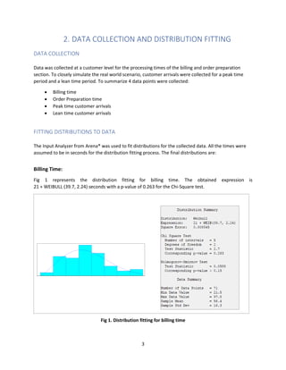
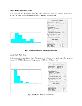
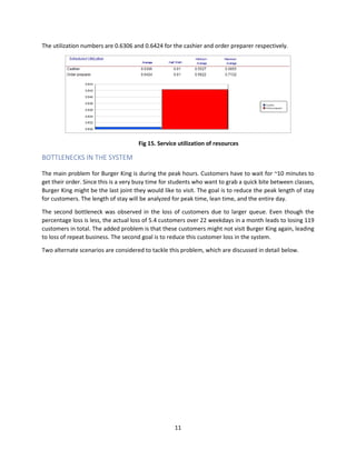
The Burger King Fast Food joint at Tangeman University Center is one of the main joints that UC students frequent to grab a quick bite. The store runs from 7 am to 7 pm on weekdays and for reduced hours on weekends. Majority of the business/ influx of students for the joint is observed on weekdays with the peak hours being 11 am to 3 pm. The project helped identify bottlenecks observed in the system during peak hours and suggested an alternate resource restructuring with the same man hours. A reduction of 53% in customer wait time was observed in the new solution. Arena® was chosen as the software to simulate the Burger King setup and identify areas of improvement.

1. Jain, Rohit (M12397009)
MS Business Analytics
12/03/2017
Burger King Simulation

2. 1
Table of Contents
1. PROJECT INTRODUCTION................................................................................................................2
INTRODUCTION AND OBJECTIVE ..............................................................................................................2
SYSTEM UNDERSTANDING........................................................................................................................2
ASSUMPTIONS ..........................................................................................................................................2
2. DATA COLLECTION AND DISTRIBUTION FITTING..............................................................................3
DATA COLLECTION ....................................................................................................................................3
FITTING DISTRIBUTIONS TO DATA ............................................................................................................3
USING THE NON-STATIONARY POISSION PROCESSS ................................................................................5
3. BASE MODEL ANALYSIS ..................................................................................................................6
GENERAL SETUP........................................................................................................................................6
BUILDING THE MODEL ..............................................................................................................................6
IDENTIFYING THE NUMBER OF REPLICATIONS.........................................................................................7
MODEL RESULTS: ......................................................................................................................................9
BOTTLENECKS IN THE SYSTEM................................................................................................................11
4. ANALYSIS OF ALTERNATE SCENARIOS ...........................................................................................12
DESCRIPTION OF THE ALTERNATE SCENARIOS.......................................................................................12
CHANGING THE BASE MODEL.................................................................................................................13
STATISTICAL ANALYSIS OF THE SCENARIOS ............................................................................................13
COMBINED ANALYSIS..............................................................................................................................16
5. CONCLUSION................................................................................................................................17
6. REFERENCES.................................................................................................................................18

3. 2
1. PROJECT INTRODUCTION
INTRODUCTION AND OBJECTIVE
The Burger King Fast Food joint at Tangeman University Center is one of the main joints that UC students
frequent to grab a quick bite. The store runs from 7 am to 7 pm on weekdays and for reduced hours on
weekends. Majority of the business/ influx of students for the joint is observed on weekdays with the peak
hours being 11 am to 3 pm.
The objective of this project is to understand the working of Burger King and suggest process
improvements for any bottlenecks observed in the system. This would help the joint to serve their
customers better when compared to the competitors in the same space (namely Chick-fil-A, Papa Johns,
and Taco Bell).
It is imperative to model the real world for different scenarios. Arena® is chosen as the software to
simulate the Burger King setup and identify areas of improvement.
SYSTEM UNDERSTANDING
As mentioned above, Burger King runs for 12 hours on the weekdays. There are two areas where the
customer needs to wait before getting the order:
 Billing: The customers wait in the queue, choose their preferred meal, and pay for the same
 Order Preparation: The orders are prepared on a first come first serve basis, with customers
waiting in the common wait area. Bill numbers are called out to deliver the orders
There is one resource for billing and three resources for order preparation throughout the day on
weekdays. The peak hours are from 11 am – 3pm and the lean hours are 7 am – 11 am and 3 pm – 7pm.
ASSUMPTIONS
The simulation best represents the model in terms of customer arrivals and the number of resources.
However, some assumptions have been made prior to simulation:
 All the resources work for 12 hours, with no shifts
 Resources do not go on a break when working
 Processes like heating up the patty, and emptying the contents of French fries for frying is not
added into the model
o All the above processes are carried out by any resource who is free (cashier included)
o This time will be an addition to the resource utilization obtained in the model
 The model is simulated only for the weekday scenario
 The average number of customers in the entire system which prompts users to think of buying
from some other joint is 8; Moreover, 8% of the customers decide to leave
o These numbers were averaged while collecting the data

4. 3
2. DATA COLLECTION AND DISTRIBUTION FITTING
DATA COLLECTION
Data was collected at a customer level for the processing times of the billing and order preparation
section. To closely simulate the real world scenario, customer arrivals were collected for a peak time
period and a lean time period. To summarize 4 data points were collected:
 Billing time
 Order Preparation time
 Peak time customer arrivals
 Lean time customer arrivals
FITTING DISTRIBUTIONS TO DATA
The Input Analyzer from Arena® was used to fit distributions for the collected data. All the times were
assumed to be in seconds for the distribution fitting process. The final distributions are:
Billing Time:
Fig 1 represents the distribution fitting for billing time. The obtained expression is
21 + WEIBULL (39.7, 2.24) seconds with a p-value of 0.263 for the Chi-Square test.
Fig 1. Distribution fitting for billing time

5. 4
Service (Order Preparation) Time:
Fig 2 represents the distribution fitting for order preparation time. The obtained expression is
26 + ERLANG (72.7, 2) seconds with a p-value of 0.328 for the Chi-Square test.
Fig 2. Distribution fitting for order preparation time
Inter arrival – Peak time:
Fig 3 represents the distribution fitting for customer arrival time in the peak hours. The obtained
expression is EXPO (60.1) seconds with a p-value of 0.272 for the Chi-Square test.
Fig 3. Distribution fitting for peak arrivals

6. 5
Inter arrival - Lean Time:
Fig 4 represents the distribution fitting for customer arrival time in the lean hours. The obtained
expression is EXPO (114) seconds with a p-value of 0.153 for the Chi-Square test.
Fig 4. Distribution fitting for lean arrivals
USING THE NON-STATIONARY POISSION PROCESSS
The introduction of separate distributions for the inter-arrival time in the peak and lean periods can lead
to a risk of uncertainty in the boundary condition (what happens when the system shifts from one
distribution to the other). In order to ensure a smooth peak lean transition, the Non-Stationary Poisson
process will be used in the arrival schedule.
As the distribution fitting resulted in exponential for both the arrival times, the below formula can be used
λ =
1
β
Using the above formula to obtain the values hourly values, the mean lean and peak time period
customers/hour are:
 Peak time period = (1/60.1)*3600 = 59.9 customers/hour
 Lean time period = (1/114)*3600 = 31.6 customers/hour

7. 6
3. BASE MODEL ANALYSIS
GENERAL SETUP
The following steps take place once a customer enters Burger King
 Customer checks the total people in the system and estimates if he/she can wait that long
 Customer joins the billing queue
 Customer places the order and pays the bill
 Customer waits to collect the order
 Customer collects the order
 Customer leaves Burger King
BUILDING THE MODEL
The base model was built using a total of 11 modules as shown in Fig 5. The base time units are in minutes.
Fig 5. Screenshot of the Arena® model
The description of the modules is provided below:
 Customer arrives (Create Module): The customer arrives with a non-stationary arrival schedule;
The schedule is defined in Fig 6 for a 8 hours of lean time and 4 hours of peak time
Fig 6. Arrival schedule setup

8. 7
 Time and Peak/Lean Assignment (Assign Module): The assign module serves two purposes
o Recording the Arrival time (TNOW) of the customer
o Determining if the time is in the peak or lean period
 Is the crowd less (Decide Module): The customer observes the total people system and decides
if he/she can wait
o The average of the total people which makes the customer to think was observed as 8
 Can I wait for this long (Decide Module): 92% of the customers decide to stay and 8% decide to
buy food from other places
 Time Average for Peak/Lean (Assign Module): To introduce a time-persistent statistic for peak
and lean time customers, increase the count of customers by 1 for peak and lean times separately
 Billing (Seize Delay Release): The customer seizes the billing resource, orders, and pays the bill;
The resource is released after the billing is over; There is one billing resource
 Order Preparation (Seize Delay Release): The customer’s order is then prepared by one of the
three resources and delivered to the customer; There are three order preparers
 Decrease customer count (Assign Module): The customer count in the system is decremented by
1 for peak and lean separately
 Record Modules: The three record modules are used for:
o Recording customer lost and customer serviced separately
o Recording the length of stay for peak and lean time customers separately
 Customer leaves (Dispose): The customer leaves the system
IDENTIFYING THE NUMBER OF REPLICATIONS
The model is simulated for one day in the week (12 hours). 10 replications are run to capture different
scenarios and calculate the right number of replications for the desired 95% half width. Instead of abruptly
ending the model at the end of 12 hours, the customers who arrived before the closing time are served
and flushed out of the system.
Fig 7. Run Setup Parameters

9. 8
The outputs that will be analyzed include:
 Length of Stay for peak, lean, and all customers
 Customers lost due to large queue lengths
The output statistics of the above metrics are shown in Fig 8. The 95% half width of length of stay is highest
for Peak arrivals (3.71 minutes). The customers lost have a 95% half width of 5.43.
Fig 8. Half width for 10 replications
The desired 95% half width is 1 min for all length of stay metrics and 2 for customers lost. The highest
ratio for initial to desired half width is for peak time length of stay (3.17).
The desired replications is calculated as 101. The calculations are performed in table 1 below.
To Get the number of simulations Required
n ~= n0 (h0
2
/h2
)
where h0: Initial half with;
n0: Initial replications;
h: Desired half width;
n: Replications Required
Initial replications (n0) 10
Initial half width (h0) 3.17
Desired half width (h) 1
Number of replications calculation 100.489
Number of replications required 101
Table 1. Number of replications required

10. 9
MODEL RESULTS:
The model was finally run for 101 replications. A screenshot of the runtime animation is shown in Fig 9.
Fig 9. Runtime animation for the model
The key performance indicators of the model are below:
Entity Attributes:
487 customers are served on an average in the 12 hour period. Burger king loses an approximate of 5.4
customers each day with a maximum average of 24 (Results in Fig 10).
Fig 10. Customers serviced and lost
Time in the system/ Length of stay:
The average length of stay for each customer is 7.03 minutes. Almost 47% of this time is spent in waiting
for the order. This combined queue wait time of 3.27 minutes is high for a fast food joint.
Fig 11. Length of stay for all customers

11. 10
The length of stay is split for peak and lean times and the output is shown in Fig 12. Customers have to
wait for 9.72 minutes in Burger King during the peak hours. The lean time length of stay is very less for
the customers.
Fig 12. Length of stay for peak and lean time periods
Time Average customers in the system:
From Fig 13, it is observed that the time average for all customers is 4.80, which is split as 3.17 for peak
and 1.63 for lean time periods.
Fig 13. Time average of peak, lean, and all customers
Queue times:
For all customers, the average queue waiting is higher for billing when compared to order preparation.
The same holds true to average number waiting in queue as shown in Fig 14.
Fig 14. Queue times for both resources
Resource utilization (service):
From Fig 15, the scheduled utilization is almost the same for both resources. One important thing to note
is that this utilization does not include the times for miscellaneous tasks like heating the patty etc. (Already
discussed in the assumptions).

12. 11
The utilization numbers are 0.6306 and 0.6424 for the cashier and order preparer respectively.
Fig 15. Service utilization of resources
BOTTLENECKS IN THE SYSTEM
The main problem for Burger King is during the peak hours. Customers have to wait for ~10 minutes to
get their order. Since this is a very busy time for students who want to grab a quick bite between classes,
Burger King might be the last joint they would like to visit. The goal is to reduce the peak length of stay
for customers. The length of stay will be analyzed for peak time, lean time, and the entire day.
The second bottleneck was observed in the loss of customers due to larger queue. Even though the
percentage loss is less, the actual loss of 5.4 customers over 22 weekdays in a month leads to losing 119
customers in total. The added problem is that these customers might not visit Burger King again, leading
to loss of repeat business. The second goal is to reduce this customer loss in the system.
Two alternate scenarios are considered to tackle this problem, which are discussed in detail below.

13. 12
4. ANALYSIS OF ALTERNATE SCENARIOS
DESCRIPTION OF THE ALTERNATE SCENARIOS
Two alternate scenarios were formulated to tackle the problems faced in the peak time period from 11
am – 3 pm.
Scenario 1 (Adding a peak time order preparer):
The first scenario adds a student worker for 4 hours in the order preparation section. The new resource
will help the existing resources to quickly churn the orders.
Scenario one increases 4 man hours when compared to the current system. This will lead to an increase
in the operating costs of Burger King. Table 2 summarizes the increase in man hours.
Table 2: Description of the increase in man hours
Scenario 2 (Resource Restructuring):
In the second scenario, one full time resource is dropped from the order preparation section. Instead
three resources are introduced in the peak hours. One new resource will help in the billing section (Burger
King already has three billing computers) and the other two will help in the order preparation.
This system ensures that the man hours remain the same, helping Burger King to maintain the operating
costs. Table 3 summarizes the man hour consistency.
Table 3: Description of the constant man hours
The three scenarios (current system, scenario 1, and scenario 2) will be compared against each other for
reduction in length of stay with statistical significance. Arena’s Process Analyzer® will be used to compare
these scenarios.
Current System Adding the peak hour resource
Number of resources Man hours Number of resources Man Hours
Order Preparation 3 36 3 36
Billing 1 12 1 12
New Resource 1 4
Total 4 48 5 52
Current System Adding the peak hour resource
Number of resources Man hours Number of resources Man Hours
Order Preparation 3 36 2 24
Billing 1 12 1 12
New Billing
Resource
1 4
New Order Prep
resource
2 8
Total 4 48 6 48

14. 13
CHANGING THE BASE MODEL
To use the process analyzer with dynamic controls, four variables corresponding to the peak resources
and lean resources for the billing and order preparation sections are added. This will not change the base
model outputs and will provide the flexibility to change the resources straight away. Fig 16 depicts the
addition of the variables and the scheduling for both processes.
Fig 16. Introduction of variables in the system
STATISTICAL ANALYSIS OF THE SCENARIOS
Process analyzer® is used to compare the three scenarios. Fig 17 provides a snapshot of the analysis
output. The peak time length of stay is reduced by 2.12 minutes on an average by introducing an order
preparation resource in the peak time. However scenario two is able to reduce the peak time length of
stay by 5.09 minutes from the current system by introducing three resources. The detailed analysis is
discussed below.
Fig 17. Process analyzer outputs

15. 14
To identify the best of the three scenarios, box and whisker plots are created. These plots can also be
tuned to identify the best scenario with statistical significance.
Length of stay in the system:
Comparing the three systems, the average length of stay for all customers is significantly lower for the
resource restructuring scenario (Fig 18). The average length of stay reduces to 5.5 minutes from the
original 7.03 minutes.
This decrease is because of the significant reduction in the length of stay for peak time customers. The
average length of stay for customers between 11 am – 3 pm reduces by 5.09 minutes from the current
system to reach just 4.63 minutes. This decline to almost half the base system time can be a deciding
factor for many students to choose Burger King. As observed in Fig 19, the best scenario is scenario 2.
However, this decline in peak time for scenario 2 is accompanied by an increase of 1.70 minutes on an
average for the customers in lean time. The best scenarios for lean time are the current scenario or
scenario 1 where the peak order preparer resource is added (Fig 20).
Fig 18. Length of stay – All customers Fig 19. Length of stay – Peak period customers

16. 15
Fig 20. Length of stay – Lean Period customers
Customers lost:
The best scenario in which the lowest number customers are lost is scenario 2. The average loss is almost
0 customers, while the current system loses 5.4 and scenario 1 loses 3 customers on an average.
Fig 21. Customers Lost

17. 16
COMBINED ANALYSIS
From the above results, it can clearly be inferred that adding three part time resources and removing one
full time resource is the best scenario for reducing the length of stay during peak times. The decrease in
peak times results in an overall reduction in length of stay for all customers. This scenario also helps Burger
King to not lose any customers and maintain a goodwill for repeat business.
The only downfall of this system is the increased customer length of stay during lean hours. However, this
increase is only 1.7 minutes, which is very less when compared to the corresponding decrease of 5.09
minutes in the peak hours.

18. 17
5. CONCLUSION
The Current system of Burger King was studied modelled using Arena®. The length of stay for customers
during the peak time and the customer loss due to this congestion were identified as the key bottlenecks
that need improvement. Alternate solutions were proposed to counter this congestion and serve the
customers faster than competitors in the same space.
The proposed solution is to reduce one full time resource in the order preparation section and introduce
three new part time resources during the peak hours. One part time resource will use the second
computer in the billing section, thereby assisting the original billing resource. Two part time resources will
team up with the existing two order preparers in preparing the meals for customers. This new system will
reduce the peak time length of stay by 53% when compared to the current system. Additionally, the
customers lost due to longer queues will reduce to a near 0 value (reduction from 5.4 customers lost every
day in the current scenario).
In terms of resource costs, there is no additional overhead for Burger King as the man hours remain the
same as the current system. The only cost will be for training the new resources, which will become
negligible in the long run.
The drawback of this scenario is the increase in length of stay for customers in the non-peak hours.
However, the increase of 1.7 minutes is very less when compared to the overall decrease for peak time
customers. Moreover, customers might be able to wait a little longer in the lean time period without
switching over to competitors.
The resource utilization will be higher than the number projected as every resource can help in emptying
the French fries to the frying machine, and heating the patty whenever he/she is free.
The focus of this project was to reduce the service time of the customers, which has been achieved. There
are many scenarios that can be added to improve the model. Including the vegetable cutting time in the
morning, and the reheating time of patty etc. can be added into the current setup to get actual utilization
numbers. These modifications can be added for any future analysis.

19. 18
6. REFERENCES
[1] Simulation With Arena, 6th
Edition – W. David Kelton, Randall P. Sadowski, & Nancy B. Zupick –
McGraw – Hill International Edition
[2] Burger King Logo - https://commons.wikimedia.org/wiki/File:Burger_King_Logo.svg