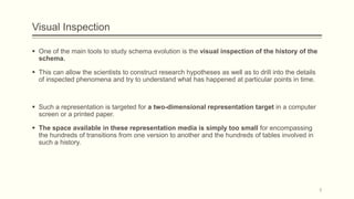
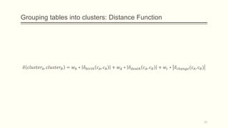
A dataset of schema transitions from the evolution history of the database of an AI assistant over 10 years. It contains 100 transitions. Wikipedia: A dataset of schema transitions from the evolution history of the database behind the Wikipedia website over 15 years. It contains 250 transitions. Hospital: A dataset of schema transitions from the evolution history of the database of a hospital information system over 7 years. It contains 50 transitions. 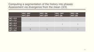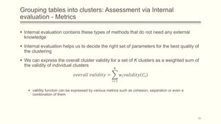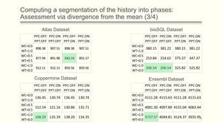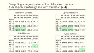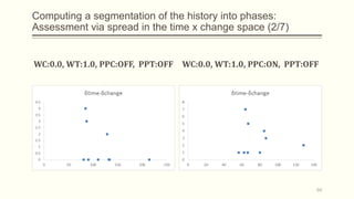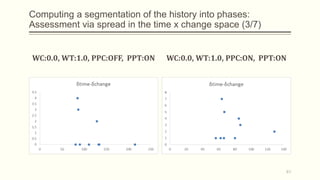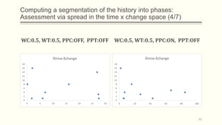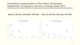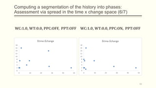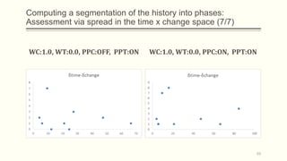For each dataset, we run Phasic Extractor for different values of k and we compute the divergence from the mean for each extracted phase. Lower values indicate better quality phases. We can observe that for k close to the “ground truth” number of phases: - Assistant: 3 phases

1. BIOGRAPHY SYNOPSES
FOR EVOLVING
RELATIONAL DATABASE
SCHEMATA
Theofanis Giachos
Supervisor: Panos Vassiliadis

2. Structure
 Introduction
 Problem Specification
 Creating an overview of the history of a schema
 Plutarch’s Parallel Lives Results
 Conclusions and Open Issues
2

3. Structure
 Introduction
 Problem Specification
 Creating an overview of the history of a schema
 Plutarch’s Parallel Lives Results
 Conclusions and Open Issues
3

4. General Facts
 Studying the evolution of database schemata is of great importance.
 A change in the schema of the database can impact the entire ecosystem of
applications that are built on top of the database.
 The study of schema evolution entails extracting schema versions and their delta
changes from software repositories, subsequently leading to the extraction of patterns
and regularities.
 The history of a typical database can consist of hundreds of transitions and includes a
potentially large number of tables.
4

5. Visual Inspection
 One of the main tools to study schema evolution is the visual inspection of the history of the
schema.
 This can allow the scientists to construct research hypotheses as well as to drill into the details
of inspected phenomena and try to understand what has happened at particular points in time.
 Such a representation is targeted for a two-dimensional representation target in a computer
screen or a printed paper.
 The space available in these representation media is simply too small for encompassing
the hundreds of transitions from one version to another and the hundreds of tables involved in
such a history.
5

6. Our Solution
 The main idea is the creation of a synopsis of the history of the schema evolution.
 The number of transitions is abstracted by a limited set of phases and the number of
tables is represented by a limited number of table clusters.
 Then, we can represent this synopsis as a 2D diagram, with the details of change in
the contents of this 2D space.
6

7. How we achieve our solution (1/2)
Phase Extraction
 We introduce a hierarchical agglomerative clustering algorithm that merges the most
similar transitions.
 As a result we can have a desired number of phases, each of which encompasses
subsequent and similar transitions.
Cluster Extraction
 We introduce another hierarchical agglomerative clustering algorithm that creates a
desired number of clusters.
 Within each cluster, the desideratum is to maximize the similarity of the contained
tables.
7

8. How we achieve our solution (2/2)
Plutarch’s Parallel Lives tool
Plutarch’s Parallel Lives (in short, PPL) tool combines our abovementioned
contribution and allows an interactive exploration of the history of schema.
Functionalities:
 Production of a detailed visualization of the life of the database, called Parallel Lives
Diagram
 Production of an overview for this visualization, which has the extracted phases in its
x-axis and the extracted clusters in its y-axis
 Zooming into specific points
 Filters according to specific criteria
 Details on demand
8

9. Terminology (1/2)
 Schema Version, or simply, Version: A snapshot of the database schema, committed
to the public repository that hosts the different versions of the system
 Dataset: A sequence of versions, respecting the order by which they appear in the
repository that hosts the project to which the database belongs
 Transition: The fact that the database schema has been migrated from version vi to
version vj, i < j
 Revision: A transition between two sequential versions, i.e., from version vi to version
vi+1
 History of a database schema: A sequence of revisions
9

10. Terminology (2/2)
For each transition, for each relation, we can identify the following data:
 Old Attributes: The set of attributes of the relation at the source, old version of the
transition
 New Attributes: The set of attributes of the relation at the target, new version of the
transition
 Attributes Inserted: The set of attribute names inserted in the relation in the new version
of the transition
 Attributes Deleted: The set of attribute names deleted from the relation during the
transition from the old to the new version
 Attributes with Type Alternations: The set of attributes whose data type changed during
a transition.
 Attributes involved in Key Alternations: The set of attributes that reversed their status
concerning their participation to the primary key of the relation between the old and the
new version of the transition
10

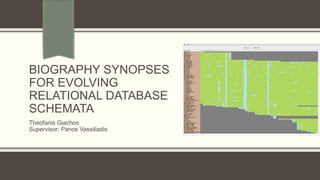
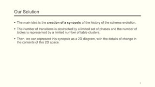
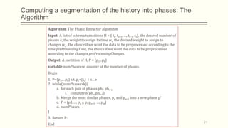
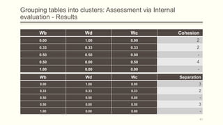
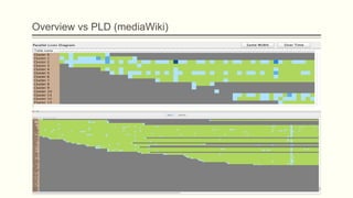
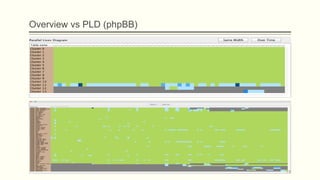
11. Visual representation of a history of a database (1/3)
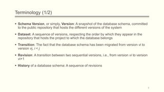
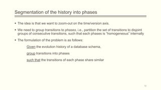
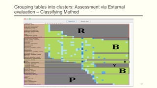
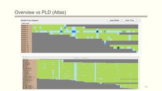
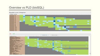
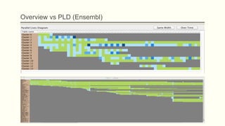
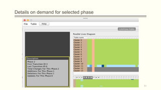
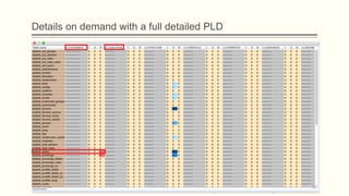
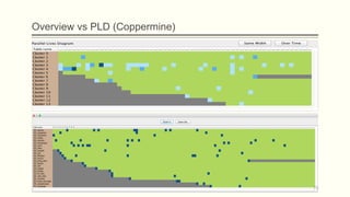
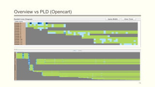
Parallel (Table) Lives Diagram of a database schema: a two dimensional rectilinear
grid having all the revisions of the schema’s history as columns and all the relations of
the diachronic schema as its rows
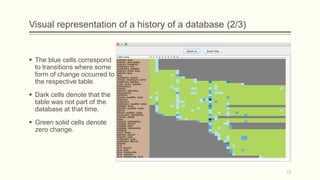
Each cell PLD[i,j] represents the changes undergone and the status of the relation at row
i during the revision j.
11

12. Visual representation of a history of a database (2/3)
 The blue cells correspond
to transitions where some
form of change occurred to
the respective table.
 Dark cells denote that the
table was not part of the
database at that time.
 Green solid cells denote
zero change.
12

13. Visual representation of a history of a database (3/3)
13

14. Structure
 Introduction
 Problem Specification
 Creating an overview of the history of a schema
 Plutarch’s Parallel Lives Results
 Conclusions and Open Issues
14

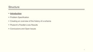
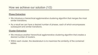
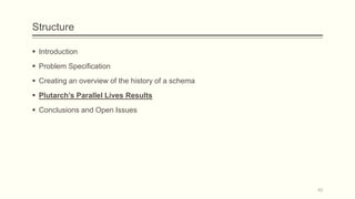
15. Intuition on the problem
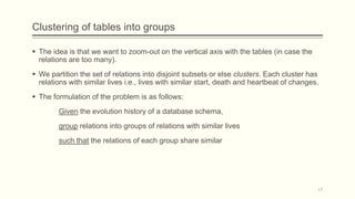
 The idea came from the mantra that Shneiderman underlines in his article at 1996
[Shne96], which is
Overview first, zoom and filter, details on demand.
15
Construct an
overview
instead of a
non-fitting
diagram

16. Segmentation of the history into phases
 The idea is that we want to zoom-out on the time/version axis.
 We need to group transitions to phases, i.e., partition the set of transitions to disjoint
groups of consecutive transitions, such that each phases is “homogeneous” internally
 The formulation of the problem is as follows:
Given the evolution history of a database schema,
group transitions into phases
such that the transitions of each phase share similar
16

17. Clustering of tables into groups
 The idea is that we want to zoom-out on the vertical axis with the tables (in case the
relations are too many).
 We partition the set of relations into disjoint subsets or else clusters. Each cluster has
relations with similar lives i.e., lives with similar start, death and heartbeat of changes.
 The formulation of the problem is as follows:
Given the evolution history of a database schema,
group relations into groups of relations with similar lives
such that the relations of each group share similar
17

18. Zoom, filter and details on demand
 Zoom into a specific point of the overview: if we have a matrix in which the x-axis
contains the phases and the y-axis contains the tables of the database or the clusters
how we could zoom into a specific cell of this table?
 Filter the overview: often there is the desire to isolate a component of an overview
including its elements to compare for example how similar are the elements from
which it consists of.
 Details on demand: if the PLD contains in its x-axis the phases and the clusters in its
y-axis what details we could get about a cell of PLD?
18

19. Structure
 Introduction
 Problem Specification
 Creating an overview of the history of a schema
 Plutarch’s Parallel Lives Results
 Conclusions and Open Issues
19

20. Creating an overview of the history of the database
Creation of an overview of the history of the database consists of two parts:
 Computing a segmentation of the history into phases
 Phase extraction algorithm (on the basis of a parameterized distance function)
 Assessment of the quality of result & parameter tuning
 Grouping tables into table clusters
 Table clustering algorithm (on the basis of a parameterized distance function)
 Assessment of the quality of result & parameter tuning
20

21. Computing a segmentation of the history into phases: The
Algorithm
Algorithm: The Phasic Extractor algorithm
Input: A list of schema transitions H = { ts, ts+1, …, te-1, te}, the desired number of
phases k, the weight to assign to time wt, the desired weight to assign to
changes wc , the choice if we want the data to be preprocessed according to the
time preProcessingTime, the choice if we want the data to be preprocessed
according to the changes preProcessingChanges.
Output: A partition of H, P = {p1...pk}
variable numPhases=e, counter of the number of phases.
Begin
1. P={p1,…pe} s.t. pi={ti} i s…e
2. while(numPhases>k){
a. for each pair of phases phi, phi+1,
i. compute δ(phi, phi+1)
b. Merge the most similar phases, pa and pa+1 into a new phase p’
c. P = {p1,…, pa-1, p, pa+1, …, pm}
d. numPhases --
}
3. Return P;
End
21

22. Computing a segmentation of the history into phases:
Parameters
 Desired number of segments (k): refers to the number of phases that we would like
to be extracted.
 Pre-Processing Changes (PPC): refers to the preprocessing of the data from the
aspect of changes (ON if the data has been preprocessed, OFF otherwise).
 Pre-Processing Time (PPT): refers to the preprocessing of the data from the aspect
of time (ON if the data has been preprocessed, OFF otherwise).
 Weight Change (WC): refers to the weight of changes (0.5 normal weight, 0 if
changes is not taken into account).
 Weight Time (WT): refers to the weight of time (0.5 normal weight, 0 if time is not
taken into account).
22

23. Computing a segmentation of the history into phases: Distance
Function
𝛿 𝑝𝑖, 𝑝𝑖+1 = 𝑤 𝑇
× 𝛿 𝑇
𝑝𝑖, 𝑝𝑖+1 + 𝑤 𝐶
× 𝛿 𝐶
(pi, p𝑖+1)
23

24. Computing a segmentation of the history into phases:
Assessment via divergence from the mean (1/3)
𝐸 𝑝𝑛 =
∀𝑝ℎ𝑎𝑠𝑒 𝑝ℎ 𝑖 ∀𝑒𝑣𝑒𝑛𝑡 𝑒 𝑗 ∈𝑝ℎ 𝑖
𝜇𝑖 − 𝑒𝑗
𝑝
1
𝑝
 μi is the average number of changes of each phase
 ej is the number of changes of each phase’s event
 Typically p is equal to one or two
24

25. Computing a segmentation of the history into phases:
Assessment via divergence from the mean (2/3)
Datasets that were used by Phasic Extractor
 Atlas
 bioSQL
 Coppermine
 Ensembl
 mediaWiki
 Opencart
 phpBB
 typo3
25

26. Computing a segmentation of the history into phases:
Assessment via divergence from the mean (3/3)
PPC: OFF
PPT: OFF
PPC: ON
PPT: OFF
PPC: OFF
PPT: ON
PPC: ON
PPT: ON
WC = 0.0
WT = 1.0
- - - -
WC = 0.5
WT = 0.5
- - 1 1
WC = 1.0
WT = 0.0
5 3 - 1
26

27. Computing a segmentation of the history into phases:
Assessment via spread in the time x change space (1/2)
The second assessment method can be described as follows:
For each pair of phases phi and phi+1 :
 compute the term δtime
 compute is the term δchange
 When these two terms have been computed for the whole set of pairs we can
represent our results with the scatter plot format.
27

28. Computing a segmentation of the history into phases:
Assessment via spread in the time x change space (2/2)
28
WC:0.0
WT:1.0
PPC:OFF
PPT:OFF
WC:0.0
WT:1.0
PPC:ON
PPT:OFF
WC:0.0
WT:1.0
PPC:OFF
PPT:ON
WC:0.0
WT:1.0
PPC:ON
PPT:ON
WC:0.5
WT:0.5
PPC:OFF
PPT:OFF
WC:0.5
WT:0.5
PPC:ON
PPT:OFF
WC:0.5
WT:0.5
PPC:OFF
PPT:ON
WC:0.5
WT:0.5
PPC:ON
PPT:ON
WC:1.0
WT:0.0
PPC:OFF
PPT:OFF
WC:1.0
WT:0.0
PPC:ON
PPT:OFF
WC:1.0
WT:0.0
PPC:OFF
PPT:ON
WC:1.0
WT:0.0
PPC:ON
PPT:ON

29. Grouping tables into clusters: The Algorithm
Algorithm: The Clustering Extractor algorithm
Input: The entire set of the database’s tables T {tab1, ... , tabn}, the desired number of
clusters k, the weight to assign to birth date wb, , the weight to assign to death date wd, ,
the weight to assign to heartbeat of the changes date wc
Output: A partition of T, C={c1, … , ck}
variable numClusters=n, counter of the number of clusters
Begin
1. C={c1, … , cn} s.t. ci = {tabi} i 1…n
2. while(numClusters>k){
a. for each pair of clusters ci, ci+1,
i. compute the δ(ci,ci+1)
b. Merge the most similar clusters, ca and ca+1 into a new cluster c’
c. C = {c1,…, ca-1, c, ca+1, …, cm}
d. numClusters –-
}
3. Return C;
End 29

30. Grouping tables into clusters: Parameters
 Desired number of clusters (k): refers to the number of clusters that we would like to
be created.
 Birth Weight (BW): refers to the weight of the distance between birth dates of
compared clusters.
 Death Weight (DW): refers to the weight of the distance between death dates of
compared clusters.
 Change Weight (CW): refers to the weight of the distance between the changes of
compared clusters.
30

31. Grouping tables into clusters: Distance Function
𝛿 𝑐𝑙𝑢𝑠𝑡𝑒𝑟𝐴, 𝑐𝑙𝑢𝑠𝑡𝑒𝑟𝐵 = 𝑤 𝑏 ∗ 𝛿 𝑏𝑖𝑟𝑡ℎ 𝑐 𝐴, 𝑐 𝐵 + 𝑤 𝑑 ∗ 𝛿 𝑑𝑒𝑎𝑡ℎ 𝑐 𝐴, 𝑐 𝐵 + 𝑤𝑐 ∗ 𝛿 𝑐ℎ𝑎𝑛𝑔𝑒(𝑐 𝐴, 𝑐 𝐵)
31

32. Grouping tables into clusters: Clustering Validity Techniques
There are two main categories for clustering validity:
 Internal evaluation: refers to methods that do not need external knowledge and can
measure the quality of the clusters only with the information that they keep and which
was used from the clustering algorithm
 External evaluation: needs external knowledge, i.e., data have to be classified before
the evaluation process, by explicit tracing of human knowledge on the issue.
32

33. Grouping tables into clusters: Assessment via External
evaluation - Metrics
There is a large amount of methods that have been used previously.
We decided to choose the most common of them
 Entropy: is defined as the degree to which each cluster consists of objects of a single
class.
For each cluster j we compute pij, which is the probability that a member of cluster i belongs
to class j.
𝑝𝑖𝑗 =
𝑚𝑖𝑗
𝑚𝑖
 mi is the number of objects in cluster i.
 mij is the number of objects of class j in cluster i.
The total entropy of each cluster i is calculated by the following formula:
𝑒𝑖 = −
𝑗=1
𝐿
𝑝𝑖𝑗 log2 𝑝𝑖𝑗
 L is the number of classes. 33

34. Grouping tables into clusters: Assessment via External
evaluation – Metrics
The total entropy of a set of clusters, is defined as the sum of the
entropies of each cluster weighted by the size of each cluster:
𝑒 =
𝑖=1
𝐾 𝑚𝑖
𝑚
𝑒𝑖
 K is the number of clusters and m is the total number of data points
 Precision: is defined as the fraction of a cluster that consists of objects of a
specified class. Precision of a cluster i with respect to class j is:
𝑝𝑟𝑒𝑐𝑖𝑠𝑖𝑜𝑛 𝑖, 𝑗 = 𝑝𝑖𝑗
34

35. Grouping tables into clusters: Assessment via External
evaluation - Metrics
 Recall: depicts the extent to which a cluster contains all the objects of a specified
class. The recall of cluster i with respect to class j is:
𝑟𝑒𝑐𝑎𝑙𝑙 𝑖, 𝑗 =
𝑚𝑖𝑗
𝑚𝑗
 mj is the number of objects in class j.
 F-measure: consists of both precision and recall and measures the extent to which a
cluster contains only objects of a particular class and all objects of that class.
The F-measure of cluster i with respect to class j is calculated by this formula:
𝐹 𝑖, 𝑗 =
2 × 𝑝𝑟𝑒𝑐𝑖𝑠𝑖𝑜𝑛 𝑖, 𝑗 × 𝑟𝑒𝑐𝑎𝑙𝑙 𝑖, 𝑗
𝑝𝑟𝑒𝑐𝑖𝑠𝑖𝑜𝑛 𝑖, 𝑗 + 𝑟𝑒𝑐𝑎𝑙𝑙 𝑖, 𝑗
35

36. Grouping tables into clusters: Assessment via External
evaluation – Classifying Method
 Datasets
 Atlas
 bioSQL
 Coppermine
 phpBB
 The source of our classification procedure was the PLD (Parallel Live Diagram).
 The most obvious criteria of the PLD are when a table is born (birth date) and when a
table died and not as much the count of changes of each table.
36

37. Grouping tables into clusters: Assessment via External
evaluation – Classifying Method
37

38. Grouping tables into clusters: Assessment via External
evaluation – Results
Average F-Measure Entropies
38
Parameters
Set
wb-wd-wc
Average
F-Measure
0.33 - 0.33 - 0.33 0.19
0.00 - 1.00 - 0.00 0.22
0.00 - 0.50 - 0.50 0.20
0.00 - 0.00 - 1.00 0.17
0.50 - 0.50 - 0.00 0.25
0.50 - 0.00 - 0.50 0.16
1.00 - 0.00 - 0.00 0.21
wb wd wc Entropy (e)
0.333 0.333 0.333 1.13
0 1 0 0.79
0 0.5 0.5 1.06
0 0 1 1.14
0.5 0.5 0 0.00
0.5 0 0.5 0.57
1 0 0 0.52

39. Grouping tables into clusters: Assessment via Internal
evaluation - Metrics
 Internal evaluation contains these types of methods that do not need any external
knowledge
 Internal evaluation helps us to decide the right set of parameters for the best quality of
the clustering
 We can express the overall cluster validity for a set of K clusters as a weighted sum of
the validity of individual clusters
𝑜𝑣𝑒𝑟𝑎𝑙𝑙 𝑣𝑎𝑙𝑖𝑑𝑖𝑡𝑦 =
𝑖=1
𝐾
𝑤𝑖 𝑣𝑎𝑙𝑖𝑑𝑖𝑡𝑦 𝐶𝑖
 validity function can be expressed by various metrics such as cohesion, separation or even a
combination of them
39

40. Grouping tables into clusters: Assessment via Internal
evaluation - Metrics
 Cohesion: can be defined as the sum of the proximities with respect to the prototype
(centroid or medoid) of the cluster
𝑐𝑜ℎ𝑒𝑠𝑖𝑜𝑛 𝐶𝑖 =
𝑥∈𝐶 𝑖
𝑝𝑟𝑜𝑥𝑖𝑚𝑖𝑡𝑦 𝑥, 𝑐𝑖 = 𝑑𝑖𝑠𝑡𝑎𝑛𝑐𝑒(𝑥, 𝑐𝑖)
 ci is the prototype of cluster Ci
 Separation of a cluster is defined as the proximity between the centroid ci of the cluster
and an overall centroid that has been calculated by the whole set of data points
𝑠𝑒𝑝𝑎𝑟𝑎𝑡𝑖𝑜𝑛 𝐶𝑖 = 𝑝𝑟𝑜𝑥𝑖𝑚𝑖𝑡𝑦 𝑐𝑖, 𝑐
 c is defined the overall centroid of the dataset
 We used the Euclidean distance as a measure of proximity.
40

41. Grouping tables into clusters: Assessment via Internal
evaluation - Results
Wb Wd Wc Cohesion
0.00 1.00 0.00 2
0.33 0.33 0.33 2
0.50 0.50 0.00 -
0.50 0.00 0.50 4
1.00 0.00 0.00 -
41
Wb Wd Wc Separation
0.00 1.00 0.00 3
0.33 0.33 0.33 2
0.50 0.50 0.00 -
0.50 0.00 0.50 3
1.00 0.00 0.00 -

42. Structure
 Introduction
 Problem Specification
 Creating an overview of the history of a schema
 Plutarch’s Parallel Lives Results
 Conclusions and Open Issues
42

43. Overview vs PLD (Atlas)
43

44. Overview vs PLD (bioSQL)
44

45. Overview vs PLD (Ensembl)
45

46. Zoom into a specific point of overview: PLD phases x tables
46

47. Zoom into a specific point of overview: PLD phases x clusters
47

48. Filter the overview of the history: Filter by a specific phase
48

49. Filter the overview of the history: Filter by a specific table
49

50. Filter the overview of the history: Filter by specific clusters
50

51. Details on demand for selected phase
51

52. Details on demand with a full detailed PLD
52

53. Structure
 Introduction
 Problem Specification
 Creating an overview of the history of a schema
 Results
 Conclusions and Open Issues
53

54. Conclusions
Conclusions:
 Creation of an interactive overview from the entire life of a database
 Phase Extraction Algorithm
 Cluster Extraction Algorithm
 Assessment of both of them
 Plutarch’s Parallel Lives tool
54

55. Open Issues
Open Issues
 Implementation of different distance metrics for phase extraction
 Implementation of different distance metrics for cluster extraction
 Enrichment of PPL with more features
55

56. Thank you!
56

57. Phase Extraction Distance Function Notations
57

58. Computing a segmentation of the history into phases:
Assessment via divergence from the mean (3/4)
PPC:OFF
PPT:OFF
PPC:ON
PPT:OFF
PPC:OFF
PPT:ON
PPC:ON
PPT:ON
WC=0.0
WT=1.0
898.38 907.51 898.38 907.51
WC=0.5
WT=0.5
877.94 891.98 840.24 855.17
WC=1.0
WT=0.0
912.11 912.11 859.56 859.56
PPC:OFF
PPT:OFF
PPC:ON
PPT:OFF
PPC:OFF
PPT:ON
PPC:ON
PPT:ON
WC=0.0
WT=1.0
380.15 381.22 380.15 381.22
WC=0.5
WT=0.5
253.84 254.62 375.37 347.37
WC=1.0
WT=0.0
206.54 206.54 325.82 325.82
Atlas Dataset bioSQL Dataset
Coppermine Dataset
PPC:OFF
PPT:OFF
PPC:ON
PPT:OFF
PPC:OFF
PPT:ON
PPC:ON
PPT:ON
WC=0.0
WT=1.0
136.45 130.74 136.45 130.74
WC=0.5
WT=0.5
112.54 121.16 130.86 135.71
WC=1.0
WT=0.0
108.29 135.39 138.20 134.35
Ensembl Dataset
PPC:OFF
PPT:OFF
PPC:ON
PPT:OFF
PPC:OFF
PPT:ON
PPC:ON
PPT:ON
WC=0.0
WT=1.0
4111.28 4115.63 4111.28 4115.63
WC=0.5
WT=0.5
4081.30 4097.89 4155.04 4083.44
WC=1.0
WT=0.0
3737.57 4044.81 4124.37 3935.9558

59. Computing a segmentation of the history into phases:
Assessment via divergence from the mean (4/4)
mediaWiki Dataset Opencart Dataset
phpBB Dataset typo3 Dataset
PPC:OFF
PPT:OFF
PPC:ON
PPT:OFF
PPC:OFF
PPT:ON
PPC:ON
PPT:ON
WC=0.0
WT=1.0 1052.28 1052.28 1052.28 1052.28
WC=0.5
WT=0.5 1025.91 1042.27 1030.86 1053.47
WC=1.0
WT=0.0 920.34 920.34 1061.43 1047.30
PPC:OFF
PPT:OFF
PPC:ON
PPT:OFF
PPC:OFF
PPT:ON
PPC:ON
PPT:ON
WC=0.0
WT=1.0 3390.19 3381.58 3390.19 3381.58
WC=0.5
WT=0.5 1297.10 1294.76 2733.91 2731.19
WC=1.0
WT=0.0 837.30 837.30 2745.29 2743.91
PPC:OFF
PPT:OFF
PPC:ON
PPT:OFF
PPC:OFF
PPT:ON
PPC:ON
PPT:ON
WC=0.0
WT=1.0 870.53 880.23 870.53 880.23
WC=0.5
WT=0.5 861.10 941.45 853.23 791.49
WC=1.0
WT=0.0 843.11 843.11 953.27 872.68
PPC:OFF
PPT:OFF
PPC:ON
PPT:OFF
PPC:OFF
PPT:ON
PPC:ON
PPT:ON
WC=0.0
WT=1.0 648.59 644.33 648.59 644.33
WC=0.5
WT=0.5 658.19 664.04 664.39 485.49
WC=1.0
WT=0.0 486.84 486.84 477.48 438.3559

60. Computing a segmentation of the history into phases:
Assessment via spread in the time x change space (2/7)
WC:0.0, WT:1.0, PPC:OFF, PPT:OFF WC:0.0, WT:1.0, PPC:ON, PPT:OFF
60

61. Computing a segmentation of the history into phases:
Assessment via spread in the time x change space (3/7)
WC:0.0, WT:1.0, PPC:OFF, PPT:ON WC:0.0, WT:1.0, PPC:ON, PPT:ON
61

62. Computing a segmentation of the history into phases:
Assessment via spread in the time x change space (4/7)
WC:0.5, WT:0.5, PPC:OFF, PPT:OFF WC:0.5, WT:0.5, PPC:ON, PPT:OFF
62

63. Computing a segmentation of the history into phases:
Assessment via spread in the time x change space (5/7)
WC:0.5, WT:0.5, PPC:OFF, PPT:ON WC:0.5, WT:0.5, PPC:ON, PPT:ON
63

64. Computing a segmentation of the history into phases:
Assessment via spread in the time x change space (6/7)
WC:1.0, WT:0.0, PPC:OFF, PPT:OFF WC:1.0, WT:0.0, PPC:ON, PPT:OFF
64

65. Computing a segmentation of the history into phases:
Assessment via spread in the time x change space (7/7)
WC:1.0, WT:0.0, PPC:OFF, PPT:ON WC:1.0, WT:0.0, PPC:ON, PPT:ON
65

66. Term Description Formula
𝛿(𝑐𝑙𝑢𝑠𝑡𝑒𝑟𝐴
, 𝑐𝑙𝑢𝑠𝑡𝑒𝑟𝐵
) Total distance between two clusters
𝑤𝑏
The weight that will be assigned to the
distance that is related with the birth date
𝛿 𝑏𝑖𝑟𝑡ℎ(𝑐 𝐴, 𝑐 𝐵) The distance between birth dates of the two
compared clusters
Plain
𝑐 𝐴. 𝑏𝑖𝑟𝑡ℎ − 𝑐 𝐵. 𝑏𝑖𝑟𝑡ℎ
Normalized
𝛿 𝑏𝑖𝑟𝑡ℎ 𝑐 𝐴, 𝑐 𝐵
𝐷𝐵 𝑑𝑢𝑟𝑎𝑡𝑖𝑜𝑛
𝑤 𝑑 The weight that will be assigned to the
distance that is related with the death date
𝛿 𝑑𝑒𝑎𝑡ℎ(𝑐 𝐴, 𝑐 𝐵) The distance between death dates of the two
compared clusters
Plain
∅, 𝒊𝒇 𝒃𝒐𝒕𝒉 𝒂𝒍𝒊𝒗𝒆
𝑐 𝐴. 𝑑𝑒𝑎𝑡ℎ − 𝑐 𝐵. 𝑑𝑒𝑎𝑡ℎ, 𝒆𝒍𝒔𝒆
Normalized
𝛿 𝑑𝑒𝑎𝑡ℎ 𝑐 𝐴, 𝑐 𝐵
𝐷𝐵 𝑑𝑢𝑟𝑎𝑡𝑖𝑜𝑛
𝑤𝑐
The weight that will be assigned to the
distance that is related with the total changes
𝛿𝑐ℎ𝑎𝑛𝑔𝑒(𝑐 𝐴, 𝑐 𝐵) The distance between the total changes that
have been committed to the two compared
clusters
Plain
𝑐 𝐴. 𝑐ℎ𝑎𝑛𝑔𝑒𝑠 − 𝑐 𝐵 𝑐ℎ𝑎𝑛𝑔𝑒𝑠
Normalized
𝐶ℎ(𝐴) − 𝐶ℎ(𝐵)
𝐶ℎ(𝐴) + 𝐶ℎ(𝐵)
where Ch is the total number
of changes
66

67. Grouping tables into clusters: Assessment via External
evaluation – Results
Atlas bioSQL
wb wd wc Entropy (e)
0.333 0.333 0.333 1.13
0 1 0 0.79
0 0.5 0.5 1.06
0 0 1 1.14
0.5 0.5 0 0.00
0.5 0 0.5 0.57
1 0 0 0.52
wb wd wc Entropy (e)
0.333 0.333 0.333 0.40
0 1 0 0.45
0 0.5 0.5 0.51
0 0 1 1.14
0.5 0.5 0 0.32
0.5 0 0.5 0.50
1 0 0 0.30
67

68. Grouping tables into clusters: Assessment via External
evaluation – Results
Coppermine phpBB
wb wd wc Entropy (e)
0.333 0.333 0.333 0.13
0 1 0 0.94
0 0.5 0.5 0.28
0 0 1 0.28
0.5 0.5 0 0.00
0.5 0 0.5 0.20
1 0 0 0.26
wb wd wc Entropy (e)
0.333 0.333 0.333 0.38
0 1 0 0.19
0 0.5 0.5 0.38
0 0 1 0.38
0.5 0.5 0 0.19
0.5 0 0.5 0.60
1 0 0 0.00
68

69. Grouping tables into clusters: Assessment via Internal
evaluation - Results
Atlas
Wb Wd Wc Cohesion Separation
0.00 1.00 0.00 1323.69 2115.12
0.33 0.33 0.33 650.45 2598.62
0.50 0.50 0.00 331.31 2797.45
0.50 0.00 0.50 1383.74 2049.81
1.00 0.00 0.00 1271.30 2314.82
Coppermine
Wb Wd Wc Cohesion Separation
0.00 1.00 0.00 211.33 362.10
0.33 0.33 0.33 35.62 421.41
0.50 0.50 0.00 40.16 418.65
0.50 0.00 0.50 35.62 421.41
1.00 0.00 0.00 40.16 418.65 69

70. Grouping tables into clusters: Assessment via Internal
evaluation - Results
bioSQL
Wb Wd Wc Cohesion Separation
0.00 1.00 0.00 320.45 781.45
0.33 0.33 0.33 159.73 890.94
0.50 0.50 0.00 122.00 886.21
0.50 0.00 0.50 473.46 668.98
1.00 0.00 0.00 253.59 827.05
Ensembl
Wb Wd Wc Cohesion Separation
0.00 1.00 0.00 11167.50 30780.37
0.33 0.33 0.33 21301.49 21566.66
0.50 0.50 0.00 5289.72 33661.45
0.50 0.00 0.50 19684.44 24562.84
1.00 0.00 0.00 14182.14 27347.17 70

71. Grouping tables into clusters: Assessment via Internal
evaluation - Results
mwiki
Wb Wd Wc Cohesion Separation
0.00 1.00 0.00 4653.55 6882.07
0.33 0.33 0.33 1752.76 9397.74
0.50 0.50 0.00 1033.57 9561.50
0.50 0.00 0.50 5349.92 7390.00
1.00 0.00 0.00 4775.46 7740.74
Opencart
Wb Wd Wc Cohesion Separation
0.00 1.00 0.00 3924.06 15890.54
0.33 0.33 0.33 3359.07 16089.72
0.50 0.50 0.00 2366.92 16189.32
0.50 0.00 0.50 7604.85 13317.76
1.00 0.00 0.00 3202.38 16068.17 71

72. Grouping tables into clusters: Assessment via Internal
evaluation - Results
phpBB
Wb Wd Wc Cohesion Separation
0.00 1.00 0.00 766.54 2053.20
0.33 0.33 0.33 2243.29 512.37
0.50 0.50 0.00 506.25 2196.72
0.50 0.00 0.50 2104.33 565.81
1.00 0.00 0.00 506.25 2196.72
typo3
Wb Wd Wc Cohesion Separation
0.00 1.00 0.00 414.14 1096.70
0.33 0.33 0.33 192.07 1240.47
0.50 0.50 0.00 239.91 1213.34
0.50 0.00 0.50 208.57 1212.90
1.00 0.00 0.00 277.97 1200.29 72

73. Overview vs PLD (Coppermine)
73

74. Overview vs PLD (Opencart)
74

75. Overview vs PLD (mediaWiki)
75

76. Overview vs PLD (phpBB)
76

77. Details on demand for selected cluster
77

78. Details on demand for selected cell
78

79. References
[ECLI15] Eclipse IDE. Available at https://eclipse.org/downloads/. Last accessed 2015-09-30.
[HECA15] Hecate. Available at https://github.com/daintiness-group/hecate . Last accessed 2015-09-30.
[PPL15] Plutarch’s Parallel Lives at https://github.com/daintiness-group/plutarch_parallel_lives. Last
accessed 2015-09-30
[Shne96] Shneiderman, Ben. "The eyes have it: A task by data type taxonomy for information
visualizations." Visual Languages, 1996. Proceedings., IEEE Symposium on. IEEE, 1996.
[SkVZ14] Skoulis, Ioannis, Panos Vassiliadis, and Apostolos Zarras. "Open-Source Databases: Within,
Outside, or Beyond Lehman’s Laws of Software Evolution?."Advanced Information Systems
Engineering. Springer International Publishing, 2014.
[TaSK05] Pang-Ning Tan, Michael Steinbach and Vipin Kumar. Introduction to Data Mining. 1st ed.
Pearson, 2005.
[TaTT06] Mielikäinen, Taneli, Evimaria Terzi, and Panayiotis Tsaparas. "Aggregating time
partitions." Proceedings of the 12th ACM SIGKDD international conference on Knowledge
discovery and data mining. ACM, 2006.
[TeTs06] Terzi, Evimaria, and Panayiotis Tsaparas. "Efficient Algorithms for Sequence
Segmentation." SDM. 2006.
[ZhSt05] Xing, Zhenchang, and Eleni Stroulia. "Analyzing the evolutionary history of the logical design
of object-oriented software." Software Engineering, IEEE Transactions on 31.10 (2005): 850-
868.
79