BIM-Integrated predictive model for schedule delays in Construction

A BIM-INTEGRATED FRAMEWORK TO PREDICT SCHEDULE DELAYS IN
MODULAR CONSTRUCTION
By
SAHIL NAVLANI
A Plan B Report
Submitted to
Michigan State University
in partial fulfillment of the requirements
for the degree of
Construction Management – Master of Science
2017/04

ii
ABSTRACT
A BIM-INTEGRATED FRAMEWORK TO PREDICT SCHEDULE DELAYS IN
MODULAR CONSTRUCTION
BY
SAHIL NAVLANI
“Information is the oil of the 21st
century, and analytics is the combustion engine” are thought-
provoking words by the Gartner Research’s, Peter Sondergaard. Literature has provided
qualitative classification, management and mitigation techniques on scheduling risk in
construction projects; however, it has not shed light on quantitative techniques on schedule risk
management at a micro-level. Therefore, the construction industry has been encountering
critical issues in project delays. Fortunately, technological advances, such as the building
information modeling (BIM), offer potential solutions.
This report aims to establish a BIM-integrated framework that can be used to provide data-
driven scheduling decisions for construction management. The study explores the intersection
of the construction and data analytics domains. The framework captures operational data from
a BIM model and put them into a machine learning algorithm to facilitate prediction. This study
adopts the CRISP-Data Mining model in data structuring and data warehousing to facilitate
machine learning. The study’s methodological strategy is aligned with the LEAN six sigma
process improvement cycle, which can define data by structuring, measure data by schedule
variations, analyzes data on the delay causes, improves performance through delay prediction,
and control through demonstration. Outcomes from this study provide an analytical tool that
enables to predict scheduling delays using BIM models, particularly for modular construction.

iii
“My research is dedicated to my mom and dad, who have provided me with
the ethics morals and values to become the person I’m today”

iv
ACKNOWLEDGEMENTS
This research is an outcome of the collective effort of people who have motivated, encouraged,
enlightened me in many ways. I would like to identify and offer gratitude to some of the key
players to this result.
I would like to thank Dr. Dong Zhao, for believing in me and introducing me to the wonderful
world of research. Dr. Zhao has encouraged and guided me in professional and personal
pursuits. Without his confidence in me, I wouldn’t have come this far. I’d also like to thank Dr.
Berghorn for joining forces and being on my committee.
I’m grateful to Prof. Matt Syal, for the enormous ways he has refined me. I admire him for his
energy and enthusiasm towards education. I also want to acknowledge Dr. Tariq Abdelhamid
for fostering a great learning environment and the amazing human being he is.
I’d like to conclude by thanking all friends and family for standing together through all the
highs and lows, bringing out the best in me.

v
TABLE OF CONTENTS
ABSTRACT...............................................................................................................................ii
ACKNOWLEDGEMENTS......................................................................................................iv
TABLE OF CONTENTS...........................................................................................................v
LIST OF TABLES..................................................................................................................viii
LIST OF FIGURES ..................................................................................................................ix
CHAPTER 1 INTRODUCTION ..............................................................................................1
1.1. Overview.....................................................................................................................1
1.2. Problem Statement ......................................................................................................1
1.3. Research Objectives ....................................................................................................3
1.4. Research Scope ...........................................................................................................4
1.5. Research strategy.........................................................................................................5
CHAPTER 2 LITERATURE REVIEW ....................................................................................9
2.1. Introduction.................................................................................................................9
2.2. Background of Project Risk Management ..................................................................9
2.3. Risk Management Process ........................................................................................10
2.3.1. Risk Identification..............................................................................................11
2.3.2. Risk Assessment/Analysis .................................................................................12
2.3.3. Risk responses....................................................................................................13
2.3.4. Risk Control.......................................................................................................15
2.4. Project Risk Assessment and Allocation...................................................................15
2.5. Schedule Risk Management......................................................................................17

vi
2.6. Data Analytics in Construction .................................................................................22
2.7. Manufactured and Modular Housing ........................................................................24
2.8. Chapter Summary......................................................................................................25
CHAPTER 3 METHODOLOGY ............................................................................................27
3.1. Overview...................................................................................................................27
3.2. Data Diagnosis ..........................................................................................................28
3.3. Data Structuring ........................................................................................................32
3.4. Data Warehousing.....................................................................................................34
3.5. Predictive Modeling..................................................................................................35
CHAPTER 4 FRAMEWORK DEVELOPMENT...................................................................39
4.1.1 Identification of Instance-Attribute level...........................................................42
4.3.1. Feature Engineering...........................................................................................47
4.3.2. Algorithms for Predictive Modeling..................................................................47
CHAPTER 5 FRAMEWORK DEMONSTRATION.............................................................51
5.1. Case introduction.......................................................................................................51
5.4.1. Feature Engineering...........................................................................................58

vii
5.4.2. Classification Algorithm....................................................................................59
5.5. Summary and Interpretation of Results.....................................................................61
CHAPTER 6 CONCLUSION.................................................................................................64
6.1. Research Outcomes...................................................................................................64
6.2. Limitations ................................................................................................................65
6.3. Future Research.........................................................................................................65
6.4. Concluding Remarks.................................................................................................65
Appendices...............................................................................................................................67
Appendix A: Excel Macro Code..........................................................................................67
Appendix B: Weka Model Output .......................................................................................80
References................................................................................................................................82

viii
LIST OF TABLES
Table 1. Various risk analysis techniques (Ward & Chapman, 1997).....................................13
Table 2. Level of Development Schema (BIMForum, 2016)..................................................40

ix
LIST OF FIGURES
Figure 1. Lean Six Sigma DMAIC process flow (Forbes & Ahmed, 2011) .............................6
Figure 2. CRISP-DM Process flow (Wirth & Hipp, 2000)........................................................7
Figure 3. Superimposed DMAIC and CRISP-DM process flow...............................................8
Figure 4. Approach to Risk Management in Construction ......................................................10
Figure 5. Scope of Risk Management (Project Management Institute, 2016).........................11
Figure 6. Risk Breakdown Structure (El-Sayegh, 2008) .........................................................16
Figure 7. Research Methodology.............................................................................................27
Figure 8. Knowledge base information flow diagram .............................................................28
Figure 9. Critical path method example...................................................................................31
Figure 10. Data transformation from structuring to warehousing ...........................................34
Figure 11. Analytics and related fields ....................................................................................36
Figure 12. Framework workflow .............................................................................................39
Figure 13. Project & shared parameter management in Autodesk Revit.................................42
Figure 14. IFC file ontology ....................................................................................................43
Figure 15. Modular house model authored in Revit ................................................................52
Figure 16. Case Demonstration data-flow eliciting the tools used..........................................53
Figure 17. Schedule parameters created using project parameters..........................................55
Figure 18. Corresponding IFC export file depicting the created parameters...........................55
Figure 19. Interface of Simplebim 6........................................................................................56
Figure 20. VBA enabled excel sheet........................................................................................57
Figure 21. WEKA explorer interface with data distribution visualization..............................58

x
Figure 22. Feature Engineering and distribution of the attributes ...........................................59
Figure 23. Linear regression as the classification algorithm ...................................................60
Figure 24. Simulating the test options for model training .......................................................61
Figure 25. Predictive modeling results ....................................................................................62
Figure 26. Scatter plot for the predicted vs actual values........................................................63

1
CHAPTER 1
INTRODUCTION
1.1. Overview
Risk management is a salient knowledge area in project risk management. Recent studies have
broadly classified risks in a construction project as internal risks; which falls within the control
of clients, consultants and contractors, and external risks; which include risk elements that are
not in control of key stakeholders (Banaitiene & Banaitis, 2012; El-Sayegh, 2008; Chapman &
Ward, 1997). Project management risks were among the top internal risks category. Scheduling
errors and contractor delays were most likely to happen and had a high impact on the project.
A national survey of owners by Construction Managers Association of America (FMI
Corporation, 2007) indicated that 40-50% of all major construction projects run longer than
planned and incur significant cost overruns. Building Information Modeling (BIM) has been
demonstrated to substantially improve the information environment for the construction risk
identification and prevention of scheduling errors and delays.
1.2. Problem Statement
Risk management is one of the ten project management knowledge areas: Integration
management, Scope management, Time management, Cost management, Quality
management, Human Resource management, and Communication management, under the
Project Management Book of Knowledge (PMBOK) by the Project Management Institute
(PMI). Risk management knowledge comprises of the planning, identification, analyzing,

2
responding and controlling processes. Scheduling errors and contractor delays have been
categorized as some of the most frequent and impactful project management risks (Banaitiene
& Banaitis, 2012). The construction industry is perceived to be highly risk-prone and possesses
poor risk coping skills as many projects fail to meet timelines and cost targets (Zavadskas,
Turskis, & Tamosaitiene, 2010; Shevchenko, Ustinovichius, & Andruskevicius, 2008). Major
risk management techniques and practices have been identified, quantified and modeled the
relationships between risk variables to perform Monte Carlo simulation for predicting delays
in a building construction project (Iqbal, Choudhry, Holschemacher, Ali, & Tamosaitiene,
2015; Nasir, McCabe, & Hartono, 2003). Although the framework has demonstrated to give
out results within an acceptable margin of error, the fact that the experts took six weeks to
respond to the risk identification matrix.
Research is needed to reuse the knowledge base gained through operations and to statistically
model the schedule delays from the knowledge base to support data-driven decisions. Risk
management on construction projects is implemented through contracts, insurances, and expert
judgments. A majority of risk mitigation practices rely on expert judgments. Implementation
of risk management in construction has been managed through BIM using semantic
relationships (Ding, Zhong, Wu, & Luo, 2016). The literature reflects the gap in mitigating the
risks quantitatively. Some of the new contractual delivery methods, such as Integrated Project
Delivery (IPD), help in managing risk by involving the stakeholders in a common risk pool.

3
1.3. Research Objectives
The goal of this research is to develop and demonstrate a BIM-integrated framework to predict
construction delays, especially for modular construction projects. The practical target of this
research is to provide with a feasible framework to reuse the documented operational
knowledge. Results from this study contribute to the knowledge in construction projects for
scheduling risk management, listed as follows:
• Data analytics methods in the construction operations domain for risk mitigation.
• Data-driven prediction workflows on a construction project schedule.
• Schedule risk identification on construction projects in a timely manner.
Specific objectives of the study are as follows:
• Research Objective 1: Define the data structure of Virtual Design and Construction
(VDC) technology to streamline operational workflow for project risk knowledge
management.
• Research Objective 2: Develop an analytic framework to predict schedule data for data-
driven assistance to facilitate construction schedule decision making.
• Research Objective 3: Demonstrate the framework through a case study.
The main research question that guides this research are as follows:

4
“Statistical data from construction has suggested of most construction projects to be behind
schedule and/or over budget primarily due to delayed schedule. Can schedule delays be
predicted and mitigated quantitatively on a project? If so, how?”
1.4. Research Scope
The research aims at providing a framework to enable knowledge reuse on construction
projects. The knowledge reuse has twofold results- Data driven decisions on a project, realistic
schedule monitoring. The proposed framework is comprised of tools from VDC and data
analytics domains. The scope of the research is:
• To blend data warehousing techniques with BIM outlining the data structure.
• To compare as-built data with as-planned data, tracking anomalies adding to the
knowledge base.
Using the knowledge base to perform predictive analytics on current datasets employing linear
regression, to accomplish the end-goal of quantitatively reusing the qualitative knowledge. This
research compares as-built models with as-planned models to track anomalies. The scope of
the research has been limited to internal project management risks in forms of construction
delays due to sub-contractor delays, procurement delays. The research performs analytics on
the specific attributes of the datasets shown to be of highest impact by the literature and the
author’s analysis. The datasets are structured to activity levels defined in the schedules and
their respective attributes.

5
For the demonstration part of the study, a specialty construction setting is considered, with a
highly experienced modular construction company serving the residential housing building
industry. BIM models and conceptual schedules are to be considered from the built
environment for a demonstration of the framework.
1.5. Research strategy
The research study is based on the lean six sigma “DMAIC” cycle, refer figure 1. The author
found a need for process improvement in the project risk management knowledge area, as also
reflected in the literature review. Lean six sigma is simply a process for solving a problem. It
consists of five basic phases: Define, Measure, Analyze, Improve and Control (Forbes &
Ahmed, 2011). The selected research problem in the construction planning domain has an
obvious problem within the process, has potential to result in increased revenue, reduced cost
or improved efficiency and has collectible data. The DMAIC process follows the flow as:
• Define. Understand the problem
• Measure. Quantify the problem
• Analyze. Identify the cause of the problem.
• Improve. Implement and verify the solution.
• Control. Maintain the solution.

6
Figure 1. Lean Six Sigma DMAIC process flow (Forbes & Ahmed, 2011)
The study implements the tools and techniques used under the DMAIC process improvement
framework. Under the Define phase, the problem statement and scope is defined, which
corresponds to the Introduction chapter of this work. The Methodology chapter corresponds to
the Measure phase of process improvement, outlining the measures and data collection
techniques. The datasets will be analyzed by creating data warehouses to compare the as-built
data over as-planned data. Improvement phase is carried out by deploying Predictive analytics
to make data-driven predictions on a project backed by the knowledge base. The control phase
of the DMAIC cycle will be accomplished by validating the framework to document the
improvement process.

7
Figure 2. CRISP-DM Process flow (Wirth & Hipp, 2000)
The approach to data handling in the study is based upon CRISP-DM shown in Figure 2, which
stands for a Cross-industry process for data mining. It provides a structured approach to
planning a data mining project (North, 2012). The CRISP-DM model has further been defined
into phases as Business Understanding, Data Understanding, Data Preparation, Data Modeling,
Evaluation and Deployment. The resultant framework blends the Define phase of DMAIC
process with the Business and Data understanding phase of CRISP-DM, Measure with data
preparation which results into a data warehouse to be measured, Analyze and Improve phase
overlaps with the Modeling and Evaluation stage of CRISP-DM where predictive analytics is

8
used as a modeling technique to assess and evaluate the model. The Control and Deployment
stages blend into document deployment plan and experience. Figure 3 below shows the
DMAIC cycle superimposed on the CRISP-DM process.
DEFINE MEASURE ANALYZE IMPROVE CONTROL
Business & Data Data Data
Understanding Preparation Modeling Evaluation Deployment
• What Data is
available?
• What Data is
needed?
•What data is
important
beneficial to
Project Risk
management?
• Data stored
according to the
prescribed data
structure.
• Preparation of
Data Warehouse.
• Discovery of
hidden trends in
the prepared
datasets.
• Perform
predictive
modeling on the
prepared
datasets.
• Application of
data analytic
algorithms.
• Mapping the
outcomes for
further
qualitative input
to the schedule.
Figure 3. Superimposed DMAIC and CRISP-DM process flow

9
CHAPTER 2
LITERATURE REVIEW
2.1. Introduction
This chapter presents the background on project risk management knowledge area. Through
this literature review, the author provides an in-depth study of the prevailing Project risk
management and mitigation techniques in the Architecture, Engineering, and Construction
(AEC) industry. This chapter uses literature to classify project risk and elicits the previous
efforts by researchers to project risk management and mitigation. The author concludes the
literature review by acknowledging the gap in project risk management knowledge area and
illustrating how this research aims to fill the gap.
2.2. Background of Project Risk Management
According to the PMBOK 5th
Edition a project can be defined as a temporary endeavor
undertaken to create a unique product or service, in a specific timeline and risk can be defined
as an uncertain event or condition that, if it occurs, has a positive or negative effect on one or
more project objectives such as scope, schedule, cost or quality. Risk management is the
identification, assessment, and prioritization of risks followed by coordinated and economical
application of resources to minimize, monitor, and control the probability and/or impact of
unfortunate events or to maximize the realization of opportunities. Project risk management is
an important aspect of project management and is one of the ten knowledge areas defined in
the PMBOK. The PMBOK 5th
edition contains five processes specific to Project risk

10
management knowledge area as in plan risk management, identify risks, perform qualitative
risk analysis, perform quantitative risk analysis, plan risk responses and control risks. The
majority of risks on AEC projects are managed contractually and by insurances. According to
the American Institute of Constructors, Associate Constructor Certification study guide, the
contractor is expected to pay 9 dollars for every 1 dollar paid by the insurance. Figure 4 outlines
the prevailing approaches to risk management in construction while contrasting them over the
proposed framework.
Risk Management in Construction
Identify Analyze Respond
Qualitative & Evaluate
Surveys Based on Cost & Schedule
Analysis Experience Resource Constraints
Experience Cost Implications
Schedule Implications
Gut-Feeling
Knowledge Data Analysis Data-Driven Decisions
Base & Analytics Expert Judgement
2.3. Risk Management Process
Risk management in the construction industry is the assessment and response to the risk that
will be inevitably attached to a project (Simu, 2006). Risk management can be defined as the
practice of controlling occurrences that may result in a risk, instead of being passive before
such occurrences and reacting later (Renault & Agumba, 2016). The increasing complexity,
`
Proposed Framework
Figure 4. Approach to Risk Management in Construction

11
size, magnitude, client-consumer requirements and major physical conditions necessitate the
need for risk management on a construction project. The scope of risk management with
reference to PMI is shown in figure 5.
Figure 5. Scope of Risk Management (Project Management Institute, 2016)
2.3.1. Risk Identification
Risk Identification is the preliminary phase of capturing all possible, tangible risks/effects. Risk
Identification lays the foundation of Risk management and aligns the process. Appropriate
application of risk identification to supplement the risk management process, as unknown
sources of losses, escalate into unmanageable occurrences with unforeseen outcomes, has been
identified and addresses the effect of the non-identification of positive risks equating to the
effect of non-identification of negative risks (Haugan, 2002). The PMBOK 5th
Edition has
identified documentation reviews, information gathering techniques, checklist analysis,

12
assumption analysis, diagramming techniques, Strength-Weakness-Opportunity-Threat
analysis, and expert judgment as the tools and techniques in the process of risk identification
The best-known tools and techniques in the AEC industry are brainstorming, interviews,
questionnaires, Delphi technique, and expert systems. The documentation review is carried
upon the project charter, scope statement and the project management plan including the work
breakdown structure and schedule.
2.3.2. Risk Assessment/Analysis
Upon comprehensive identification of risks, risk assessment/analysis is performed in the
process of project risk management. Risk assessment has been stated to be a method of using
available information for determination of the frequency of occurrence and the level of
consequences in risk management (Olamiwale, 2014). The PMBOK 5th
edition further
subdivides this step into qualitative and quantitative risk analysis, as in table 1. The qualitative
risk analysis classifies risks on basis of priority and quantitative risk analysis examines the cost,
time, quality effects of the prioritized qualitative risks.

13
Table 1. Various risk analysis techniques (Ward & Chapman, 1997)
Risk Analysis
Qualitative Quantitative
Direct Judgement Probability analysis
Ranking options Sensitivity analysis
Comparing options Scenario analysis
Descriptive Analysis Simulation analysis
2.3.3. Risk responses
Risk response is a vital stage in the risk management process as it defines the specific actions,
measures for the identified and analyzed risks in the previous stages. The PMI advises different
risk responses for positive and negative risks; positive risks being beneficial to the project and
negative being harmful to the project. The negative risks can be:
• Avoided by altering the scope of the project, isolating the project’s objectives from the
risk impact, by relaxing the schedule.
• Transferred by transferring liability for a risk, or the ownership of the risk response
along with the negative effect to a third party. Transference tools include insurance,
performance bonds, warranties, guarantees, contract forms etc.

14
• Mitigated by reduction in probability and/or impact of the risk to be within acceptable
probability. Adopting less complex processes, conducting more tests, choosing a more
stable supplier could be some of the mitigation actions.
• Accepted by the project team and no actions are taken to counteract the risk. The
contingency reserve is put to use in such cases.
The strategies for positive risks can be:
• Exploiting This strategy seek to eliminate the uncertainty associated with a
particular upside risk by making the opportunity definitely happen. Directly
exploiting responses include assigning more talented resources to the project to
reduce the time to completion or to provide better quality than planned
• Enhancing This strategy modifies the size of an opportunity by increasing
probability and/or positive impact risks. Enhancing opportunities include adding
more resources to an activity to finish early.
• Sharing could be facilitated by allocating some or all of the ownership to a third
party who is best able to capture the opportunity for the benefit of the project.
• Accepting the risk to take advantage of the opportunity if it arises. It constrains the
opportunity to not being currently pursued and would be done so only in the risk
occurrence.

15
2.3.4. Risk Control
Risk control corresponds to the final and closing phase of the process of Risk Management on
a project. Risk control includes implementing the risk plan, which should be an integral part of
the project plan. Controlling risks is a process of implementing risk response plans, tracking
identified risks, monitoring residual risks, identifying new risks and evaluating the process
effectiveness throughout the project. Risk control is based on a proactive approach other than
a reactive approach to having the right measures in place and refining on them continually for
no ready-made solutions are available to minimize risks (Renault & Agumba, 2016).
2.4. Project Risk Assessment and Allocation
The PMI has listed risk identification and assessment as the initial steps in the project risk
management knowledge area. For effective management of risk, risk identification and
assessment is very important. The classification of risks has been performed on the basis of
significance, responsibility, management techniques (Iqbal, Choudhry, Holschemacher, Ali, &
Tamosaitiene, 2015) and according to the source of the risks (El-Sayegh, 2008) where internal
risks are those under control of the project management team and external risks are those
beyond the control of project management team. This research study uses the risk breakdown
structure by El-Sayegh, figure 6 as the basis of risk classification. The survey study carried out
by El-Sayegh consists of risks classification based on the literature from the USA, China, Hong
Kong, classified “Delay of material supply by suppliers” amongst the highest probable and
impact bearing risks on a project. “Low productivity of labor and equipment” has also been
placed amongst the top 20 risks in a total of 42 risks. Both of the risks above have been allocated

16
to the contractor, holding them responsible. Procurement risks have been classified with the
second highest frequency on a construction project after contractual risks and are regarded to
have heavily impacted by the significant changes in construction project delivery methods
(Zhao, Hwang, & Phng, 2014). And an important attribute to procurement risks is, it consumes
a higher percentage of time as compared to contractual risks (Iqbal, Choudhry, Holschemacher,
Ali, & Tamosaitiene, 2015).
Figure 6. Risk Breakdown Structure (El-Sayegh, 2008)

17
2.5. Schedule Risk Management
Project risk management has been an integral part of project management and regarded as a
vital factor to a project’s success. The literature suggests all risks in a construction project might
be schedule risks because they are related to the schedule directly or indirectly and all activities
can be critical due to uncertainties, even those that are not critical according to deterministic
critical path method (Okmen & Oztas, 2008). Risk management is defined as a systematic
controlling procedure for predicted risks to be faced in an investment or a project (Dikmen,
Birgonul, & Arikan, 2004; Oztas & Okmen, 2004) and the procedure consists of risk
identification, risk classification, risk analysis and risk response tasks (Project Management
Institute, 2016).
The literature reviews and critiques the shortcomings in the CPM and PERT scheduling
techniques, stating them as deterministic in nature and with limited scope of risk consideration.
Considering the importance and significance of a construction schedule in a project’s success
(Xing-xia & Jian-wen, 2009), various schedule risk analysis models have been developed by
researchers to provide risk factor-concerned sensitivity information and incorporate correlation
effect into schedules to support schedule risk management in risk response strategy
development, Mulholland & Christian (1999) proposed a systematic way to consider and
quantify uncertainty in construction schedules using a system that incorporates knowledge and
experience acquired from many experts, project specific information, decision analysis
techniques and a mathematical model to estimate the amount of risk in a construction schedule.
Zafra-Cabeza, Ridao, & Camacho (2007) presented a technique to schedule systems under risk

18
management through risk mitigation and control theories by proposing the integration of risk
management and model predictive control (MPC) techniques to solve risk mitigation. Xing-xia
& Jian-wen (2009) proposed a Monte Carlo method, leveraging the accumulative probability
distribution data of duration for each activity in a certain project to simulate the duration for
each activity and the overall project, to accurately determine the completion probability of the
project under considering of the changeability and randomness of duration for each activity.
The correlated schedule risk analysis model (CSRAM) evaluates construction activity networks
under uncertainty when activity durations and risk factors are correlated (Okmen & Oztas,
2008).
Some of the more primary research studies evidenced project risk management by providing
robustness to the existing system by implementing structured procedures and flow. A study
was carried out to know the attitude of construction practitioners toward different types of risk
and respective responsibility and classifies risk management as preventive and remedial
techniques (Iqbal, Choudhry, Holschemacher, Ali, & Tamosaitiene, 2015). The study consists
of updated data of the project and guidance from previous similar projects being most effective
preventive risk management techniques while close supervision and coordination within
projects being the most effective remedial risk management techniques. A risk assessment and
allocation study was carried out in the UAE by means of a structured survey referring the risks
defined and identified in the USA, China, Indonesia, Kuwait, and Hong-Kong construction risk
studies (El-Sayegh, 2008). A similar study from Singapore identifies the corresponding
construction project risk management techniques in Singapore by conducting a statistical
survey (Zhao, Hwang, & Phng, 2014). The reviewed literature demonstrated a gap in the

19
construction project management research area for the structuring of the data resulting into risk
management knowledge base. The major contribution to a construction firm’s risk knowledge
base comes from the experience and expert judgment through surveys, semi-structured
interviews etc. Knowledge is a firm’s most valuable asset and can improve organizational
performance by documenting, managing, sharing and utilizing the knowledge thus boosting a
construction firm’s competitive advantage. The reviewed literature suggests of no
common/standardized knowledge management practices in the construction organization’s
context (Ribeiro, 2009). A major hurdle to implementing knowledge management activities in
the construction industry is the formulation and implementation of a knowledge management
strategy (Yim, Kim, Kim, & Kwahkc, 2004). The research study aims to fill the gap in the
literature by achieving objective #1 of proposing a data structuring methodology for knowledge
management of project management risks.
More sophisticated studies on improvements to incorporating risks in construction schedules
are based on correlation (Okmen & Oztas, 2008) belief networks (Nasir, McCabe, & Hartono,
2003; Lee, Park, & Shin, 2008) and Monte Carlo simulation (Liu & Li, 2014; Xing-xia & Jian-
wen, 2009) over the traditional CPM/PERT scheduling techniques. The correlation based
CSRAM framework was applied to overcome the deterministic limitation of CPM scheduling
method, addressing the limitation may lead to imprecise critical path identification and
completion time measurement. The CSRAM framework is compared with CPM, PERT and
MCS-based CPM and computes the activity durations with incorporating a positive correlation
between activity durations and between risk factors indirectly. A belief network is a graphical
representation of conditional dependence among a group of variable resulting into a

20
probabilistic approach to determine the likelihood of occurrence of certain variable conditions.
The Bayesian belief network considers the risks to not always be additive or independent. The
ERIC-S model is a comprehensive construction schedule risk model to provide suggestions for
the upper and lower activity duration limits based on project characteristics for the purpose of
stochastic schedule analysis (Nasir, McCabe, & Hartono, 2003). The Monte Carlo simulation
(MCS) is a numerical procedure to reproduce random variables that preserve the specified
distributional properties by simulating the system response of interest repeatedly to be
measured under various system parameter sets generated from the known or assumed
probabilistic laws. The MCS method has been used to provide scientific quantitative
information by simulating the duration for each activity and the overall project, in order to
determine the completion probability of the project under consideration of the changeability
and randomness of duration for each activity (Xing-xia & Jian-wen, 2009). The pseudorandom
numbers needed for the MCS are obtained by the linear congruential method by generating n
random number based on fundamental congruence relationship. The sampling for PERT is done
by application of Delphi method and repeat sampling from Monte Carlo simulation and
recommends at least a 1000 cycles in the MCS. The major limitation of MCS is there is no
independence assumption and if MC is simulated assuming independence, the results would be
similar to PERT simulation. The reviewed literature suggests a literature gap in the construction
knowledge reuse domain, the major works in construction project risk management gather risk
knowledge/significance/factors by qualitative information provided by industry veterans and
experienced personals whereas the learning can be facilitated by well-documented projects.

21
The research objective #2 aims at fulfilling the gap by proposing a method to document
construction data and discover the underlying knowledge and trends.
The literature has enlisted BIM’s advantages for construction project risk management such
as its data-rich, parametric digital representation, and 4D simulation, etc., where BIM according
to the National BIM Standard is “a digital representation of physical and functional
characteristics of a facility and a shared knowledge resource for information about a facility
forming a reliable basis for decisions during its life-cycle; defined as existing from earliest
conception to demolition” (About the National BIM Standard-United States, 2016). A web-
based system has been developed for risk early warning of urban metro construction to imitate
experts giving a safety risk assessment and early warnings automatically based on multistore
information and the application of the system upon metro construction projects (Sun, Man, &
Wang, 2015). The study collected planned and actual data to perform earned value analysis,
analyze the parameters and visually demonstrate the risk via the BIM model. While the
workflow performs well on communicating risks in real-time it isn’t aimed at contributing to
the risk management knowledge area. Another such study aimed at construction risk
management implementing BIM, applies ontology and semantic web technologies for
semantically mapping of construction risks (Ding, Zhong, Wu, & Luo, 2016). The framework
proposes semantic annotation and formalization of the construction documents for knowledge
reasoning, while it highly relies on the difficult to maintain, semantic representation of risk
knowledge. The research study accomplishes the knowledge gap by validating the proposed
framework over a case study in order to achieve objective #3.

22
2.6. Data Analytics in Construction
Data mining is a specific field in Data Analytics which refers to the practice of exploring
implied patterns, previously unknown information from datasets. Data mining derives its name
from similarities between searching for valuable information in a large database and mining
rocks for a vein of a valuable ore (Zaïane, 1999).
Data warehousing is the practice of sorting, arranging the acquired datasets into organized and
manageable containers. A data warehouse is a type of large database that contains archived
data copied out of transactional database and denormalized data by combining all the attributes
in spite of redundancy. Improving the quality of decision making, has been listed as the top
reason for using data warehousing and Business analytics in organizations (Improving decision
making in organisations, 2016).
Knowledge Discovery in Database is frequently treated as synonymous with data mining, while
data mining is a part of the knowledge discovery process. Furthermore, data mining could be
stated as the core of the knowledge discovery process. It is a resulting process upon the
operations of data cleaning, data classification, integration, selection and transformation and
data mining. Knowledge Discover in Databases is an iterative process containing repeated
cycles for refinement of the resulting data. One distinctive merit of data mining is that it reflects
and reports all the correlations that may be found among the data, regardless of what causes
the relationship (Nyce, 2007).

23
Machine Learning is a branch of artificial intelligence and is concerned with development of
algorithms that take data as input and quantify the underlying complex relationships and
employ these identified patterns to make predictions based on new data. The exploration of
relationships in data is mostly referred to data mining while the application of the knowledge
of those relationships to make predictions is termed as predictive analytics (Zafra-Cabeza,
Ridao, & Camacho, 2007).
Business process intelligence usually refers to technologies, applications, and practices for the
collection, integration, analysis, and presentation of business information. Business
intelligence systems provide historical, current, and predictive views of business operations,
most often using data that has been gathered into a data warehouse or a data mart occasionally
working from operational data. Further business intelligence is concerned with visibility by
analyzing the data while analytics is concerned with reasoning as to why are conditions arising
and what is likely to happen in the future timeframe.
Much of the literature for data analytics comes from recent interviews and news from leading
firms rather than traditional research journals. A recent article in Forbes identifies the current
applications of big data and analytics in the industry and states analytics and big data to be just
finding their ways into the AEC industry (Marr, 2016). Jacobs has been reported to be using
Big Data-driven BIM which is estimated to have reduced the costs of one $60 Million civic
center construction project by $11 Million and 12 weeks of completion time (Marr, 2016).

24
Analytics in construction seeks out to find what is happening to the project and what is likely
to happen going forward. Analytics analyzes data to provide with probable scenarios, to plan
in advance for. For example, on a particular project analytics could be applied to situations
such as; what if a company misses a particular milestone? Which owner is likely to pay late?
Or say a particular project is 20% above the average number of RFIs. What’s the probability
of a claim? (Krichman, 2016). Big data analytics has been regarded being effective in enabling
efficient planning and execution of construction projects. Democrata, a UK-based firm, has
been cited to be big data analytics to predict risks in construction (McMalcolm, 2015). Trimble
meridian systems, FACS and Tableau are some of the construction business analytics tools
driving into the market. Process mining has been proposed in the construction domain to gain
event data, extract-process related information and discover a process model (Schaijk, 2016).
The limitations to analytics in construction are due to data acquisition. The absence of robust
data acquisition systems for consistent collection of raw data indicates why decision-making
tools have not been effective in the construction industry (Ko & Han, Big Data Analysis based
Practical Applications in Construction, 2015).
2.7. Manufactured and Modular Housing
Manufactured housing is the practice of building homes at a factory in accordance with the
construction standards set forth in the National Manufactured Housing Construction and Safety
standards act of 1974, which is administered by the Department of Housing and Urban
Development (HUD). The manufactured housing industry functions in quality controlled,
HUD-regulated facilities that produce cost-effective homes, expanding consumer access to
affordable housing (The state of Manufactured Housing field hearing before the subcommittee

25
on insurance, housing and community opportunity of the committee on financial services,
2012).
Modular or prefabricated housing can be defined as a mass production of building components
in controlled environments, either in a factory or at site with standardized dimensions, shapes
and then transported to the site to be rearranged forming a building. Modular housing is an
unconventional method of construction that can improve the quality and productivity of the
construction process by utilizing advanced machinery, equipment, materials and extensive
project planning. Modular housing could be address in different names as Industrialized
Building Systems, Pre-assembly, Prefabrication and Offsite construction while the underlying
attributes remain the same in form of industrialized production, structured planning, and
standardization, assembling methods and approach (Mohd Kamar, Hamid, Azhari Azman, &
Ahamad, 2011). Manufactured and modular housing aligns with the key lean construction
strategies, moving value-added activity up the supply chain into a controlled building
environment by better addressing standardization across the building components, reducing
variation, elimination of waste, total quality management and process improvement cycles
(Diekmann, Balonick, Krewedl, & Troendle, 2003).
2.8. Chapter Summary
The project risk management literature presents the pre-existing processes and workflows in
the knowledge area with reference to the Project management book of knowledge 5th
edition
stating the steps to risk management, (Project Management Institute, 2016) classifying the risk
types in construction projects and emphasizing on the correlation and significance of the risks.

26
The reviewed literature has demonstrated a research gap for efficient and effective knowledge
reuse in the AEC industry. A major obstacle to knowledge reuse in the AEC industry is that
much of the data has been effectively siloed- held in isolation by the business department or
the upper management, where it can contribute to the management and business decisions but
not to the ground reality operations. The Business analytics domain area is explored to fill the
knowledge gap by application of predictive modeling and analytics.

27
CHAPTER 3
METHODOLOGY
3.1. Overview
This chapter outlines and discusses the adopted research approach to attain the research goals
and objectives. The proposed framework is tested on a consistent model scenario dataset and
is validated on a real-world project dataset. This chapter explains the ideology of the framework
as well as the methodology (see Figure 7). The chapter also explains the data mining and
warehousing techniques adopted to attain datasets and the underlying complex relationships.
The chapter then talks about the predictive analytics methodology applied to make quantitative
predictions using the datasets.
Figure 7. Research Methodology
The approach to this research study is based on the Lean Six-Sigma “DMAIC” process
improvement cycle. The research work has been scoped and phased with DMAIC where during
Data
Diagnosis
Data
Structuring
Data
Warehosuing
Predictive
Modeling

28
the Define phase, the best practices for enabling knowledge reuse are defined by structuring
the data using the BIM tools. In the measure phase of the study the structured datasets are
combined in a data warehouse to model a data warehouse. The analyze phase corresponds to
the Business analytics practices like knowledge discovery and Predictive analytics is employed
during the Improve phase. The control phase is achieved by validating the framework over a
case study. Figure 8 depicts the process thinking behind the knowledge base.
3.2. Data Diagnosis
Accurate and timely information on the progress in a regularly repeated basis is needed for a
well-maintained and efficient project control that will ensure cost and time efficiency of the
As-
Planned
Schedule
As-Built
Schedule
Knowledge Base
•Delay activities
•Delay duration
•Delay Reason
•Person in-charge
•Activity parameters i.e.
dimensions, area,
building level etc.
•Project parameters i.e.
project location, type
etc.
Qualitative
Inputs
•Scheduler’s
experience
•Assumed/ass
essed risk
ratios
Quantitative
Inputs
•Delay duration
•Delay Reasons
•Person in-
charge
•Delayed
project
Figure 8. Knowledge base information flow diagram

29
project. Hence, an efficient on-site data collection, a timely data analysis and communication
of the results in a well-interpreted way are major concerns for construction companies (Saidi,
Lytle, & Stone, 2003). Numerous suggestions to practicing managers have been found, to
implement new management strategies that foster knowledge-based planning and scheduling
concepts for a more effective construction process. Assertions of the schedule’s actual
performance being an important metric for the evaluation of the quality of future schedules as
well as pointing at opportunities for improvement have been made in past literature (Cegarra
& Wezel, 2011). The objective requirements of schedule control such as tracking actual
performance and to indicate corrective actions and contingency plans have been significantly
emphasized within the reviewed literature (Haugan, 2002).
This section aims at scrutinizing the qualitative and quantitative data needed for construction
scheduling. The traditional methods such as CPM, PERT, Gantt Charts have attracted criticism
due to their inability to model risk and other factors that prevail on projects and whose absence
can result in misleading schedule estimates (Mongalo & Lee, 1990; Yang, 2005). Despite the
beneﬁts reported from the use of newer techniques, some shortcomings in providing holistic
solutions for complex projects subject to resource uncertainty, especially those with a multi-
chain of activities and long chains of human involvement, have been reported (Choo &
Tommelein, 2001; Herroelen & Leus, 2001).
Reasonable arguments of practitioners being expected to have sound working knowledge of at
least one planning and scheduling method and some familiarity with several others have been
made (AlNasseri & Aulin, 2015). Additionally, practitioners are expected to have the ability to

30
appraise the suitability and eﬀectiveness of such methods in satisfying their planning and
scheduling needs.
The various stakeholders in construction scheduling are projected planners, construction
activity schedulers, project managers, project owners and construction superintendents. During
the planning phase of the project, design and construction documents are analyzed and the
project is decomposed into executable work packages termed as activities. The relationship
between an activity and its duration is decided based on the stakeholders’ experience, project
and resource constraints. The planning phase of a project is very subjective and could vary
depending upon the stakeholders and their mutual consent.
Critical Path Method (CPM) and Program Evaluation and Review Technique (PERT) are the
most widely accepted construction scheduling methodologies, wherein the former is more
welcomed. Critical Path Method provides a graphical view of the projects, depicting the
interdependency i.e. finish-to-start, start-to-finish, finish-to-finish, start-to-start relationships
between the activities and constraints. Schedules generated from the CPM method are based
on activities, while in construction process, the project is executed according to work items of
the contracts and subcontracts while work items contain the cost data of the project, but they
are not connected to the activities of the project schedule. (Feng & Chen , 2008).CPM predicts
the time required to finish project and shows which activities are critical in order to maintain
the schedule and management of the activities by exception. CPM is an activity based
scheduling technique, deterministic in nature, and the term was first coined in the year 1959 by
Kelley and Walker. CPM describes activities and events as a network and is developed for

31
complex but fairly routine projects with minimal uncertainty in the completion times (see
Figure 9).
For complex projects with greater uncertainties, such as scientific projects, complex building
facilities, space programs, Program Evaluation and Review Technique acronym PERT, a
probabilistically structured activity based scheduling methodology is favorable. PERT was
developed by the U.S. Navy in the 1950s CPM is widely acceptable for its ease of
understanding and application, while it doesn’t consider time variations and productivity
uncertainties. PERT method allows for randomness in completion times by considering
pessimistic, mean and optimistic activity duration resulting into a more considerate project
completion time. However, the use of PERT can be limited as little experience is available
about durations of activities. Whatever may be the scheduling method the underlying data
needs stays the same in the form of activity durations, work breakdown structure, resource
constraints, managerial inputs, experience and expert knowledge.
Figure 9. Critical path method example

32
3.3. Data Structuring
The data sources in an enterprise are dispersed, reason being tracked down to easier availability
and accessibility of computing devices. For effective data handling, centralizing data isn’t
enough. The answers to questions such as “Where the data came from?” “Who collected them?”
“Method of data collection?” “Consistency of data?” need to be answered.
A database is an organized grouping of information within a specific structure. A data
warehouse is a type of large database that has been denormalized and archived.
Denormalization is the process of intentionally combining some tables into a single table in
spite of the fact that this may introduce duplicate data in some columns (or in other words,
attributes). A data set is a subset of a database or a data warehouse. It is usually denormalized
so that only one table is used. The creation of a data set may contain several steps, including
appending or combining tables from source database tables, or simplifying some data
expressions. One example of this may be changing a date/time format from ‘10-DEC-2002
12:21:56’ to ‘12/10/02’. Transactional systems and analytical systems have conflicting
purposes when it comes to database speed and performance. For this reason, it is difficult to
design a single system which will serve both purposes. This is why data warehouses generally
contain archived data. Archived data are data that have been copied out of a transactional
database. Denormalization typically takes place at the time data are copied out of the
transactional system. It is important to keep in mind that if a copy of the data is made in the
data warehouse, the data may become out-of-synch. This happens when a copy is made in the
data warehouse and then later, a change to the original record (observation) is made in the
source database. Data mining activities performed on out-of-sync observations may be useless,

33
or worse, misleading. An alternative archiving method would be to move the data out of the
transactional system. This ensures that data won’t get out-of-synch, however, it also makes the
data unavailable should a user of the transactional system need to view or update it. It is unlikely
that effective organizational data mining can occur when employees do not know what data
they have (or could have) at their disposal or where those data are currently located.
Discovery of trends in the merged datasets. The performed literature review suggests of the
Work Breakdown structure, Activity ID, Activity name, planned dates, Productivity rates and
scheduler’s experience as important inputs to scheduling. The resulting transactional data
warehouse would be containing attributes such as Project ID, Element ID, Task ID, Task name,
Planned dates, Actual dates, Company (Self-performed or subcontracted work) and Actor
(Responsible project manager/engineer). The transactional database is to be generated out of a
true to construction schedule, eliciting the actual work conditions and timelines while
contrasting them over the plan to reiterate.
The research proposes using federated Building Information Model as the central repository of
information. The model needs to be loaded with the schedule data resulting into 4D-BIM.
Schedule data can be loaded into a building information model in Revit environment using
Project and Shared parameters. IFC is the acronym for Industry Foundation Class. It is the
format used to exchange data between applications. IFC schema is the definition of a particular
version of IFC (entity and architecture definition). A Model View Definition is the subset of
IFC used for a particular workflow. It can be further described as an implementation of IFC.
The implementation of BIM is a subset of IFC schema defined in a view definition. The

34
federated IFC model is simulated resulting into as-planned and as-built data aggregation. The
data is exported into a CSV sheet using BIM server, an open source non-proprietary tool
facilitating interoperability. The data transformation from structuring to warehousing will be
facilitated by IFC as shown in Figure 10.
3.4. Data Warehousing
A data warehouse as a storehouse is a repository of data collected from multiple sources and
is intended to be used as a whole under the same unified schema, providing to analyze data
from different sources under the same unified schema. It is a type of large database that has
been denormalized and archived. Denormalization is the process of intentionally combining
some tables into a single table in spite of the fact that this may introduce duplicate data in
some columns (or in other words, attributes). A data set is a subset of a database or a data
warehouse. Data Warehouse has been described as a collection of data that supports decision-
IFC model
IFC
schema
As-planned model
and As-built data
Model
•4-D
BIM
CSV export file
with Schedule data
IFC file
interface
Figure 10. Data transformation from structuring to warehousing

35
making processes while providing with subject-oriented, integrated and consistent data
(Inmon, 2005).
In a data warehouse, rows are referred to as observations, examples or instances, and columns
are called variables or attributes. The underlying processes associated with data warehousing
are extraction, cleansing, transformation and loading. Extraction phase translates to obtaining
relevant data from sources. The data to be extracted is selected on the basis of quality,
depending on the comprehensiveness and accuracy of the constraints implemented at the
sources. The cleansing phase is crucial in a data warehouse system to improve data quality
and counteract inconsistency in form of duplicate data, missing data, unexpected use of fields
and impossible or wrong values. Structuring would result in BIM models loaded with non-
graphical data in terms of schedule information. Data transformation converts data from its
operational source format into a specific data format and loading it into the data warehouse
by refreshing and updating the data (Golfarelli & Rizzi, 2010).
The data extraction, cleansing, transformation and loading is chosen to be facilitated using
Visual Basic for Applications (VBA). VBA is a programming language developed by
Microsoft built into its Office Suite of products. VBA can be used to facilitate automation of
labor-intensive tasks, for instance, scientific data analysis, budgeting and invoicing and
advanced analytics.
3.5. Predictive Modeling
Analytics refer to the skills, technologies, applications and practices for continuous iterative
exploration and investigation of data to gain insight and drive business planning. Analytics

36
contains two major areas: Business Intelligence, which focuses on using a consistent set of
metrics to measure past performance and guide business planning; and Advanced Analytics,
which goes beyond BI by using sophisticated modeling techniques to predict future events or
discover patterns which cannot be detected otherwise (see Figure 11). Advanced analytics has
the potential to answer the questions such as “Why? What if? What will?” Advanced analytics
deals with the automatic discovery and communication of meaningful pattern in structured as
well as in unstructured data. Advanced analytics enables a business entity to see what happened
and anticipate what will happen to make informed decisions.
Predictive analytics is the practice of analyzing data to make statistically accurate predictions
about future events. Predictive Analytics encompasses a variety of techniques from computer-
aided statistics, machine learning and data mining that analyzes current and historical facts to
Analytics
Business
Intelligence
OLAP
(Queries)
Reports &
Dashboards
Data
Discovery
Advanced
Analytics
Descriptive
Modeling
Predictive
Analytics
Multimedia
Analytics
Optimization
& Simulation
Text Analytics
Figure 11. Analytics and related fields

37
make predictions about future, or otherwise unknown events. In business environments,
predictive models automatically find and exploit patterns found in historical and transactional
data in order to extrapolate to future events and by that means, predict the most likely future.
Models describing those patterns capture relationships among many more factors than human
beings can handle. This allows, for example, the identification of previously unknown risks
and opportunities. The term predictive analytics generally means predictive modeling, that is,
the scoring of new and unseen data with predictive models, as well as forecasting. However,
people are increasingly using the term to refer to related analytical disciplines, such as
descriptive modeling and decision modeling or optimization. These disciplines also involve
rigorous data analysis and are widely used in business for segmentation and decision-making,
but have different purposes and the underlying statistical techniques vary. Predictive analytics
is just one part of the advanced analytics market segment.
Modeling is the use of concise mathematical language to describe complex algorithms,
Predictive modeling is the process of creating, testing and validating a model to best predict
the probability of an outcome. Several modeling methods from machine learning, artificial
intelligence, and statistics are available in predictive analytics software solutions for this task.
The problem in predictive modeling is to find a line (or a curve) that best explains the relation
between independent and dependent variable. If we have two predictors, then the problem is to
find a surface (in a three-dimensional space). With more than two predictors, visualization
becomes impossible and we must revert to a general statement where we express the dependent
(target) variable as a linear combination of independent (predictor) variable:

38
𝑦𝑖 = 𝑓(𝑥𝑖𝑗, 𝜃 𝑘) + 𝜀𝑖 (1)
where i=1,2,3,….,n is the number of experimental observations/runs,
j=1,2,3,....,v is the number of independent variables,
k=1.2.3,...,p is the number of model parameters.
𝑦𝑖 represents a measured response at the ith
experimental observation (e.g., dependent variable),
𝑥𝑖𝑗 are fixed j independent variables that define the experimental conditions at observation i,
𝜃 𝑘 are unknown parameters and 𝑓 is the mathematical form of the model considered. 𝜀𝑖
represents an independent experimental error (from a normal distributed error population with
mean equal to zero and constant variance). The mathematical model chosen should predict the
response variables accurately and the choice depends on the adequacy of the model to describe
the process, and on the quality of the parameters. The selection of model parameter is vital to
the quality of predictions produced by the model.

39
CHAPTER 4
FRAMEWORK DEVELOPMENT
Data structuring has been regarded as a critical component to a framework. The goal of data
structuring is to ensure data consistency throughout the framework. The results of data mining
are only as smart as the underlying data and data structuring ensures the quality of the results.
The initiation point for the framework is data structuring which is proposed using the Building
Information Modeling tool. Traditional scheduling methods define tasks and put them in a time
perspective, which results in a schedule. Building information modeling tool allows to connect
schedule data with the building components and simulate the timeline. The workflow (see
Figure 12) proposes a target to reuse all the information it is useful to use tools compliant with
the open interoperable standards in the VDC industry in the form of Industry Foundation
Classes (IFC). The proposed output of the data structuring phase is to structure the data
•Macro
enabled
Microsoft
Excel book
•Feature
Engineering
•Classification
Algorithm
• BIM Tool
• IFC file
interface
•Qualitative and
Quantitative
Analysis
•Domain
knowledge
Data
Diagnosis
Data
Structuring
Data
Warehosuing
Predictive
Modeling
Figure 12. Framework workflow

40
consistently while its inception in cooperation with the data preparation goals of the CRISP
data mining model.
Building Information Modeling is a term coined in the 90’s which is the intelligent, coordinated
and collaborative 3D model-based process that equips architecture, engineering, and
construction professionals with the insight and tools to more efficiently plan, design, construct,
and manage buildings and infrastructure. The BIM model has a standard for the data stored,
referred to as Level of Development (LOD) (see Table 2) federated by American Institute of
Architects (BIMForum, 2016). LOD is the degree to which the element’s geometry and
attached information have been thought through- the degree to which project team members
may rely on the information when using the model.
Table 2. Level of Development Schema (BIMForum, 2016)
LOD 100 LOD 100 elements are not geometric representations. Any information
derived from LOD 100 elements must be considered approximate.
LOD 200 The Model Element is graphically represented within the Model as a
generic system, object, or assembly with approximate quantities,
size, shape, location, and orientation. Non-graphic information may also
be attached to the Model Element.
specific system, object or assembly in terms of quantity, size,
shape, location, and orientation. Non-graphic information may also be
attached to the Model Element.
specific system, object, or assembly in terms of quantity, size, shape,
location, orientation, and interfaces with other building systems. Non-
graphic information may also be attached to the Model Element.

41
specific system, object or assembly in terms of size, shape, location,
quantity, and orientation with detailing, fabrication, assembly, and
installation information. Non-graphic information may also be attached to
the Model Element.
The framework has baseline LOD 300 for data consistency of the BIM model. Other non-
graphic information to be attached to the model elements is the schedule data. Schedule data
can be incorporated into a model by using shared and project parameters in BIM authoring tool,
Autodesk Revit in this case.
Revit is a BIM authoring tool, under the Autodesk family of CAD products. It is an object-
oriented database, using objects as instance and properties as attributes. The properties are more
concisely defined as parameters consolidating information. Whenever a parameter needs to
extend beyond a single project file, the parameter needs to be shared, from an external master
list, to establish the same attributes across files. For the ease of understanding, if an attribute
needs to be passed on to another project and have it show up correctly on a schedule, it must
be a Shared Parameter (see Figure 13). The project parameters are a reference to the shared
parameter master list, enabling to activate the parameters within the objects in the project.

42
4.1.1 Identification of Instance-Attribute level
To structure the data present in a BIM model, identification of instance level is vital. Instances
could be defined by a grouping of related data items such as point coordinates into higher level
task identification tags or work items. The attributes can be recognized as the information
supplementary to Instance level with reference to figure 13. For e.g. a collection of point
coordinates, material layers would form a Wall instance and the schedule data, IFC class, for
the wall will form the attribute level. For the purpose of construction scheduling, most data
needed is the activity work package, quantity and hierarchy/inter-dependency. A logical way
to extract the scheduling attributes is by parsing the IfcRelContainedInSpatialStructure
container. It stores the walls as IfcWallStandardCase, Door as IfcDoor, Window as IfcWindow
and other Building elements as IfcBuildingElementProxy relating them to the Building story as
IfcBuildingStorey which is then connected to the building using the IfcRelAggregates class and
similarly to the site and the project (see Fig 14).
Figure 13. Project & shared parameter management in Autodesk Revit

43
Figure 14. IFC file ontology
Input Requirements:
• Project Information: The project needs to be set up appropriately in the BIM authoring
tool for creation of unique project identification. All the supporting information such as
project name, address, actor etc. needs to be set up correctly to ensure median results.
• Family and Material: The object families need to be clearly specified in the BIM
authoring tools for ensuring data consistency. The family also needs to be mapped to
their respective IFC classes to ensure seamless interoperability. Assigning materials to
the objects will provide better insights and define the risks associated.

44
• Schedule Information: Schedule information is to be linked with the respective objects
in the BIM authoring tool. It can be further defined into as-planned and as-built schedule
information to track accurate delay information.
Desired Output:
• Consistent BIM: The model should match up the LOD 300 as prescribed by the AIA,
where the model element is graphically represented within the Model as a specific
system, object or assembly in terms of quantity, size, shape, location, and orientation
accompanying other non-graphic information in the form of as-planned and as-built
schedule information.
• IFC file: The BIM authoring tool should comply with the IFC class mapping for the
model to be readily deployable to IFC file format. This enhances interoperability and
drastically reduces file size thus enabling efficient file reading, modification, handling
and transfer.
Once the data has been structures and the bare minimum data requirements have been
established, the data held in the BIM authoring tool needs to be transformed from a graphical
representation of a nimbler format such as text, XML or CSV file. Most of the available BIM
authoring tool are supported by IFC and a detailed list of proprietary tools with support
description can be found at BuildingSmart webpage (buildingSMART International Ltd.,
2017). The BIM authoring tools provide with an IFC exporter which contains the IFC classes
mapped with the system families/materials and IFC relationships mapped onto constraints of

45
the model. These IFC export for multiple projects can be translated into a denormalized
transactional database. Denormalization is the process of intentionally combining some tables
into a single table in spite of the fact that this may introduce duplicate data in some columns
(or in other words, attributes). For instance, a transactional database might have repetitive
family and type of door on different projects.
The structured data present in the model can be translated into a data sheet and multiple sheets
can be put together to form a data warehouse. There are no available tools to translate multiple
projects into the same file so that needs to be done manually. The two ways to go about
translating model information into a data warehouse are:
1. BIM authoring tool: The stored-structured data in a model can be exported to a
spreadsheet or text file by using the schedule/quantities service. The schedule/quantities
allow generating the comma delineated text file consisting of BIM objects with the
manipulated data fields. The requirements to export into a schedule are IFC type,
family, count, length, planned start, actual start, planned finish, actual finish.
2. IFC exporter: The conversion of BIM objects into a CSV spreadsheet can also be
facilitated by using IFC export format. IFC exporter add-in provided by most of the
proprietary tools and facilitates data exchange amongst multiple BIM authoring tools
and project management tools. This IFC file can be analyzed using open-source IFC
file explorer and reader. The filtering of the model can be facilitated in such
environments.

46
Input Requirements
• .ifc file encoded in IFC2x4 till the latest IFC4 version, for most of the surfing, reading
and viewing tools support these.
• The building elements are needed to be specified clearly within the family, type, level,
construction schedule attributes for the IFC file reader to provide consistent data.
• An IFC file reading tool that enables filtering of the .ifc file while supporting
visualization. Filtering of the IFC file can be performed at two levels, within the BIM
authoring tool or at the IFC file reading tool. The tool also needs to be competent, being
able to produce a spreadsheet export.
Desired Output
• A spreadsheet output with only the filtered instance-attribute data, the attributes being
a tag, family and type, level, schedule data translated into duration and delay & a guID.
Predictive modeling is the process of creating, testing and validating a model to best predict
the probability of an outcome. Data Mining is a component of predictive analytics that entails
analysis of data to identify trends, patterns, or relationships among the data, which can then be
used to develop a predictive model. Several modeling methods from machine learning, artificial
intelligence, and statistics are available in predictive analytics software solutions for this task.

47
4.3.1. Feature Engineering
Feature engineering is the important link between data preparation and predictive modeling. It
is the process of selecting or generating the columns in a data table for a model. Data
accumulated and sorted might still contain data irrelevant to the model, unique attributes such
as task ID which don’t facilitate the learning of the model for unique identifiers don’t hold
substantial relationships/patterns. Feature engineering comprises of three techniques: feature
selection, feature extraction and feature generation/construction, while the broader term is often
used to address any of the three techniques. Feature selection is the process of ranking attributes
by their value to predictive ability of a model. Feature selection can be facilitated by
preliminary applications of decision tree algorithm and the top nodes would demonstrate the
driving features. Feature extraction allows us to combine existing attributes into a new data
frame consisting of a much-reduced number of attributes by utilizing the variance in the
datasets. Feature generation/construction is the process of creating new attributes from raw data
employing domain knowledge (Learning data science: feature engineering, 2017).
4.3.2. Algorithms for Predictive Modeling
Classification of information is an important component of predictive modeling and forms an
integral part of the decision support system. A variety of classification systems are available
optimized for different types of use cases and datasets. Therefore, selection and application of
most appropriate classification systems ensure the efficiency of the model. Some of the most
widespread and commonly used algorithms have been discussed in detail below.

48
Decision tree:
A decision tree is a predictive machine-learning model that decides the target value (dependent
variable) of a new sample based on various attribute values of the available data. The internal
nodes of a decision tree denote the different attributes, the branches between the nodes tell us
the possible values that these attributes can have in the observed samples, while the terminal
nodes tell us the final value (classification) of the dependent variable. The attribute that is to be
predicted is known as the dependent variable, since its value depends upon, or is decided by,
the values of all the other attributes. The other attributes, which help in predicting the value of
the dependent variable, are known as the independent variables in the dataset.
Linear regression:
Linear regression fits a straight line (known linear function) to a set of data values.
𝑌(𝑥 𝑛+1) = 𝛽0 + 𝛽1 𝑥1 + 𝛽2 𝑥2 + 𝛽3 𝑥3 + 𝛽4 𝑥4 + ⋯ + 𝛽 𝑛 𝑥 𝑛 (2)
where 𝑥1 … 𝑥 𝑛 are the instance attribute values.
and 𝛽0 … 𝛽 𝑛 is the interdependency factor/relationship.
The predictions on the current data sets are facilitated by the learning from the data warehouses
and regression algorithm to predict the values. The existing datasets are referred to as training
sets and the prediction datasets are referred to as test datasets. Linear regression is used to
calculate the weights 𝛽0, 𝛽1 … . 𝛽 𝑛.

49
Minimization of squared error on datasets
∑ (𝑥 𝑖
− ∑ 𝑤𝑗
𝑘
𝑗=0 𝑎𝑗
(𝑖)
)
2
𝑛
𝑖=1 (3)
where 𝑥 𝑖
is the actual x value for the ith
training instance
∑ 𝑤𝑗
𝑘
𝑗=0 𝑎𝑗
(𝑖)
is the predicted value for the ith
training instance
Logistic Regression:
Logistic regression is a variant of nonlinear regression, appropriate when the dependent
variable has only two possible values (e.g., live/die, buy/don’t-buy, infected/not-infected).
Logistic regression fits an S-shaped logistic function to the data. As with general nonlinear
regression, logistic regression cannot easily handle categorical variables nor is it good for
detecting interactions between variables.
Neural networks:
Neural networks (also called “multilayer perceptron”) provide models of data relationships
through highly interconnected, simulated “neurons” that accept inputs, apply weighting
coefficients and feed their output to other “neurons” which continue the process through the
network to the eventual output. Some neurons may send feedback to earlier neurons in the
network. Neural networks are “trained” to deliver the desired result by an iterative (and often
lengthy) process where the weights applied to each input at each neuron are adjusted to
optimize the desired output (Decision trees compared to regression and neural networks, 2017).

50
Input Requirements:
• Data warehouse as training sets.
• Feature engineering
• Classification algorithm
Desired Output:
• Revelation of trends and relationships within the training datasets leveraged to
forecast/predict.
• Correlation coefficients

51
CHAPTER 5
FRAMEWORK DEMONSTRATION
This chapter demonstrates the application and flow of the framework alongside the tools
employed (see Figure 16). The chapter introduces different test project cases with schedule
information to be utilized for model training. For the purpose of demonstration four test projects
were created with an assumed scenario of modular housing application. Modular houses are
prefabricated houses that are constructed in a factory and then assembled at the building site in
building components, and have specific merits over conventional buildings in terms of cost
savings, quality and accelerated construction schedule. Modular housing construction was
chosen for simulation, pertaining to their little to no variability in the building objects, systems
and floor plans while leveraging the construction schedule for facilitating the learning of the
model.
5.1. Case introduction
The test cases were modeled in Autodesk Revit authoring tool, with basic building components
as slabs, walls, doors, windows, and roofs. The model in figure 15 demonstrated a single-story
nuclear family modular housing, with the building components being manufactured off-site in
controlled environments and assembled on site. The schedule data has been appropriately
simulated to relate real world construction scenarios and doesn’t replicate real-world data
sources. Four test schedule cases with the same floor plan, as in the case of modular housing
have been developed introducing multiple iterations and combinations of building components.

52
Figure 15. Modular house model authored in Revit
Case 1 consists of the same building components in terms of walls, windows, doors, slab and
roof. The wall assembly schedule has been assumed to start with the North wall and going
clockwise towards the west wall. The west wall construction starts mid-way of the south wall.
The windows go in place before doors and the total time for construction comes out to be 35
days as built. Windows in Case 1 have been assumed to be installed on the same schedule
simultaneously and the roof goes last. Case 2 has the exact same floor plan and building
components and the wall installation sequence stays the same starting off from the north wall
going clockwise while the west wall starts halfway of the south wall schedule. The door goes
in place after the windows and the total duration of construction is assumed to be 42 days as-
built. Case 3 construction duration is assumed to be 39 days as-built, with the same
configuration, building components and installation sequence. 2 out of the 6 windows in case
3 have been switched to a smaller size of 915x1220 mm as compared to the standard 915x1830
mm. Case 4 is assumed to have an as-built construction duration of 38 days, with some

53
modifications to the building components and the installation sequences. The walls have been
switched to 225mm masonry walls from 200mm, door size has been changed from 915x2134
mm to 864x2032 mm while the roof is assumed to be a steel deck EPDM membrane roof.
The data structuring has been facilitated leveraging Building Information Modeling tools. In
the new age of technological advancements in the Architecture Engineering and Construction
industry, BIM can be scaled up to being the central repository of building objects, systems,
construction and maintenance data. The BIM tools being applied for the demonstration is
Autodesk Revit, which is an object-oriented database, using objects as instance and properties
•VBA enabled
Microsoft
Excel book
•Feature
Engineering
•Classification
Algorithm
• BIM Tool
• IFC file
interface
•Qualitative and
Quantitative
Analysis
•Domain
knowledge
Data
Diagnosis
Data
Structuring
Data
Warehosuing
Predictive
Modeling
Figure 16. Case Demonstration data-flow eliciting the tools used

54
or parameters as attributes. The as-planned and as-built construction data have been input in
the Revit model to mitigate construction schedule risks.
New parameters pertaining to construction data were created for building objects to store
schedule specific information, using shared and project parameters utility in Revit (see Figure
17). Whenever a parameter needs to extend beyond a single project file, the parameter needs to
be shared, from an external master list, to establish the same attributes across files. For the ease
of understanding, if an attribute needs to be passed on to another project and have it show up
correctly on a schedule, it must be a Shared Parameter. The project parameters are a reference
to the shared parameter master list, enabling to activate the parameters within the objects in the
project. A single family single-story house with a floor footprint of 2000x1200 mm consisting
of a floor slab, four walls, a front door, six windows and a gable roof was drafted using Revit.
The four scheduling cases were fed into the Revit model using shared and project parameters
to have a 4D-BIM model. The model is then exported using the IFC exporter tool into IFC2x3
schema and .ifc extension file (see Figure 18).
The data structuring step results in a consistent BIM model with schedule data exported into
.ifc file to facilitate interoperability and data exchange. An IFC file interface, Simplebim was
used to ensure the consistency of the exported data.

55
Figure 17. Schedule parameters created using project parameters
Figure 18. Corresponding IFC export file depicting the created parameters

56
Data warehousing is the process of creating a centralized data repository employing data
cleansing techniques such as denormalization, scrubbing, and nominalization. The IFC file
interface was used to interact with the .ifc file, in order to get rid of not needed parameters and
values. Simplebim 6 allows to filter out the BIM object along with the required properties (see
Figure 19). This filtered list of objects and parameters can be then exported into an excel file.
Figure 19. Interface of Simplebim 6
The generated excel file for every project i.e. Case 1, 2, 3 & 4 are merged into a single sheet
serving as the warehouse. The creation of warehouse was facilitated by writing macro codes.
The respective macros used can be referred to in Appendix A. Furthermore, macros were
employed to help calculate the duration and delay where,

57
Duration = Actual finish - Actual start or
Delay = Actual Finish - Planned Finish
The resultant warehouse (see Figure 20) is further exported into a comma separated value file
format (.csv) for data analytics operations on the file.
Figure 20. VBA enabled excel sheet
Predictive modeling on the prepared data warehouse is performed using the tool WEKA, figure
21. WEKA is the acronym for Waikato Environment for Knowledge Analysis, which is a suite
of machine learning software written in Java, developed at the University of Waikato, New
Zealand. It is a workbench that contains a collection of visualization tools and algorithms for
data analysis and predictive modeling (Weka 3: Data Mining Software in Java, 2017).

58
Figure 21. WEKA explorer interface with data distribution visualization
5.4.1. Feature Engineering
The feature engineering process has been well established in the data warehousing step, while
using macros to calculate the delay and duration that translate to feature generation. Feature
engineering was performed on the processed warehouse by employing domain knowledge so
as to what attributes contribute to the schedule delays in a modular construction setting (figure
20). The engineered features were sustained and the other unique attributes in forms of
schedule, tag, building component were removed for the lack of contribution to the model
learning. The features selected were building component family and type, Building story and
the duration. Preprocess tab allows reviewing the data being worked upon (see Figure 22).

59
Figure 22. Feature Engineering and distribution of the attributes
5.4.2. Classification Algorithm
Decision making can be facilitated by different algorithms optimized for specific data and
attribute types. Linear regression is the most suited algorithm when the outcome or class is
numeric. Weka has inbuilt functions readily deployable on datasets, figure 23 depicts linear
regression function being selected as the classifying algorithm for the datasets.

60
Figure 23. Linear regression as the classification algorithm
Under the classify tab, Weka provides with test options among using the training set, supplied
test set, cross-validation and percentage split (see Figure 24). Using the training set tells WEKA
to use the supplied dataset to train the model. Using the supplied test set would require adding
a different dataset for training the model; cross-validation, would build a model based on
subsets of the supplied data and then average them out to create a final model; and percentage
split would break the training set into the supplied ratio to train the model using a part of it and
test the model using the leftover dataset. WEKA provides a lot of added functionality such as
nominalizing the dataset, elimination of collinear attributes, transformation of nominal
attributes etc. which are beyond the scope of this study and requires added data science domain
knowledge for optimization.

61
Figure 24. Simulating the test options for model training
5.5. Summary and Interpretation of Results
The four test case datasets used were conceptual schedules created, keeping the sequence of
activities and integrity of construction in mind. The demonstrated results are not supposed to
be used for validation purposes rather demonstrating the flow and feasibility of the proposed
framework (see Figure 25). The accountability and accuracy of the results can be further refined
by accumulating more project data for profound correlation factor formulation, feature
engineering and fitting the algorithm based on the data.

62
Figure 25. Predictive modeling results
The correlation coefficient of 0.1982 implies 19.82% of variance in the data is explained by
the model. The correlation coefficient reflects how well the predictions are correlated with the
true outputs, the closer to one, the better. A low correlation factor isn’t bad if the model has
been optimized by feature engineering on entire datasets. Mean absolute error is the average
distance the model predictions are from the actual data points which imply the predicted delay
values could have a 2-day (~1.9444) discrepancy on average. Absolute in the title indicates that

63
predictions below data points are not treated as negative values which translate the 2-day
discrepancy being a delay or number of days before schedule. The regression algorithm
formulates
Delay = 1.4359 * Family and Type=M_Fixed: 0915 x 1830mm, M_Fixed: 0915 x
1220mm,M_Single-Flush: 0915 x 2134mm,Basic Wall: Generic - 200mm + (-0.6923) which
reads as the delay is dependent of the family and type of the windows doors, walls. Figure 26
shows a screenshot from WEKA explorer of a scatter plot for the predicted vs actual values.
`
Figure 26. Scatter plot for the predicted vs actual values

64
CHAPTER 6
CONCLUSION
The chapter summarizes the research, findings and learnings. This research study was triggered
by the author’s findings and realization of lack of data sharing, storage and reuse in the
construction industry. The primary reasons for the research gap were narrowed down to being
understood as; lack of research literature on data analytics in construction, data capturing and
storage strategies.
6.1. Research Outcomes
The study illustrates the research gap by diving into the risk classification and their effects in
construction, mitigation strategies and scrutinizing the past literature on the past risk
management literature. The research study accomplishes its first objective by proposing a data
structure using BIM as a centralized repository and then transforming the BIM data into
deployable information using IFC file type and interface. The data from the first objective is
transformed into a warehouse by employing sophisticated VBA code in Microsoft excel. This
warehouse ends up being the training datasets for the predictive model upon feature engineering
and employing a suitable classification algorithm, thus achieving the second research objective
of developing a framework for data-driven assistance to facilitate construction schedule
decision making. The study then demonstrates the framework’s feasibility and maneuverability
by using a modular housing test scenario.

65
6.2. Limitations
The scope of this research study was limited to demonstrating the framework and simulating a
test case scenario of the modular housing construction industry. The test cases were based off
a single family single story house with basic building objects such as slab, walls, doors,
windows and roof. The scope of feature engineering was kept limited to the discovering
relationships between family and type of building object, location in term of building story and
the duration of activity to predict the delay.
6.3. Future Research
Future research and validation is needed for feature engineering and improving the error in
linear regression. Extensive feature engineering based on solid domain knowledge is the key
to efficient predictive modeling. Attributes such as size/area/number of the building object,
procurement actor responsible, sub-contractor for the activity can be included in the scope of
feature engineering for discovery of active and passive relationships in the datasets. The
research can be extended to text mining project documents in forms of RFI’s, submittals,
transmittals, emails to scrutinize, analyze and discover underlying trends in the data.
6.4. Concluding Remarks
The field of data analytics was initiated by the enormous amounts of data being generated and
accumulated in the computing world. The major portion of the success in data analytics is
attributed to the data generation and accumulation which resulted to the thought of facilitating
learning. It is widely believed data science is only as smart as the underlying datasets.

66
The construction industry is experiencing a significant technological advancement from a
paper-pen industry to a data-sound industry backed by advanced visualization, collaboration
and document control. With the introduction of technologies such as Building Information
Modeling, point cloud imaging, Laser scanning, project management software and document
control applications, the construction industry is evolving to being more organized in terms of
visualization, reproduction and project delivery. With these technological advancements, a
natural by-product being generation of electronic data. This by-product in the form of data can
be leveraged to gain project insights, transfer of knowledge and facilitate informed decisions.

67
APPENDICES
Appendix A: Excel Macro Code
#1 Open the individual datasets
Dim rat As Boolean
Sub OpenBooks()
Workbooks.Open
("C:UserssahilDesktopsahil_workcase1_withschedule
data.xlsx")
Worksheets("Window").Activate
Workbooks.Open
data.xlsx")
Workbooks.Open
data.xlsx")
Workbooks.Open
data.xlsx")
Windows("filtered_consolidated_allweekswithworknew.xlsm").Acti
vate
rat = False
End Sub
#2 Copy the data
Sub CopyData()
Windows("case1_withschedule data.xlsx").Activate
Range("A1").Select
Selection.End(xlDown).Select
ActiveCell.Offset(1, 0).Range("A1").Select
Range(Selection, Selection.End(xlDown)).Select
Range(Selection, Selection.End(xlToRight)).Select
Selection.Copy

68
vate
Range("A1").Select
ActiveSheet.Paste
Range("A1").Select
Application.CutCopyMode = False
Selection.Copy
vate
Range("A1").Select
ActiveSheet.Paste
Range("A1").Select
Selection.Copy
vate
Range("A1").Select
ActiveSheet.Paste
Range("A1").Select

69
Selection.Copy
vate
Range("A1").Select
ActiveSheet.Paste
Worksheets("Roof").Activate
Range("A1").Select
If ActiveCell.Offset(1, 0).Range("A1").Value <> "" Then
Selection.Copy
Else
Selection.Copy
End If
vate
Range("A1").Select
ActiveSheet.Paste
Worksheets("Slab").Activate
Range("A1").Select

70
Selection.Copy
Else
Selection.Copy
End If
vate
Range("A1").Select
ActiveSheet.Paste
Worksheets("Door").Activate
Range("A1").Select
Selection.Copy
Else
Selection.Copy
End If
vate
Range("A1").Select
ActiveSheet.Paste
Worksheets("Wall").Activate
Range("A1").Select

71
Selection.Copy
Else
Selection.Copy
End If
vate
Range("A1").Select
ActiveSheet.Paste
Range("A1").Select
Selection.Copy
Else
Selection.Copy
End If
vate
Range("A1").Select
ActiveSheet.Paste

72
Range("A1").Select
Selection.Copy
Else
Selection.Copy
End If
vate
Range("A1").Select
ActiveSheet.Paste
Range("A1").Select
Selection.Copy
Else
Selection.Copy
End If
vate
Range("A1").Select
ActiveSheet.Paste

73
Range("A1").Select
Selection.Copy
Else
Selection.Copy
End If
vate
Range("A1").Select
ActiveSheet.Paste
Range("A1").Select
Selection.Copy
Else
Selection.Copy
End If
vate
Range("A1").Select

74
ActiveSheet.Paste
Range("A1").Select
Selection.Copy
Else
Selection.Copy
End If
vate
Range("A1").Select
ActiveSheet.Paste
Range("A1").Select
Selection.Copy
Else
Selection.Copy
End If

75
vate
Range("A1").Select
ActiveSheet.Paste
Range("A1").Select
Selection.Copy
Else
Selection.Copy
End If
vate
Range("A1").Select
ActiveSheet.Paste
Range("A1").Select
Selection.Copy
Else

76
Selection.Copy
End If
vate
Range("A1").Select
ActiveSheet.Paste
Range("A1").Select
Selection.Copy
Else
Selection.Copy
End If
vate
Range("A1").Select
ActiveSheet.Paste
Range("A1").Select
Selection.Copy

77
Else
Selection.Copy
End If
vate
Range("A1").Select
ActiveSheet.Paste
Range("A1").Select
Selection.Copy
Else
Selection.Copy
End If
vate
Range("A1").Select
ActiveSheet.Paste
End Sub
Sub ClearContents()
Range("A1").Select
Selection.ClearContents

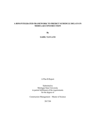
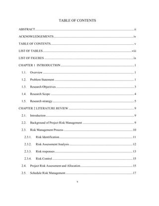
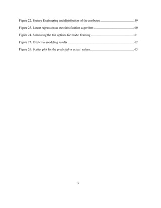
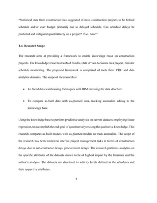
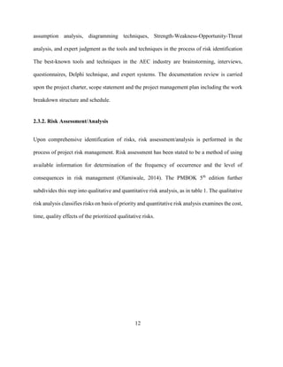
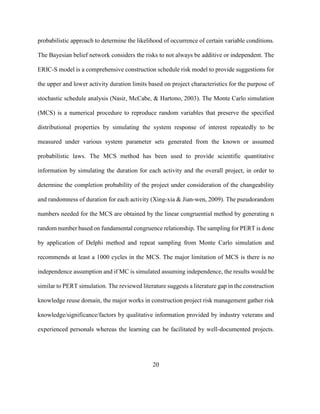
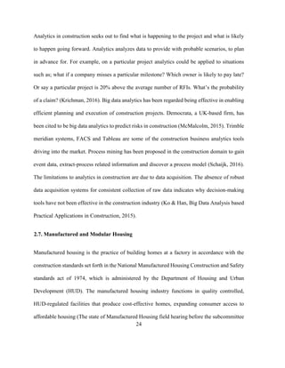
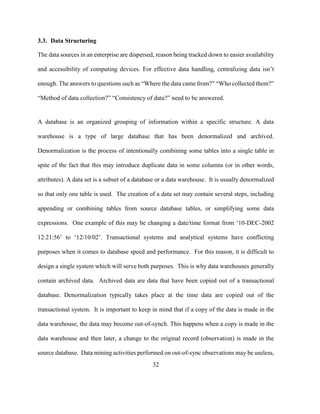
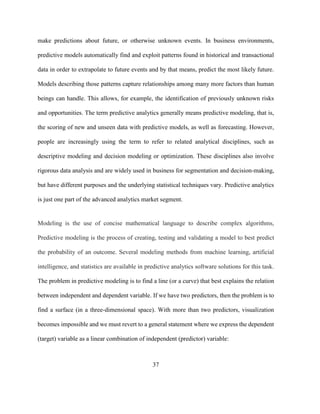
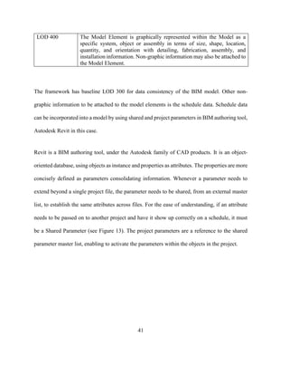
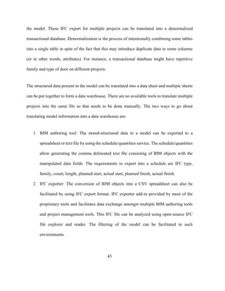
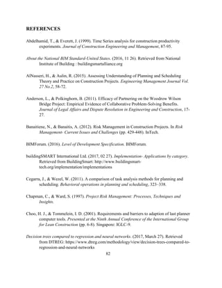
78
Cells.FormatConditions.Delete
End Sub
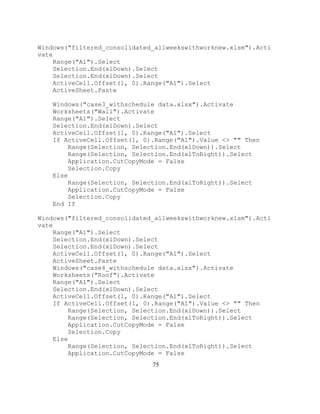
#3 Close the open sheets
Sub CloseBooks()
Application.DisplayAlerts = False
ActiveWorkbook.Close
End Sub
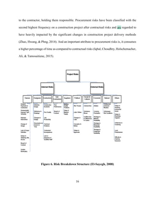
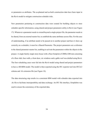
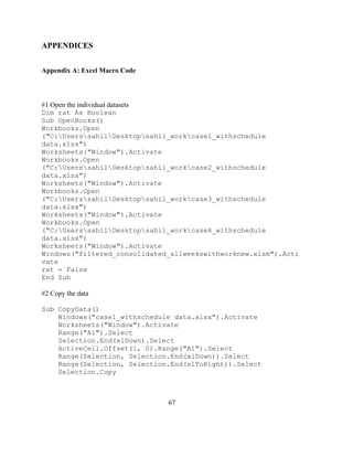
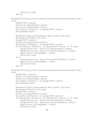
#4 Calculate duration and delay
Sub check_delay()
If Range("d6").Value = "" Then
MsgBox ("please copy the data")
Else
'To Claculate Which ever is greater days
Range("A1").Select
Selection.End(xlToRight).Select
Selection.End(xlUp).Select
ActiveCell.FormulaR1C1 = "=IF((RC[-6]-RC[-5])>(RC[-4]-RC[-
3]),(RC[-6]-RC[-5]),(RC[-4]-RC[-3]))"
Range("A1").Select
Range(Selection, Selection.End(xlUp)).Select
ActiveCell.FormulaR1C1 = ""
Selection.FormulaR1C1 = "=IF((RC[-6]-RC[-5])>(RC[-4]-RC[-
3]),(RC[-6]-RC[-5]),(RC[-4]-RC[-3]))"
'To Calculate Duration

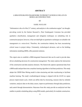
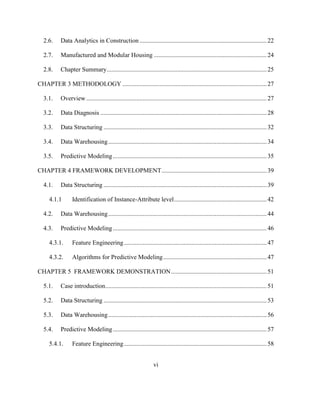
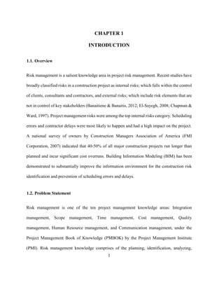
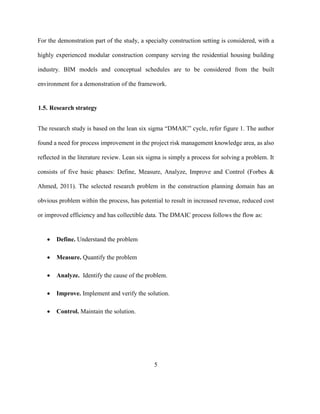
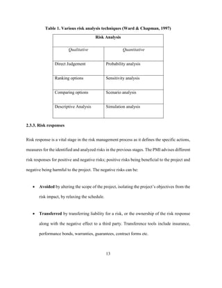
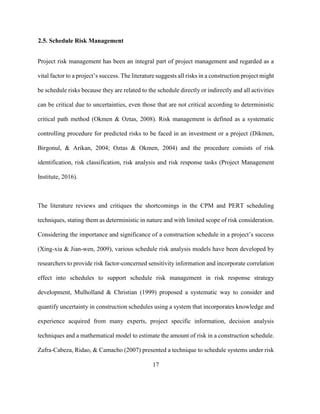
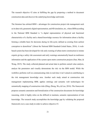
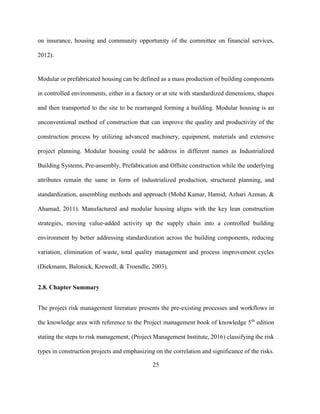
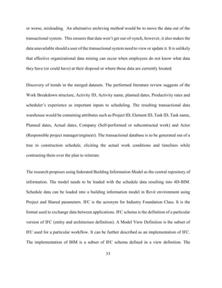
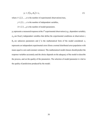
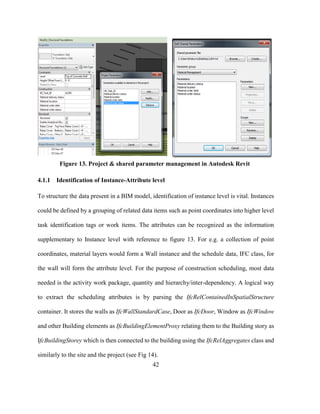
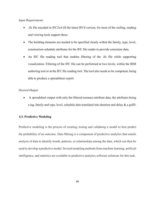
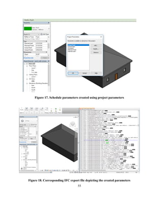
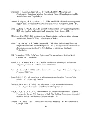
79
Range("A1").Select
Selection.End(xlUp).Select
ActiveCell.FormulaR1C1 = "(RC[-7]-RC[-5])"
Range("A1").Select
Range(Selection, Selection.End(xlUp)).Select
ActiveCell.FormulaR1C1 = ""
Selection.FormulaR1C1 = "=(RC[-7]-RC[-5])"
End If
End Sub

80
Appendix B: Weka Model Output
=== Run information ===
Scheme: weka.classifiers.functions.LinearRegression -S 0 -R 1.0E-8 -num-decimal-places
4
Relation: filtered_consolidated_allweeks-weka.filters.unsupervised.attribute.Remove-R1,3-
6,8
Instances: 52
Attributes: 4
Family and Type
Building Storey name
Duration
Delay
Test mode: split 66.0% train, remainder test
=== Classifier model (full training set) ===
Linear Regression Model
Delay =
1.4359 * Family and Type=M_Fixed: 0915 x 1830mm,M_Fixed: 0915 x
1220mm,M_Single-Flush: 0915 x 2134mm,Basic Wall: Generic - 200mm +
-0.6923
Time taken to build model: 0.05 seconds
=== Evaluation on test split ===
Time taken to test model on test split: 0 seconds
=== Summary ===
Correlation coefficient 0.1982
Mean absolute error 1.9444
Root mean squared error 2.4395
Relative absolute error 101.5358 %
Root relative squared error 97.2151 %

81
Total Number of Instances 18

82
REFERENCES
Abdelhamid, T., & Everett, J. (1999). Time Series analysis for construction productivity
experiments. Journal of Construction Engineering and Management, 87-95.
About the National BIM Standard-United States. (2016, 11 26). Retrieved from National
Institute of Building : buildingsmartalliance.org
AlNasseri, H., & Aulin, R. (2015). Assessing Understanding of Planning and Scheduling
Theory and Practice on Construction Projects. Engineering Management Journal Vol.
27 No.2, 58-72.
Anderson, L., & Polkinghorn, B. (2011). Efficacy of Partnering on the Woodrow Wilson
Bridge Project: Empirical Evidence of Collaborative Problem-Solving Benefits.
Journal of Legal Affairs and Dispute Resolution in Engineering and Construction, 17-
27.
Banaitiene, N., & Banaitis, A. (2012). Risk Management in Construction Projects. In Risk
Management- Current Issues and Challenges (pp. 429-448). InTech.
BIMForum. (2016). Level of Development Specification. BIMForum.
buildingSMART International Ltd. (2017, 02 27). Implementation- Applications by category.
Retrieved from BuildingSmart: http://www.buildingsmart-
tech.org/implementation/implementations
Cegarra, J., & Wezel, W. (2011). A comparison of task analysis methods for planning and
scheduling. Behavioral operations in planning and scheduling, 323–338.
Chapman, C., & Ward, S. (1997). Project Risk Management: Processes, Techniques and
Insights.
Choo, H. J., & Tommelein, I. D. (2001). Requirements and barriers to adaption of last planner
computer tools. Presented at the Ninth Annual Conference of the International Group
for Lean Construction (pp. 6-8). Singapore: IGLC-9.
Decision trees compared to regression and neural networks. (2017, March 27). Retrieved
from DTREG: https://www.dtreg.com/methodology/view/decision-trees-compared-to-
regression-and-neural-networks

83
Diekmann, J., Balonick, J., Krewedl, M., & Troendle, L. (2003). Measuring Lean
Conformance. Blacksburg, Virginia: International Group of Lean Construction 11th
Annual Conference Virginia Tech.
Dikmen, I., Birgonul, M. T., & Arikan, A. E. (2004). A Critical Review of Risk management
support tools. Association of researchers in construction management, 1145-1154.
Ding, L., Zhong, B., Wu, S., & Luo, H. (2016). Construction risk knowledge management in
BIM using ontology and semantic web technology. Safety Science, 202-213.
El-Sayegh, S. M. (2008). Risk assessment and allocation in the UAE construction industry.
International Journal of Project Management, 431-438.
Feng , C.-W., & Chen , Y.-J. (2008). Using the MD CAD model to develop the time-cost
integrated schedule for construction projects. The 25th symposium on Automation and
Robotics in construction (pp. 573-584). Institute of Internet and Intelligent
Technologies.
FMI Corporation. (2007). FMI/CMAA Eight Annual Survey of Owners. Raleigh, North
Carolina: FMI Corporation.
Forbes, L. H., & Ahmed, S. M. (2011). Modern construction: Lean project delivery and
integrated practices. Boca Raton, Florida: CRC Press.
Forbes, L., & Ahmed, S. (2010). Modern Construction: Lean Project Delivery and Integrated
Practices. CRC Press.
Genz, R. (2001). Why advocated need to rethink manufactured housing. Housing Policy
Debate, Vol 12 Issue 2, pp. 393-414.
Golfarelli, M., & Rizzi, S. (2010). Data Warehouse Design: Modern Principles and
Methodologies . New York: The McGraw-Hill Companies, Inc.
Han, S., Lee, T., & Ko, Y. (2014). Implementation of Construction Performance Database
Prototype for Curtain Wall Operation in High-Rise Building Construction. Journal of
Asian Architecture and Building Engineering, 149-156.
Haugan, G. T. (2002). Project Planning and Scheduling. Leesburg Pike, VA: Management
Concepts Press.

84
Herroelen, W., & Leus, R. (2001). On the merits and pitfalls of critical chain scheduling.
Journal of Operations Management, 19(5), 559-577.
Improving decision making in organizations. (2016, October 23). Retrieved from
www.cimaglobal.com
Inmon, W. H. (2005). Building the data warehouse, 4th Edition. Indianapolis, Indiana: Wiley
Publishing, Inc.
Iqbal, S., Choudhry, R. M., Holschemacher, K., Ali, A., & Tamosaitiene, J. (2015). Risk
management in construction projects. Technological and economic development of
economy, 65-78.
Kiviniemi, M., Sulankivi, K., Kahkonen, K., Makela, T., & Merivirta, M.-L. (2011). BIM-
based Safety Management and Communication for Building Construction. VTT
TIEDOTTEITA- Research Notes 2597. VTT Technical Research Center of Finland.
Ko, Y., & Han, S. (2015). Big Data Analysis based Practical Applications in Construction.
Int'l Conf. on Advances in Big Data Analytics, (pp. 121-122). Incheon, South Korea.
Ko, Y., & Han, S. (2015). Development of Construction Performance Monitoring
Methodology using the Bayesian Probabilistic Approach. Journal of Asian
Architecture and Building Engineering, 73-80.
Krichman, M. (2016, January 8). Business Intelligence vs. Business Analytics for
Construction Companies. Retrieved from Lantern Data Systems:
http://lanterndata.com/business-intelligence-vs-business-analytics-for-construction-
companies/
Kuang, Z. (2011). Risk Management in Construction Projects: Application of Risk
management in construction period. Bachelor of Architectural Technology and
Construction Management. Via University College, Horsens Campus, Denmark.
Learning data science: feature engineering. (2017, March 24). Retrieved from
www.simafore.com: http://www.simafore.com/blog/learning-data-science-feature-
engineering
Lee, E., Park, Y., & Shin, J. G. (2008). Large engineering project risk management using a
bayesian belief network. Expert systems with applications, 5880-5887.

85
Liu, Y., & Li, Y. (2014). Risk management of construction schedule by PERT with Monte
Carlo simulation. Applied Mechanics and Materials, 1646-1650.
Marr, B. (2016, April 19). How Big Data And Analytics Are Transforming The Construction
Industry. Retrieved from Forbes.com:
http://www.forbes.com/sites/bernardmarr/2016/04/19/how-big-data-and-analytics-are-
transforming-the-construction-industry/#655e7f7c5cd0
McMalcolm, J. (2015, January 27). How big data is transforming the construction industry.
Retrieved from Construction Global:
http://www.constructionglobal.com/equipmentit/399/How-big-data-is-transforming-
the-construction-industry
Mohd Kamar, K. A., Hamid, Z. A., Azhari Azman, M. N., & Ahamad, M. S. (2011).
Industrialized Building System (IBS): revisiting issues of definition and classification.
International Journal of Emerging Sciences, 120-132.
Mongalo, M., & Lee, J. (1990). A Comparative-Study of methods for probabilistic project
scheduling. Computers & Industrial Engineering vol. 19, 505-509.
Mulholland, B., & Christian, J. (1999). Risk assessment in construction schedules. Journal of
Construction Engineering and Management, 8-15.
Nasir, D., McCabe, B., & Hartono, L. (2003). Evaluating RIsk in Construction- Schedule
Model (ERIC-S): Construction Risk schedule model. Journal of Construction
Engineering and Management, 518-527.
North, M. (2012). Data Mining for the Masses.
Nyce, C. (2007). Predictive analytics white paper. Malvern, PA: American Institute for
Chartered Property Casual Underwriters/Insurance Institute of America.
Okmen, O., & Oztas, A. (2008). Construction Project Network Evaluation with correlated
schedule risk analysis model. Journal of Construction Engineering and Management,
49-63.
Olamiwale, I. (2014). Evaluation of Risk Management Practices in the Construction Industry
in Swaziland. Master of Quantity Surveying Thesis, Tshwane University of
Technology, Pretoria, South Africa.

86
Oztas, A., & Okmen, O. (2004). Risk analysis in fixed-price design–build construction
projects. Building and Environment, 229-237.
Project Management Institute. (2016). Project Management Book of Knowledge.
Renault, B. Y., & Agumba, J. N. (2016). Risk management in the construction industry: a
new literature review. MATEC Web of Conferences, 1-6.
Renault, B. Y., Agumba, J. N., & Balogun, O. A. (2016 26-28 June). Drivers for and
Obstacles to Enterprise Risk Management in COnstruction Firms: A literature
Review. Creative Construction Conference 2016, (pp. 167-172). Budapest, Hungary.
Ribeiro, F. L. (2009). "Enhancing knowledge management in construction firms.
Construction Innovation, Vol. 9 Iss 3, 268-284.
Saidi, K. S., Lytle, A. M., & Stone, W. C. (2003). Report of the NIST workshop on data
exchange standards at the construction job site.
Schaijk, S. V. (2016). Building Information Model (BIM) based process mining. Eindhoven,
Netherland: Eindhoven University of Technology.
Shevchenko, G., Ustinovichius, L., & Andruskevicius, A. (2008). Multi-attribute analysis of
investments risk alternatives in construction. Technological and economic
development of economy, 14(3), 428-443.
Simu, K. (2006). Risk management in small construction projects. Licentiate dissertation,
Department of Civil and Environmental Engineering. Lulca: LTU.
Smith, D. K., & Tardif, M. (2009). Building Information Modeling: A stratergic
Implementation Guide for Architects, Engineers, Constructors, and Real Estate
Managers. Hoboken, NJ: John Wiley & Sons, Inc.
Sun, C., Man, Q., & Wang, Y. (2015). Study on BIM-based construction project cost and
schedule risk early warning. Journal of Intelligent & Fuzzy Systems, 469-477.
(2012). The state of Manufactured Housing field hearing before the subcommittee on
insurance, housing and community opportunity of the committee on financial services.
Washington: U.S. House of Representatives, 112th Congress, First Session,
November 29, 2011.

87
Weka 3: Data Mining Software in Java. (2017, 03 31). Retrieved from Machine Learning
Group at the University of Waikato: http://www.cs.waikato.ac.nz/ml/weka/
Wirth, R., & Hipp, J. (2000). CRISP-DM: Towards a Standard Process Model for Data.
Proceedings of the 4th international conference on the practical applications of
knowledge discovery and data mining, (pp. 29-39).
Xing-xia, W., & Jian-wen, H. (2009). Risk Analysis of construction schedule based on monte
carlo simulation. 2009 International Conference on Information Management,
Innovation Management and Industrial Engineering, (pp. 150-153).
Yang, J. B. (2005). Comparison of CPM and CCS tools to construction project. Proceedings
of Third International Structural Engineering and Construction Conference (pp. 845-
851). Shunan, Japan: ISEC 03.
Yim, N. H., Kim, S. H., Kim, H. W., & Kwahkc, K. Y. (2004). Knowledge based decision
making on higher level strategic concerns: system dynamics approach. Expert Systems
with Applications, Vol. 27 No. 1, 143-158.
Zafra-Cabeza, A., Ridao, M. A., & Camacho, E. F. (2007). A model predictive control
approach for project risk management. European Control Conference 2007, (pp.
3337-3343). Kros, Greece.
Zaïane, O. R. (1999). Chapter I: Introduction to Data Mining . CMPUT690 Principles of
Knowledge Discovery in Databases . Alberta, Canada: Dpartment of Computing
Science, University of Alberta.
Zavadskas, E. K., Turskis, Z., & Tamosaitiene, J. (2010). Risk assessment of construction
projects. Journal of Civil Engineering and Management 16(1), 33-46.
Zhao, X., Hwang, B.-G., & Phng, W. (2014). Construction project risk management in
Singapore: Resources, effectiveness, impact, and understanding. KSCE Jornal of Civil
Engineering, 27-36.

BIM-Integrated predictive model for schedule delays in Construction

More Related Content

Similar to BIM-Integrated predictive model for schedule delays in Construction

Recently uploaded

BIM-Integrated predictive model for schedule delays in Construction