I am a BBA (Hons) student

1. Financial Management refers to the planning, organizing, directing, and controlling of financial
resources in an organization or individual’s life to achieve their financial goals. It involves
decisions related to investments, financing, dividends, and managing resources efficiently. A
strong financial management system helps organizations and individuals use their financial
resources wisely, ensuring that they meet short-term and long-term goals.
Here's a deeper look at key areas within financial management, along with some practical
examples:
1. Investment Decisions (Capital Budgeting)
 Definition: Investment decisions involve determining which projects or assets a company
should invest in, in order to maximize returns. It includes evaluating potential
investments, deciding which ones to pursue, and allocating funds accordingly.
 Key Concepts:
o Net Present Value (NPV): The difference between the present value of cash
inflows and outflows over a period of time. A positive NPV indicates a good
investment.
o Internal Rate of Return (IRR): The discount rate at which the NPV of all cash
flows from a project equals zero. It helps in evaluating the profitability of an
investment.
 Example: Imagine a company that wants to decide between two projects:
o Project A has an expected return of $500,000, and its NPV is $100,000.
o Project B has an expected return of $450,000, and its NPV is $120,000. The
company would likely invest in Project B, as it provides a higher return relative
to its cost.
2. Financing Decisions (Capital Structure)
 Definition: Financing decisions concern how a company raises capital to fund its
operations and investments. These decisions revolve around the mix of debt and equity
used by a company to finance its activities.
 Key Concepts:
o Debt Financing: Borrowing money, usually in the form of loans or bonds.
o Equity Financing: Raising capital by issuing shares of stock.
o Optimal Capital Structure: The balance between debt and equity that minimizes
the cost of capital and maximizes shareholder value.
 Example: A company might face a choice between issuing new stock or borrowing
money through bonds to raise $1 million for an expansion project.
o Debt Option: Issue bonds with an interest rate of 5%, but the company will have
to repay principal and interest.
o Equity Option: Issue 100,000 new shares at $10 per share. While there is no
repayment obligation, the company will dilute the ownership of current
shareholders. The company’s financial manager would need to calculate which
option minimizes costs and risk while maximizing shareholder value.

2. 3. Dividend Decisions
 Definition: Dividend decisions are concerned with how much of a company's earnings
should be distributed to shareholders as dividends and how much should be retained for
reinvestment.
 Key Concepts:
o Dividend Payout Ratio: The proportion of earnings paid out as dividends.
o Retention Ratio: The proportion of earnings retained in the business.
o Stable Dividends: Companies may aim for a stable or gradually increasing
dividend to maintain investor confidence.
 Example: A company earns $10 million in profit and decides that 40% will be paid as
dividends ($4 million), while 60% ($6 million) will be retained to fund growth initiatives
such as expansion or R&D.
4. Working Capital Management
 Definition: Working capital management involves managing short-term assets and
liabilities to ensure that a company has enough liquidity to meet its day-to-day
operational needs.
 Key Concepts:
o Current Assets: Cash, accounts receivable, and inventory.
o Current Liabilities: Short-term debts, accounts payable, and accrued expenses.
o Cash Conversion Cycle: The time it takes for a company to convert its
investments in inventory and accounts receivable into cash.
 Example: A retail company needs to ensure that it has enough inventory on hand to meet
demand, while also managing accounts payable and receivable efficiently. If the
company has $2 million in accounts receivable and $1.5 million in accounts payable,
managing the timing of collections and payments is critical to maintaining liquidity.
5. Risk Management
 Definition: Risk management in financial management involves identifying, analyzing,
and mitigating the financial risks that a company may face. These risks may include
market risk, credit risk, operational risk, and others.
 Key Concepts:
o Hedging: Using financial instruments like options or futures to offset potential
losses.
o Diversification: Spreading investments across different assets or markets to
reduce risk.
 Example: A company in the oil industry might use futures contracts to lock in oil prices
to protect itself from future price fluctuations. Alternatively, it might diversify its
investment portfolio to include stocks, bonds, and international assets to reduce exposure
to a single market.
6. Financial Reporting and Analysis

3.  Definition: Financial reporting involves preparing and analyzing financial statements,
which provide insights into a company's financial performance. Key reports include the
Income Statement, Balance Sheet, and Cash Flow Statement.
 Key Concepts:
o Profitability Ratios: Measures like Return on Equity (ROE), Return on Assets
(ROA), and profit margin.
o Liquidity Ratios: Measures like the current ratio and quick ratio to determine if
the company can meet its short-term obligations.
o Leverage Ratios: Measures of a company’s debt levels, such as the debt-to-
equity ratio.
 Example: A company may analyze its Return on Assets (ROA) to determine how
efficiently it is using its assets to generate profit. If the ROA is 5%, it means the company
is generating $0.05 in profit for every dollar of assets.
Summary
In financial management, these areas (investment decisions, financing decisions, dividend
decisions, working capital management, risk management, and financial reporting) all work
together to ensure that resources are effectively utilized to achieve the financial goals of an
organization or individual. By making informed decisions, companies can maximize their value,
reduce risk, and maintain a healthy financial position.
If you’d like to go deeper into any of these topics, feel free to ask!
Business Finance and Management is a broad and complex field that involves managing a
company’s financial resources, making investment and funding decisions, and ensuring the
efficient operation of financial activities to achieve organizational goals. It's concerned with
obtaining, allocating, and using financial resources to ensure that the business can meet its
objectives and grow.
Here, we’ll explore business finance and management in depth, covering the major aspects and
providing real-world examples:
1. Financial Management

4. Financial management is about overseeing and managing a company’s financial activities,
including investments, budgeting, and cash flow management. It aims to maximize shareholder
wealth and ensure the company has enough capital to function effectively.
Key Elements:
 Investment Decisions (Capital Budgeting): Deciding where and how to allocate financial
resources for the company's long-term growth.
 Financing Decisions (Capital Structure): Determining how to finance investments,
whether through debt, equity, or internal cash flows.
 Dividend Decisions: Deciding how much profit should be distributed to shareholders
versus retained for reinvestment.
Example:
A company like Tesla may need to decide whether to use its retained earnings or issue new
equity to fund its next major research project. If it issues equity, it risks diluting current
shareholders, but if it uses debt financing, it incurs interest expenses.
2. Capital Budgeting and Investment Decisions
Capital budgeting refers to the process of evaluating and selecting long-term investment
opportunities that are expected to generate returns over time. This is essential for the company’s
growth and sustainability.
Methods Used:
 Net Present Value (NPV): Calculates the difference between the present value of cash
inflows and outflows. A project with a positive NPV is typically considered a good
investment.
 Internal Rate of Return (IRR): The discount rate that makes the NPV of a project zero.
If the IRR exceeds the company's required return, the project is acceptable.
 Payback Period: Measures how long it takes for an investment to recover its initial cost.
 Profitability Index: A ratio that compares the present value of future cash inflows to the
initial investment.
Example:
A company is evaluating two projects:
 Project A: Requires an initial investment of $1 million and is expected to generate
$300,000 per year for 5 years. The NPV is $500,000.
 Project B: Requires an initial investment of $1.5 million and generates $400,000
annually for 5 years. The NPV is $450,000.
Based on NPV, the company would choose Project A because it provides a higher return
for a lower initial investment.

5. 3. Working Capital Management
Working capital management involves managing the short-term assets and liabilities of the
business to ensure it has enough liquidity to meet its operational needs.
Components of Working Capital:
 Current Assets: Cash, accounts receivable, inventory.
 Current Liabilities: Accounts payable, short-term debt.
Key Ratios:
 Current Ratio = Current Assets ÷ Current Liabilities. This ratio indicates if the business
can pay its short-term debts.
 Quick Ratio = (Current Assets - Inventory) ÷ Current Liabilities. This is a more stringent
test of liquidity.
 Cash Conversion Cycle: Measures how long it takes for a company to convert its
investments in inventory and receivables into cash.
Example:
A retail business may keep a large inventory of products. If the inventory turnover ratio is low, it
could indicate that products are sitting unsold for a long time, tying up cash. Effective working
capital management would involve reducing excess inventory or improving the collection of
receivables to improve cash flow.
4. Financing Decisions (Capital Structure)
Financing decisions involve determining the optimal mix of debt (loans, bonds) and equity
(stocks, retained earnings) for the company. The goal is to minimize the cost of capital and
maximize shareholder wealth.
Key Concepts:
 Debt Financing: Borrowing funds that need to be repaid, often with interest. It can be in
the form of loans, bonds, or other debt instruments.
 Equity Financing: Raising capital by issuing shares to investors, diluting ownership but
not incurring debt.
 Optimal Capital Structure: The mix of debt and equity that minimizes the cost of
capital and maximizes the value of the firm.
Example:
Apple Inc. is a good example of how capital structure can evolve over time. Apple once relied

6. heavily on debt to finance its operations, but as the company grew and became more profitable, it
shifted toward using more equity financing. This allowed them to preserve financial flexibility
while still returning value to shareholders.
5. Financial Reporting and Analysis
Business finance involves preparing accurate financial reports and analyzing the company's
financial health. The three primary financial statements are:
 Income Statement: Shows the company’s revenues, costs, and profits over a period.
 Balance Sheet: Provides a snapshot of the company’s assets, liabilities, and equity at a
point in time.
 Cash Flow Statement: Shows the inflow and outflow of cash, indicating the company's
liquidity and ability to meet its short-term obligations.
Key Ratios for Analysis:
 Profitability Ratios (e.g., ROE, ROA, Gross Margin).
 Liquidity Ratios (e.g., Current Ratio, Quick Ratio).
 Solvency Ratios (e.g., Debt-to-Equity Ratio, Interest Coverage Ratio).
Example:
Consider Amazon. By analyzing its financial statements, Amazon’s management can assess its
profitability (through metrics like gross margin) and liquidity (through the current ratio). In
2020, despite massive growth, Amazon focused on improving cash flow and minimizing debt,
ensuring it had enough liquidity to handle disruptions like the COVID-19 pandemic.
6. Risk Management
Managing financial risks involves identifying potential risks, assessing their impact, and
developing strategies to minimize or avoid them. These risks can include market risk, credit risk,
liquidity risk, operational risk, etc.
Techniques for Managing Financial Risk:
 Hedging: Using financial instruments like futures, options, or swaps to mitigate potential
losses from changes in market conditions.
 Diversification: Spreading investments across different assets or markets to reduce
exposure to any one risk.
 Insurance: Purchasing policies to protect the business against potential losses, such as
property damage, liability claims, or cyber risks.

7. Example:
Airlines often face fuel price fluctuations, so they might use fuel hedging to lock in fuel prices
for a period to reduce the uncertainty of operating costs. A company like Southwest Airlines is
well known for using hedging strategies to stabilize its fuel costs, especially when oil prices are
volatile.
7. Strategic Financial Management
Strategic financial management focuses on aligning the company’s financial management with
its broader strategic goals. This can involve mergers and acquisitions (M&A), expansion
strategies, and other large-scale initiatives.
Example:
Google’s acquisition of YouTube in 2006 for $1.65 billion is a prime example of a strategic
financial decision. Google recognized the growing power of video content and wanted to ensure
it had a platform to compete with emerging competitors. From a financial perspective, this
acquisition was a long-term investment that paid off by greatly expanding Google’s market share
in digital advertising.
Conclusion
Business Finance and Management plays a pivotal role in ensuring that a company’s financial
resources are used effectively to generate profit, minimize risk, and drive growth. By making
informed decisions about investments, financing, risk management, and reporting, businesses can
remain competitive and achieve long-term success.
Real-world companies like Tesla, Apple, Amazon, and Google offer practical examples of how
financial management practices are applied to drive growth, manage risk, and deliver value to
shareholders. Effective financial management provides businesses with the tools and insights
they need to make sound financial decisions that align with their strategic objectives.
Let me know if you'd like to dive deeper into any of these areas!
Forms of Business Organization refer to the legal structures under which a business can
operate. Each structure has its own set of rules, advantages, and disadvantages, and the choice of

8. business form depends on various factors, such as the type of business, the level of liability, the
desired tax treatment, and the goals of the owners.
Let’s explore the main forms of business organization in-depth, along with examples:
1. Sole Proprietorship
 Definition: A sole proprietorship is the simplest and most common form of business
organization. It is owned and operated by a single individual who has complete control
over all aspects of the business. The owner is responsible for all profits, losses, and
liabilities.
 Key Features:
o Ownership: One individual owns and controls the business.
o Liability: The owner has unlimited personal liability for all business debts and
obligations.
o Taxation: Profits are taxed as personal income, avoiding double taxation.
o Management: The owner makes all decisions.
o Continuity: The business ends if the owner dies or decides to close it.
 Advantages:
o Easy to set up and dissolve.
o Full control over decision-making.
o No corporate taxation; all income is reported on the owner’s personal tax return.
 Disadvantages:
o Unlimited personal liability for business debts.
o Limited ability to raise capital or expand.
o May be harder to attract high-level talent or investors.
 Example:
A local freelance graphic designer or plumber running a one-person business would
typically operate as a sole proprietorship. The owner handles all clients, finances, and
business decisions independently, without sharing profits or losses with anyone else.
2. Partnership
 Definition: A partnership is a business structure where two or more individuals (or
entities) share ownership and the responsibilities of running a business. There are two
main types of partnerships: general partnerships and limited partnerships.
 Key Features:
o Ownership: Two or more partners share ownership of the business.
o Liability: In a general partnership, all partners share equal responsibility for the
business's debts. In a limited partnership, one or more partners have limited
liability, while others have unlimited liability.
o Taxation: Profits and losses are passed through to the partners and taxed on their
personal returns (avoiding corporate taxation).

9. o Management: Management is shared among the partners, unless otherwise
specified in the partnership agreement.
o Continuity: The partnership may dissolve if one partner dies or withdraws, unless
a continuity agreement is in place.
 Advantages:
o Easier to raise capital compared to a sole proprietorship.
o Shared responsibilities and resources among partners.
o Tax benefits due to pass-through taxation.
 Disadvantages:
o Unlimited liability for general partners.
o Potential for conflict between partners.
o Partners may be personally liable for the actions of others.
 Example:
Ben & Jerry's was originally a partnership between Ben Cohen and Jerry Greenfield,
who started a small ice cream shop together. They shared the profits, responsibilities, and
risks involved in the business, until they sold to Unilever.
3. Limited Liability Company (LLC)
 Definition: A Limited Liability Company (LLC) is a hybrid business structure that
combines the limited liability features of a corporation with the tax efficiencies and
operational flexibility of a partnership.
 Key Features:
o Ownership: Owners of an LLC are called members.
o Liability: Members have limited liability, meaning their personal assets are
protected from business debts and legal actions.
o Taxation: LLCs typically benefit from pass-through taxation where profits and
losses are reported on members' personal tax returns. However, LLCs can choose
to be taxed as a corporation.
o Management: An LLC can be managed by its members (member-managed) or
by designated managers (manager-managed).
o Continuity: An LLC can continue to exist even if a member leaves or dies.
 Advantages:
o Limited liability protection for owners.
o Flexible management structure.
o Pass-through taxation.
o Fewer formalities compared to a corporation.
 Disadvantages:
o Can be more expensive and complex to form than a sole proprietorship or
partnership.
o Some states impose additional taxes or fees on LLCs.
 Example:
A small business like a local tech startup or consulting firm might choose to form an
LLC to take advantage of limited liability protection and pass-through taxation. For

10. instance, Etsy, an e-commerce platform, initially operated as an LLC before expanding
into a corporation.
4. Corporation (C-Corp and S-Corp)
 Definition: A corporation is a legal entity that is separate and distinct from its owners,
providing limited liability to shareholders. The corporation can enter into contracts, own
property, sue, and be sued in its own name.
 Key Features:
o Ownership: Owned by shareholders who hold stock in the company.
o Liability: Shareholders have limited liability; they are not personally responsible
for the corporation's debts or legal issues.
o Taxation:
 C-Corp: The corporation is taxed separately from its owners. The
corporation’s profits are taxed at the corporate rate, and dividends paid to
shareholders are taxed again on the individual level (double taxation).
 S-Corp: An S-Corp is a special tax status that allows income, deductions,
and credits to be passed through to shareholders for federal tax purposes,
avoiding double taxation.
o Management: Managed by a board of directors who make major decisions, and
executives (e.g., CEO) who handle daily operations.
o Continuity: A corporation exists independently of the owners and can continue
indefinitely.
 Advantages:
o Limited liability protection for shareholders.
o Ability to raise capital by issuing stock.
o Continuity of existence regardless of changes in ownership.
 Disadvantages:
o Double taxation for C-Corporations.
o Expensive and time-consuming to set up and maintain (with more regulations).
o More complex management and governance structure.
 Example:
Apple Inc. is a prominent example of a corporation. As a publicly traded company,
Apple has millions of shareholders, and its stock is traded on the stock market. The
company is managed by a board of directors and a team of executives.
5. Cooperative (Co-op)
 Definition: A cooperative is a business owned and operated by a group of individuals for
their mutual benefit. Co-ops are typically formed to meet the common needs of their
members, such as reducing costs, sharing resources, or accessing services.
 Key Features:

11. o Ownership: Co-ops are owned and controlled by their members, who may be
customers, workers, or producers.
o Liability: Members have limited liability, similar to an LLC.
o Taxation: Co-ops enjoy tax advantages, especially in agricultural or consumer
co-ops, since profits are typically returned to the members.
o Management: Managed democratically, with each member having a vote in
decision-making, regardless of their contribution.
o Continuity: Like corporations, co-ops can continue even if members leave or die.
 Advantages:
o Collective ownership and control.
o Often have tax benefits.
o Focused on member benefits rather than maximizing profits.
 Disadvantages:
o Decision-making can be slow and cumbersome due to democratic structure.
o May face challenges in raising capital.
 Example:
Ocean Spray is an agricultural cooperative owned by cranberry farmers. The cooperative
allows farmers to pool their resources, improve production efficiency, and share in the
profits generated from selling cranberry products.
Conclusion
Each form of business organization offers distinct advantages and challenges based on the
nature of the business, the desired level of liability protection, and the tax implications. Here’s a
quick summary:
 Sole Proprietorship: Best for small businesses where the owner wants full control and
responsibility.
 Partnership: Suitable for two or more individuals who want to share control, profits, and
risks.
 LLC: Offers flexibility with limited liability, ideal for small to medium-sized businesses.
 Corporation: Best for businesses looking to raise capital through stock issuance and
protect owners from liability.
 Cooperative: Great for organizations formed to meet the collective needs of members,
often in industries like agriculture or retail.
Each business form has its own set of rules that dictate how it operates, and the choice of
structure should align with the business’s goals, size, and future plans. Let me know if you'd like
more details on any specific form or examples!
The goals of business finance are central to how a company operates, grows, and maximizes
value. These goals guide decisions about investments, capital structure, and resource allocation

12. to achieve long-term financial stability and success. Understanding the key financial goals can
help a business align its strategies and ensure it remains financially healthy while achieving its
broader objectives.
Let’s explore the key goals of business finance in-depth, along with examples:
1. Maximizing Shareholder Wealth
 Definition: The primary goal of business finance for most companies, especially publicly
traded ones, is to maximize the wealth of shareholders. This typically involves increasing
the value of the company’s stock and providing returns through dividends and capital
appreciation.
 Key Concepts:
o Stock Price Appreciation: A company’s success and profitability are reflected in
its stock price. When the company performs well, the stock price typically rises,
benefiting shareholders.
o Dividends: Many companies pay dividends to shareholders as a portion of their
profits, which contributes to the overall wealth of the shareholders.
 Why It’s Important: Maximizing shareholder wealth aligns with the goal of creating
value for investors, who provide capital to the company. It also attracts more investors,
which can lead to increased capital and opportunities for growth.
 Example:
Apple Inc. is a prime example of maximizing shareholder wealth. Over the years, Apple
has focused on increasing its stock price and regularly returning profits to shareholders
through dividends and share buybacks. As a result, the company's stock has experienced
significant appreciation, creating immense value for its shareholders.
2. Profit Maximization
 Definition: Profit maximization is the goal of generating the highest possible profit for
the business, which directly impacts the financial success of the company. It focuses on
the balance between revenue and costs.
 Key Concepts:
o Revenue Generation: Increasing sales or creating new revenue streams.
o Cost Control: Reducing operating costs, overhead, and inefficiencies to
maximize profit.
 Why It’s Important: Profit maximization is fundamental for any business because it
provides the financial resources needed to reinvest in the company, pay shareholders, and
sustain growth. However, it’s important to note that this goal should be balanced with
other factors like risk and sustainability.
 Example:
Amazon has focused on profit maximization by scaling its e-commerce operations

13. globally. The company focuses on increasing its revenue through product sales while also
managing its costs, such as optimizing supply chain operations and using technology to
reduce labor expenses. Amazon’s profitability has allowed it to reinvest in new ventures,
expanding into cloud computing (AWS), which has become a massive source of revenue.
3. Ensuring Liquidity (Solvency)
 Definition: Liquidity refers to the ability of a business to meet its short-term financial
obligations as they come due. Solvency refers to the long-term financial stability of a
business—its ability to meet all financial obligations, both short-term and long-term.
 Key Concepts:
o Current Ratio: A liquidity ratio that measures the ability of a business to cover
its short-term liabilities with its short-term assets. A ratio of 2:1 is often
considered healthy.
o Quick Ratio: A more stringent measure of liquidity, excluding inventory from
current assets. It helps assess a company’s ability to meet short-term obligations
without selling inventory.
o Cash Flow Management: Ensuring the company has sufficient cash flow to meet
obligations, pay employees, suppliers, and maintain operations.
 Why It’s Important: Without adequate liquidity, a company could struggle to pay its
bills, employees, or creditors, leading to operational disruptions or even bankruptcy.
Solvency is also crucial for maintaining investor confidence and creditworthiness.
 Example:
Tesla in its earlier years faced liquidity challenges as it needed significant capital to fund
its operations and expansion. The company had to secure financing from investors to stay
afloat. Over time, by focusing on growing its revenues, Tesla improved its cash flow and
liquidity, helping it to become solvent and continue its mission of scaling production.
4. Risk Management
 Definition: Risk management in business finance involves identifying, analyzing, and
managing the financial risks a company faces. Risks can include market risk, operational
risk, credit risk, or external factors like economic downturns or regulatory changes.
 Key Concepts:
o Hedging: Financial instruments like options and futures can be used to offset or
minimize risks, particularly in areas like commodity prices, interest rates, and
foreign exchange rates.
o Diversification: Spreading investments across various assets, industries, or
geographic areas to reduce the impact of risk.
o Insurance: Purchasing insurance policies to protect against specific risks, such as
property damage or liability claims.

14.  Why It’s Important: Effective risk management helps protect the business from
unforeseen events and reduces the likelihood of financial distress. Companies that
manage risk well are often more resilient in the face of challenges and better able to
thrive in volatile markets.
 Example:
Southwest Airlines is known for its hedging strategy to manage the risk of volatile fuel
prices. By locking in fuel prices ahead of time using financial instruments, Southwest
minimized the impact of sudden increases in fuel costs, allowing it to maintain
profitability even during times of rising oil prices.
5. Capital Structure Optimization
 Definition: Capital structure refers to the mix of debt and equity financing a company
uses to fund its operations and growth. The goal is to find the optimal balance that
minimizes the cost of capital while maintaining enough flexibility and liquidity.
 Key Concepts:
o Debt Financing: Borrowing money through loans or issuing bonds. Debt often
comes with fixed interest costs, but it can be tax-deductible and leverage a
company's growth.
o Equity Financing: Raising capital by issuing shares of stock. Equity financing
doesn’t require repayment, but it dilutes ownership and may limit control.
o Cost of Capital: The overall cost of financing, including the cost of debt and
equity. The goal is to minimize this cost to maximize value.
 Why It’s Important: An optimal capital structure helps the company maximize its value
by reducing financing costs and minimizing risks. The structure impacts everything from
financial stability to the company’s ability to invest in future growth opportunities.
 Example:
Microsoft has historically maintained a strong balance between debt and equity, using a
mix of retained earnings, equity issuance, and some debt financing. This allowed
Microsoft to invest heavily in product development and acquisitions, while maintaining a
relatively low debt load to avoid excessive financial risk.
6. Sustainability and Corporate Social Responsibility (CSR)
 Definition: Increasingly, businesses are aligning their financial goals with sustainability
and corporate social responsibility. This involves making decisions that support
environmental and social goals while maintaining profitability.
 Key Concepts:
o Environmental Sustainability: Ensuring that business practices do not harm the
environment and that resources are used efficiently.
o Social Responsibility: Acting in ways that benefit society, including fair labor
practices, philanthropy, and community development.

15. o Triple Bottom Line (TBL): A framework that evaluates a company’s social,
environmental, and financial performance.
 Why It’s Important: Companies that embrace sustainability and CSR tend to have a
positive brand image, attract socially-conscious consumers, and maintain long-term
viability by adapting to societal and environmental challenges.
 Example:
Patagonia is an excellent example of a company that integrates sustainability with its
financial goals. The company invests in eco-friendly production practices, promotes fair
labor practices, and donates a portion of its profits to environmental causes. Patagonia’s
commitment to sustainability has bolstered its brand and attracted a loyal customer base.
Conclusion
In business finance, the primary goals are interlinked but distinct. The most important goals
include:
1. Maximizing Shareholder Wealth – Achieving higher stock prices and providing returns
to shareholders.
2. Profit Maximization – Ensuring the business is generating the highest possible profit.
3. Ensuring Liquidity and Solvency – Ensuring the company can meet short-term and
long-term obligations.
4. Risk Management – Identifying and mitigating potential financial risks.
5. Capital Structure Optimization – Balancing debt and equity financing to minimize cost
and risk.
6. Sustainability and CSR – Integrating social and environmental goals with financial
objectives.
Each of these goals plays a vital role in the financial health and long-term success of the
company. By balancing profitability, risk, and long-term value creation, businesses can achieve
their financial objectives and thrive in a competitive environment.
If you'd like more details on any of these goals, or specific examples, feel free to ask!
Agency Problem: In-Depth Explanation
The agency problem arises from the conflicts of interest that can occur when one party (the principal)
delegates decision-making authority to another party (the agent). In the context of business, this

16. situation typically involves shareholders (principals) hiring managers (agents) to run the company on
their behalf. While the principal and agent ideally have aligned interests, differences in their objectives,
risk preferences, and incentives can create agency conflicts.
Key Concepts:
 Principal: The person or entity that owns the resources or assets and delegates authority. In a
corporation, shareholders are the principals, as they own the company.
 Agent: The individual or group hired by the principal to manage or operate the business. In a
corporation, the managers or executives are the agents.
 Agency Cost: The costs that arise from resolving conflicts between principals and agents. These
costs can include monitoring costs, bonding costs, and the residual loss from not perfectly
aligning the interests of the two parties.
Why Does the Agency Problem Occur?
1. Divergent Objectives:
o Shareholders (Principals): Typically, the goal of shareholders is to maximize the value of
the company over the long term, reflected in the stock price and overall profitability.
Their interests are tied to the performance of the company.
o Managers (Agents): Managers may have goals that differ from shareholders’ interests,
such as increasing their own compensation, securing job stability, or pursuing personal
career goals, even at the cost of the company’s long-term performance.
2. Information Asymmetry:
o Asymmetry of Information: Managers often have more information about the day-to-
day operations of the business than shareholders. This gives managers the ability to
make decisions without fully revealing the information to the principals.
o Hidden Actions and Hidden Information: Managers might act in ways that are beneficial
to them (e.g., pursuing projects with short-term gains) rather than focusing on
maximizing shareholder wealth in the long run.
3. Moral Hazard:
o The agent may take actions that benefit themselves but harm the principal. For
instance, managers may take excessive risks with the company’s resources because they
don’t bear the full consequences of failure (since they don’t typically lose personal
wealth if the business fails).
4. Lack of Effective Monitoring:
o Shareholders cannot always monitor every decision made by managers due to costs and
practical limitations. Therefore, agents might exploit this by acting in ways that are not
in the best interest of the principal.
Types of Agency Problems

17. 1. Ownership vs. Control:
o In large corporations, the owners (shareholders) do not usually manage the business
themselves. Instead, they hire professional managers to do so. This creates a conflict
because managers may act in their own interest rather than the shareholders' best
interest.
o Example: A publicly traded company has many shareholders (owners) but a
management team running the company. The management might engage in actions
that improve their position (e.g., increasing personal perks, such as luxury office spaces
or higher salaries), even if these actions don’t align with the goal of maximizing
shareholder wealth.
2. Shareholders vs. Debt Holders:
o Shareholders typically prefer high-risk, high-reward strategies, as they benefit from
higher returns. Debt holders (creditors), however, prefer more conservative strategies
because they want to ensure their loans are repaid without risk.
o Example: A company that is highly leveraged (with significant debt) might make riskier
investments, which could benefit shareholders if the investments succeed, but
jeopardize the debt holders' capital if they fail.
Examples of the Agency Problem in Practice
Example 1: CEO Compensation and Performance
One of the classic examples of an agency problem is executive compensation. Managers might push for
higher salaries, stock options, or bonuses that are not directly tied to long-term performance. They
might receive lucrative compensation packages that provide immediate rewards even if their actions
don’t lead to long-term value creation for shareholders.
 Example:
The 2008 Financial Crisis highlighted the agency problem within financial institutions. CEOs of
investment banks, such as Lehman Brothers and Merrill Lynch, received large bonuses tied to
short-term performance measures, even though their risky investment strategies led to long-
term financial instability. This incentivized managers to take excessive risks, knowing that they
could profit from short-term gains while externalizing the risks onto shareholders and creditors.
Example 2: Managers' Overinvestment in Pet Projects
Managers may pursue personal projects or investments that benefit them (such as expanding their
empire or securing more control) but do not necessarily increase shareholder value. This behavior is
sometimes referred to as empire building, where managers prefer to expand the company, even if
those expansions don’t yield good returns for the shareholders.
 Example:
A diversified conglomerate might overexpand into unrelated businesses simply to increase its
size, which gives the CEO more prestige and control over a larger company. Shareholders,

18. however, may see little to no return on this investment, especially if the new ventures are not
strategically aligned with the company’s core competencies.
Example 3: Risk Aversion vs. Risk Taking
The agency problem also manifests in differences in risk preferences between the principal and the
agent. Shareholders are generally willing to accept higher risks for higher potential returns, while
managers may avoid risky but potentially rewarding investments to preserve their positions and
minimize personal risk.
 Example:
In tech startups, the founders (principals) might want to take on higher-risk, high-reward
strategies to grow quickly. However, the hired managers might avoid these strategies because
they fear the potential failure and its personal consequences (loss of their job or reputation). As
a result, managers may opt for safer, slower growth, even if it means lower potential returns for
shareholders.
Example 4: The "Golden Parachute"
Another example of the agency problem occurs when executives negotiate golden parachutes—
lucrative severance packages—before taking on risky roles. Even if their actions harm the company’s
shareholders, the executive is assured of a substantial financial safety net if they are fired.
 Example:
Richard Fuld, the CEO of Lehman Brothers, had a golden parachute worth $22 million, despite
the firm’s collapse due to risky financial strategies. In this case, the CEO’s compensation package
was misaligned with the firm’s long-term interests, and his departure did not affect his financial
standing, even though shareholders lost billions.
How to Mitigate the Agency Problem
Businesses employ several strategies to align the interests of principals and agents, which can help
reduce the negative effects of the agency problem.
1. Performance-Based Compensation: Linking managerial compensation to company performance
is one way to align the interests of managers and shareholders. For example, stock options,
bonuses based on profit or revenue targets, and long-term incentive plans can incentivize
managers to act in the best interests of shareholders.
o Example:
Google (Alphabet) uses performance-based compensation, providing stock options that
vest over several years. This encourages managers to focus on long-term shareholder
value, as they benefit from stock price appreciation over time.
2. Monitoring and Governance: Establishing strong corporate governance, including independent
boards of directors, can help monitor management and ensure that decisions are made in the

19. best interest of shareholders. Regular audits, transparent reporting, and shareholder meetings
are tools to improve oversight.
o Example:
Apple Inc. has a well-established system of governance that includes an independent
board and rigorous financial reporting to ensure that management’s actions align with
shareholder interests.
3. Legal and Regulatory Mechanisms: Governments can implement laws and regulations that
protect shareholders and ensure proper accountability. Securities regulations, such as the
Sarbanes-Oxley Act (2002), require companies to improve financial transparency, prevent fraud,
and better align managerial incentives with shareholder interests.
4. Corporate Social Responsibility (CSR): In some cases, aligning corporate social responsibility
(CSR) goals with shareholder goals can help mitigate the agency problem. If managers believe
that long-term corporate reputation and sustainable growth are important, they may act in
ways that promote long-term value rather than short-term gains.
Conclusion
The agency problem is a fundamental issue in business finance that occurs when there is a conflict of
interest between the owners (shareholders) and those hired to manage the company (managers). This
misalignment can lead to inefficiencies, riskier business practices, and decisions that do not optimize the
company’s value for shareholders. However, various mechanisms like performance-based
compensation, effective governance, and legal regulations can help reduce the negative effects of
agency conflicts.
If you'd like to dive deeper into any specific aspect of the agency problem or its solutions, feel free to
ask!
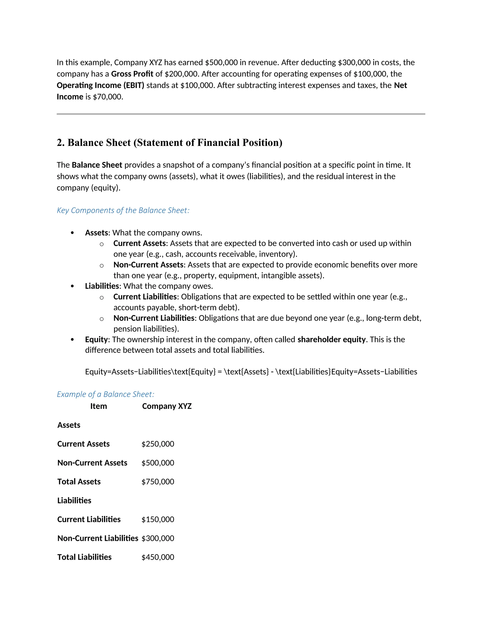
Balance Sheet: In-Depth Explanation
A balance sheet is one of the core financial statements used by businesses to provide a snapshot of their
financial position at a specific point in time. It is sometimes called a statement of financial position
because it provides a detailed summary of a company’s assets, liabilities, and shareholders' equity,
which together must balance according to the accounting equation:
Assets = Liabilities + Shareholders' Equity

20. This equation is at the heart of the balance sheet, reflecting that everything a company owns (assets) is
financed either by borrowing money (liabilities) or by shareholders' investments (equity). The balance
sheet helps stakeholders like investors, creditors, and management understand the company’s financial
health, liquidity, and capital structure.
Components of the Balance Sheet
A typical balance sheet is divided into three main sections: Assets, Liabilities, and Shareholders' Equity.
Each of these categories is then broken down into subcategories to give more detail about the
company's financial structure.
1. Assets
Assets are everything a company owns or controls that has economic value and can be used to generate
future cash flows. Assets are generally classified into two main categories: current assets and non-
current assets.
a. Current Assets
Current assets are assets that are expected to be converted into cash, sold, or consumed within one
year or within the company's normal operating cycle, whichever is longer. These are considered the
most liquid assets because they can be used in the short term to pay for ongoing expenses or
obligations.
 Examples of Current Assets:
o Cash and Cash Equivalents: Money available in bank accounts or short-term
investments.
o Accounts Receivable: Money owed to the company by customers for goods or services
provided on credit.
o Inventory: Goods or raw materials that the company intends to sell or use in its
operations within a year.
o Prepaid Expenses: Payments made for services or goods to be received in the future,
like insurance premiums or rent.
b. Non-Current Assets (Long-Term Assets)
Non-current assets are those that the company expects to hold for more than one year. These assets are
generally less liquid than current assets but are essential for the company's long-term growth and
operations.
 Examples of Non-Current Assets:
o Property, Plant, and Equipment (PPE): Tangible assets like buildings, machinery, and
land used in operations. These assets are typically depreciated over time.

21. o Intangible Assets: Non-physical assets such as patents, trademarks, goodwill, and
intellectual property. These assets are amortized over their useful lives.
o Investments: Long-term investments in other companies or financial assets that the
company plans to hold for more than one year.
2. Liabilities
Liabilities represent a company’s financial obligations or debts—amounts owed to creditors that must
be paid back in the future. Liabilities are similarly divided into current liabilities and non-current
liabilities.
a. Current Liabilities
Current liabilities are obligations the company must settle within one year or within its operating cycle,
whichever is longer.
 Examples of Current Liabilities:
o Accounts Payable: Amounts the company owes to suppliers for goods or services
purchased on credit.
o Short-Term Debt: Loans or borrowings that are due within one year.
o Accrued Expenses: Expenses that have been incurred but not yet paid, such as wages,
taxes, or interest expenses.
o Unearned Revenue: Payments received from customers for goods or services that have
not yet been delivered.
b. Non-Current Liabilities
Non-current liabilities, also known as long-term liabilities, are obligations that the company does not
need to settle within the next year or operating cycle. These are usually paid back over a longer period,
often more than one year.
 Examples of Non-Current Liabilities:
o Long-Term Debt: Loans or bonds payable after one year, such as bank loans or bonds
issued by the company.
o Deferred Tax Liabilities: Taxes owed that are deferred to be paid in the future, usually
due to timing differences between accounting and tax treatments.
o Pension Liabilities: Amounts owed under pension plans or retirement obligations.
3. Shareholders' Equity
Shareholders’ equity (also known as owner’s equity or net worth) represents the residual value of the
company’s assets after all liabilities have been paid. It reflects the ownership interest in the company.
 Examples of Shareholders' Equity:
o Common Stock: The value of shares issued to shareholders, representing ownership in
the company.

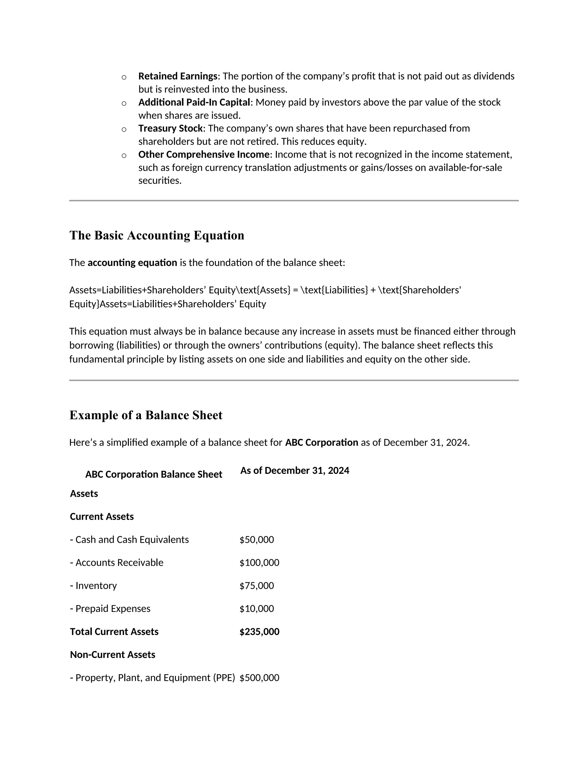
22. o Retained Earnings: The portion of the company’s profit that is not paid out as dividends
but is reinvested into the business.
o Additional Paid-In Capital: Money paid by investors above the par value of the stock
when shares are issued.
o Treasury Stock: The company’s own shares that have been repurchased from
shareholders but are not retired. This reduces equity.
o Other Comprehensive Income: Income that is not recognized in the income statement,
such as foreign currency translation adjustments or gains/losses on available-for-sale
securities.
The Basic Accounting Equation
The accounting equation is the foundation of the balance sheet:
Assets=Liabilities+Shareholders’ Equitytext{Assets} = text{Liabilities} + text{Shareholders'
Equity}Assets=Liabilities+Shareholders’ Equity
This equation must always be in balance because any increase in assets must be financed either through
borrowing (liabilities) or through the owners’ contributions (equity). The balance sheet reflects this
fundamental principle by listing assets on one side and liabilities and equity on the other side.
Example of a Balance Sheet
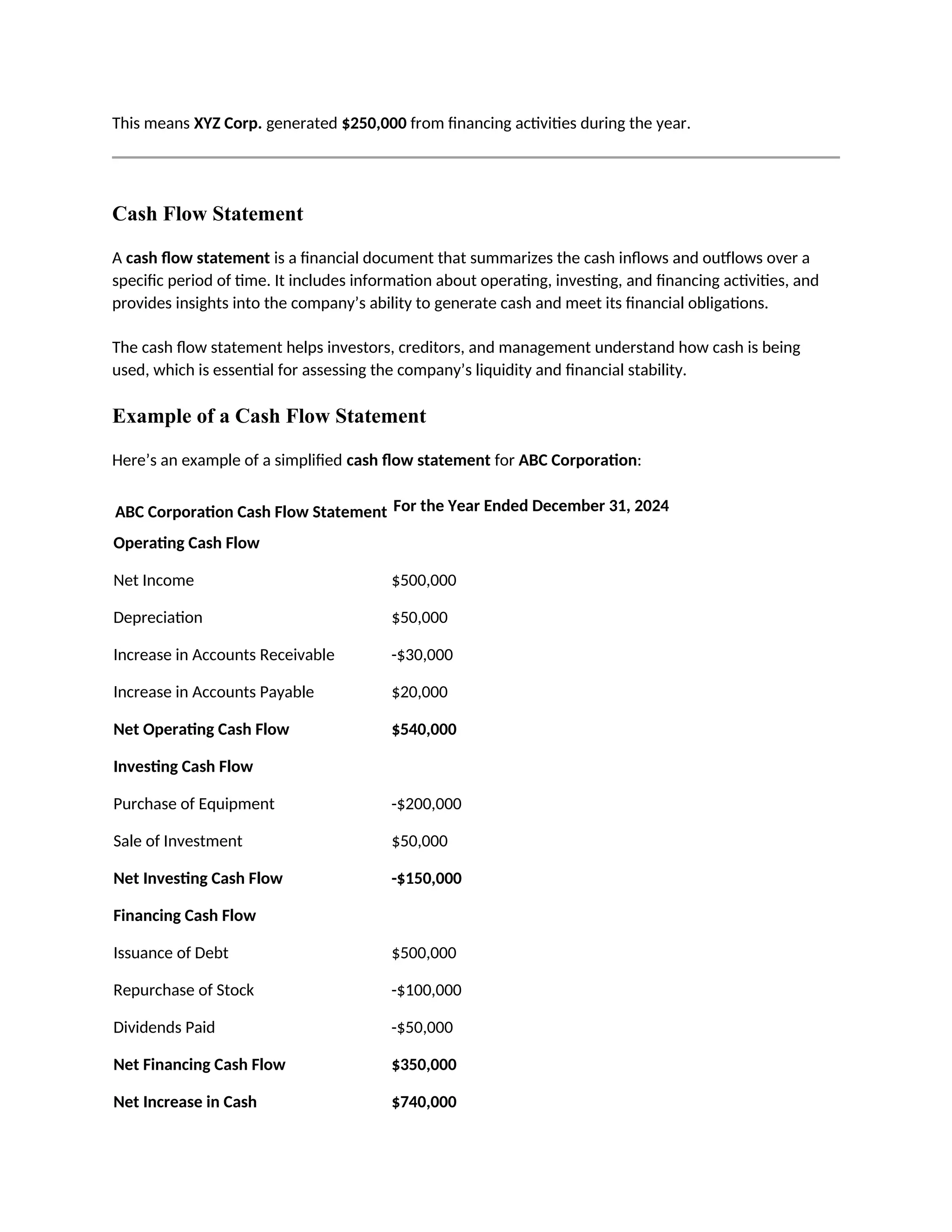
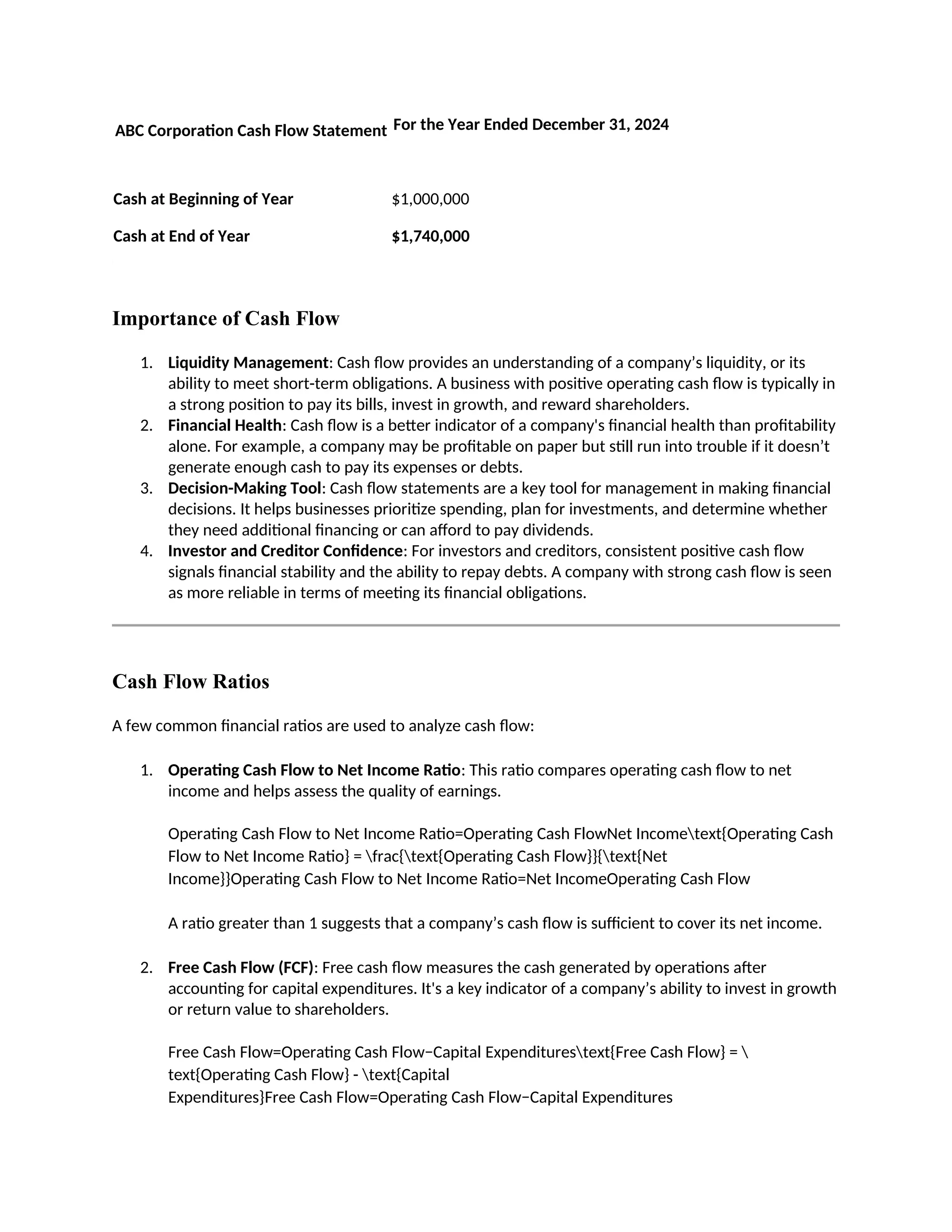
Here’s a simplified example of a balance sheet for ABC Corporation as of December 31, 2024.
ABC Corporation Balance Sheet As of December 31, 2024
Assets
Current Assets
- Cash and Cash Equivalents $50,000
- Accounts Receivable $100,000
- Inventory $75,000
- Prepaid Expenses $10,000
Total Current Assets $235,000
Non-Current Assets
- Property, Plant, and Equipment (PPE) $500,000

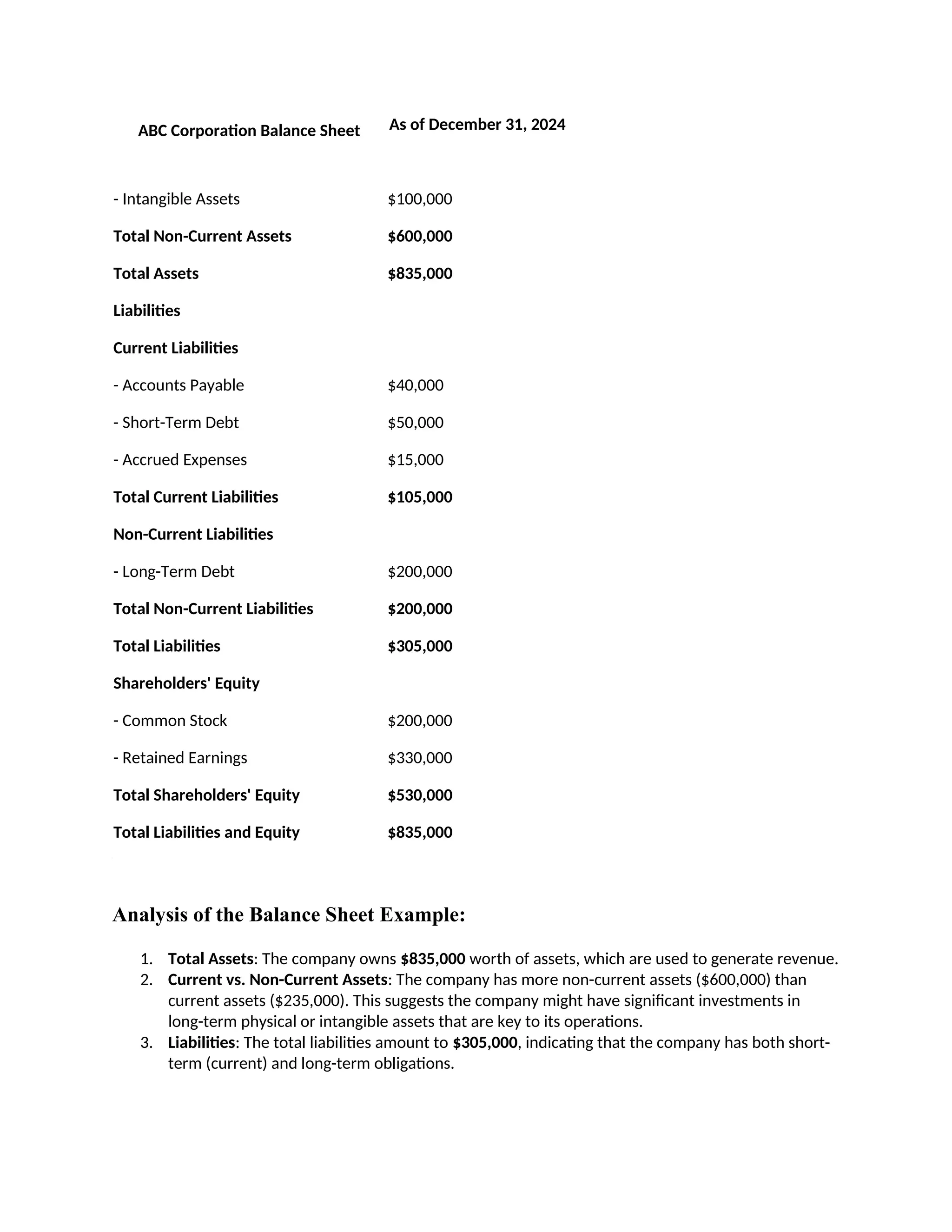
23. ABC Corporation Balance Sheet As of December 31, 2024
- Intangible Assets $100,000
Total Non-Current Assets $600,000
Total Assets $835,000
Liabilities
Current Liabilities
- Accounts Payable $40,000
- Short-Term Debt $50,000
- Accrued Expenses $15,000
Total Current Liabilities $105,000
Non-Current Liabilities
- Long-Term Debt $200,000
Total Non-Current Liabilities $200,000
Total Liabilities $305,000
Shareholders' Equity
- Common Stock $200,000
- Retained Earnings $330,000
Total Shareholders' Equity $530,000
Total Liabilities and Equity $835,000
Analysis of the Balance Sheet Example:
1. Total Assets: The company owns $835,000 worth of assets, which are used to generate revenue.
2. Current vs. Non-Current Assets: The company has more non-current assets ($600,000) than
current assets ($235,000). This suggests the company might have significant investments in
long-term physical or intangible assets that are key to its operations.
3. Liabilities: The total liabilities amount to $305,000, indicating that the company has both short-
term (current) and long-term obligations.

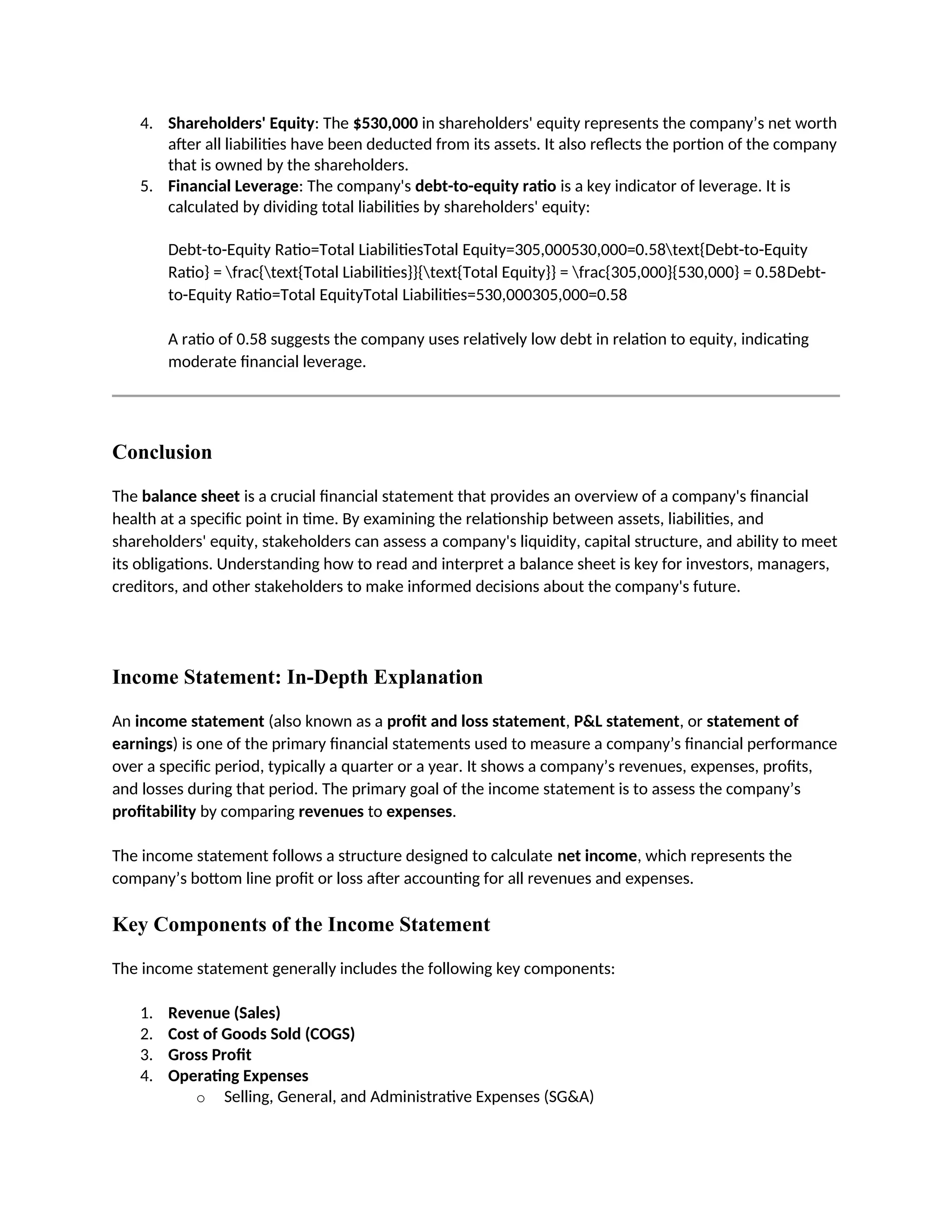
24. 4. Shareholders' Equity: The $530,000 in shareholders' equity represents the company’s net worth
after all liabilities have been deducted from its assets. It also reflects the portion of the company
that is owned by the shareholders.
5. Financial Leverage: The company's debt-to-equity ratio is a key indicator of leverage. It is
calculated by dividing total liabilities by shareholders' equity:
Debt-to-Equity Ratio=Total LiabilitiesTotal Equity=305,000530,000=0.58text{Debt-to-Equity
Ratio} = frac{text{Total Liabilities}}{text{Total Equity}} = frac{305,000}{530,000} = 0.58Debt-
to-Equity Ratio=Total EquityTotal Liabilities=530,000305,000=0.58
A ratio of 0.58 suggests the company uses relatively low debt in relation to equity, indicating
moderate financial leverage.
Conclusion
The balance sheet is a crucial financial statement that provides an overview of a company's financial
health at a specific point in time. By examining the relationship between assets, liabilities, and
shareholders' equity, stakeholders can assess a company's liquidity, capital structure, and ability to meet
its obligations. Understanding how to read and interpret a balance sheet is key for investors, managers,
creditors, and other stakeholders to make informed decisions about the company's future.
Income Statement: In-Depth Explanation
An income statement (also known as a profit and loss statement, P&L statement, or statement of
earnings) is one of the primary financial statements used to measure a company’s financial performance
over a specific period, typically a quarter or a year. It shows a company’s revenues, expenses, profits,
and losses during that period. The primary goal of the income statement is to assess the company’s
profitability by comparing revenues to expenses.
The income statement follows a structure designed to calculate net income, which represents the
company’s bottom line profit or loss after accounting for all revenues and expenses.
Key Components of the Income Statement
The income statement generally includes the following key components:
1. Revenue (Sales)
2. Cost of Goods Sold (COGS)
3. Gross Profit
4. Operating Expenses
o Selling, General, and Administrative Expenses (SG&A)

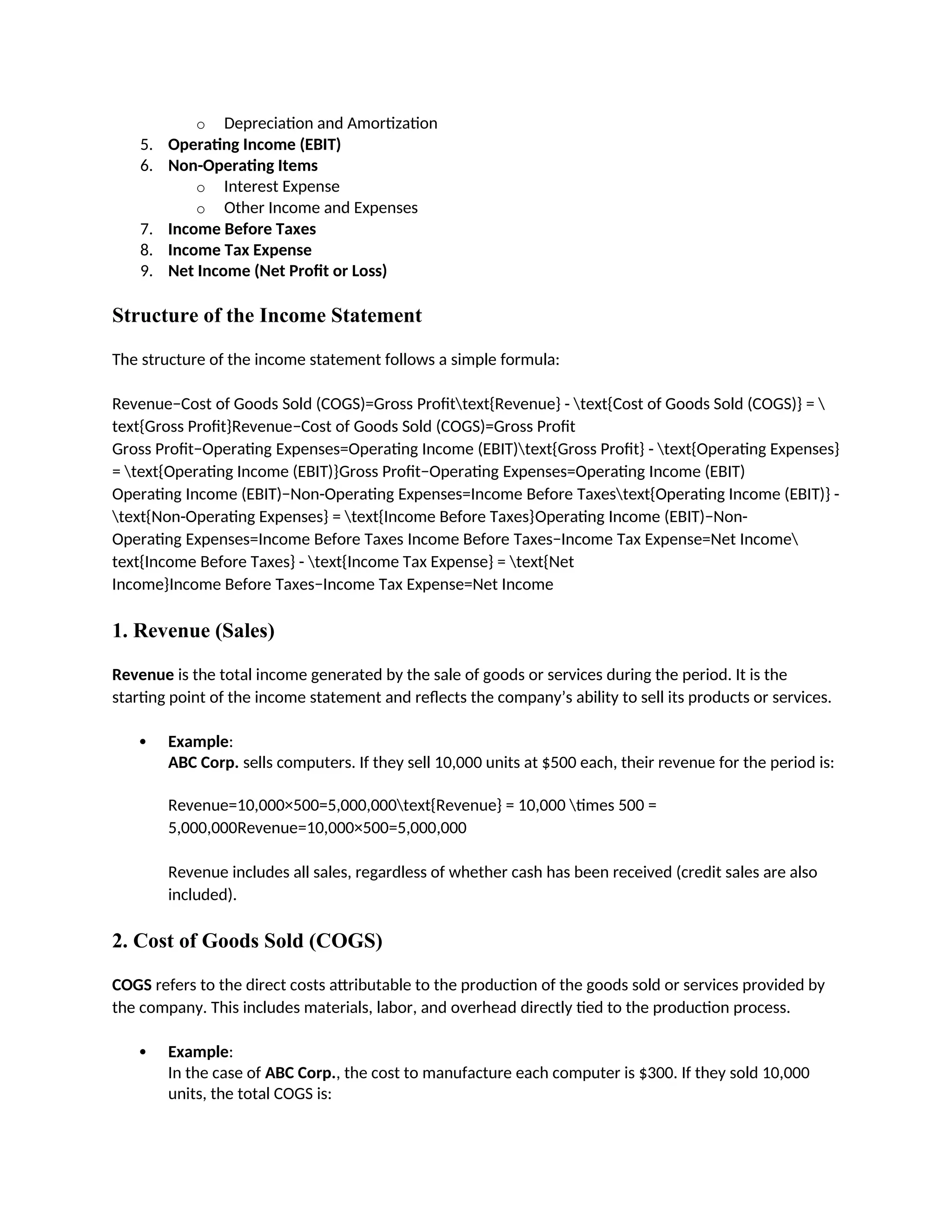
25. o Depreciation and Amortization
5. Operating Income (EBIT)
6. Non-Operating Items
o Interest Expense
o Other Income and Expenses
7. Income Before Taxes
8. Income Tax Expense
9. Net Income (Net Profit or Loss)
Structure of the Income Statement
The structure of the income statement follows a simple formula:
Revenue−Cost of Goods Sold (COGS)=Gross Profittext{Revenue} - text{Cost of Goods Sold (COGS)} =
text{Gross Profit}Revenue−Cost of Goods Sold (COGS)=Gross Profit
Gross Profit−Operating Expenses=Operating Income (EBIT)text{Gross Profit} - text{Operating Expenses}
= text{Operating Income (EBIT)}Gross Profit−Operating Expenses=Operating Income (EBIT)
Operating Income (EBIT)−Non-Operating Expenses=Income Before Taxestext{Operating Income (EBIT)} -
text{Non-Operating Expenses} = text{Income Before Taxes}Operating Income (EBIT)−Non-
Operating Expenses=Income Before Taxes Income Before Taxes−Income Tax Expense=Net Income
text{Income Before Taxes} - text{Income Tax Expense} = text{Net
Income}Income Before Taxes−Income Tax Expense=Net Income
1. Revenue (Sales)
Revenue is the total income generated by the sale of goods or services during the period. It is the
starting point of the income statement and reflects the company’s ability to sell its products or services.
 Example:
ABC Corp. sells computers. If they sell 10,000 units at $500 each, their revenue for the period is:
Revenue=10,000×500=5,000,000text{Revenue} = 10,000 times 500 =
5,000,000Revenue=10,000×500=5,000,000
Revenue includes all sales, regardless of whether cash has been received (credit sales are also
included).
2. Cost of Goods Sold (COGS)
COGS refers to the direct costs attributable to the production of the goods sold or services provided by
the company. This includes materials, labor, and overhead directly tied to the production process.
 Example:
In the case of ABC Corp., the cost to manufacture each computer is $300. If they sold 10,000
units, the total COGS is:

26. COGS=10,000×300=3,000,000text{COGS} = 10,000 times 300 =
3,000,000COGS=10,000×300=3,000,000
3. Gross Profit
Gross profit is the difference between revenue and the cost of goods sold. It measures how efficiently a
company uses its resources (materials and labor) to produce goods or services.
 Formula:
Gross Profit=Revenue−COGStext{Gross Profit} = text{Revenue} -
text{COGS}Gross Profit=Revenue−COGS
 Example:
Continuing with ABC Corp.:
Gross Profit=5,000,000−3,000,000=2,000,000text{Gross Profit} = 5,000,000 - 3,000,000 =
2,000,000Gross Profit=5,000,000−3,000,000=2,000,000
Gross profit reflects the core profitability of the company’s primary business activities.
4. Operating Expenses (OPEX)
Operating expenses are the costs required to run the company on a day-to-day basis. These include
selling, general, and administrative expenses (SG&A), which cover salaries, rent, utilities, marketing,
and other non-production-related expenses.
Depreciation and amortization are also included in operating expenses, as they reflect the allocation of
the cost of tangible and intangible assets over time.
 Example:
ABC Corp. has the following operating expenses:
o SG&A: $700,000
o Depreciation: $100,000 Total operating expenses = $800,000
5. Operating Income (EBIT)
Operating income, also called EBIT (Earnings Before Interest and Taxes), represents the company’s
profit generated from its core operations before accounting for interest and taxes.
 Formula:
Operating Income (EBIT)=Gross Profit−Operating Expensestext{Operating Income (EBIT)} =
text{Gross Profit} - text{Operating
Expenses}Operating Income (EBIT)=Gross Profit−Operating Expenses

27.  Example:
For ABC Corp.:
Operating Income (EBIT)=2,000,000−800,000=1,200,000text{Operating Income (EBIT)} =
2,000,000 - 800,000 = 1,200,000Operating Income (EBIT)=2,000,000−800,000=1,200,000
Operating income is a key measure of a company’s profitability from its regular business
activities.
6. Non-Operating Items
Non-operating items are revenues or expenses that are not directly tied to the core business operations.
These include interest income or expense, gains or losses on asset sales, and other extraordinary items.
Interest Expense:
This is the cost of borrowing money. If a company has debt, it needs to pay interest on that debt, which
reduces its overall profitability.
Other Income/Expenses:
This category includes things like gains or losses on investments, currency fluctuations, or one-time
events.
 Example:
ABC Corp. pays $50,000 in interest on its loans and receives $10,000 in interest income from
investments. The net non-operating income/expense would be:
Net Non-Operating Income=10,000−50,000=−40,000text{Net Non-Operating Income} = 10,000
- 50,000 = -40,000Net Non-Operating Income=10,000−50,000=−40,000
This shows a net expense from non-operating activities.
7. Income Before Taxes
Income before taxes is calculated as operating income plus any non-operating income or minus non-
operating expenses.
 Formula:
Income Before Taxes=Operating Income (EBIT)+Non-Operating Income/Expensetext{Income
Before Taxes} = text{Operating Income (EBIT)} + text{Non-Operating
Income/Expense}Income Before Taxes=Operating Income (EBIT)+Non-Operating Income/
Expense

28.  Example:
For ABC Corp.:
Income Before Taxes=1,200,000−40,000=1,160,000text{Income Before Taxes} = 1,200,000 -
40,000 = 1,160,000Income Before Taxes=1,200,000−40,000=1,160,000
This figure is important as it represents the company’s earnings before it has to pay taxes.
8. Income Tax Expense
This represents the taxes that the company is required to pay based on its taxable income. The tax rate
varies by jurisdiction and the company’s taxable profits.
 Example:
If ABC Corp. is subject to a 30% income tax rate, the tax expense would be:
Income Tax Expense=1,160,000×0.30=348,000text{Income Tax Expense} = 1,160,000 times
0.30 = 348,000Income Tax Expense=1,160,000×0.30=348,000
9. Net Income (Net Profit or Loss)
Finally, net income represents the company’s final profit or loss after all expenses, including taxes, have
been deducted from total revenues. It is often referred to as the bottom line of the income statement,
as it reflects the overall profitability of the company.
 Formula:
Net Income=Income Before Taxes−Income Tax Expensetext{Net Income} = text{Income Before
Taxes} - text{Income Tax Expense}Net Income=Income Before Taxes−Income Tax Expense
 Example:
For ABC Corp.:
Net Income=1,160,000−348,000=812,000text{Net Income} = 1,160,000 - 348,000 =
812,000Net Income=1,160,000−348,000=812,000
Net income is a key measure of the company’s profitability and is used by investors, creditors,
and management to evaluate financial performance.
Example of a Full Income Statement
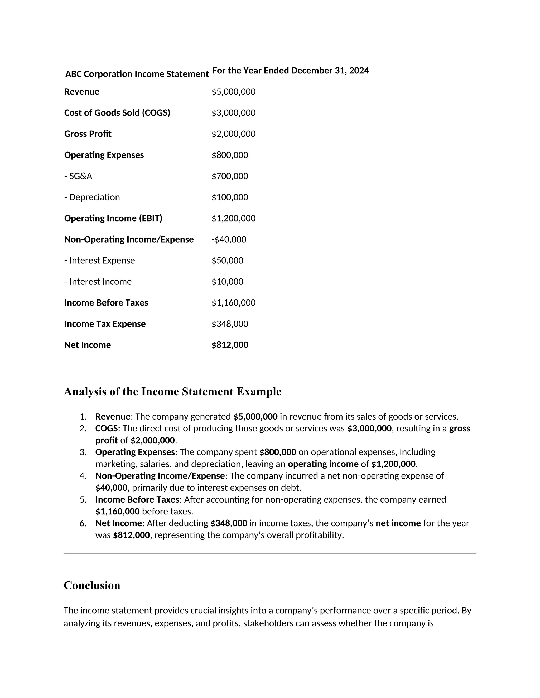
Here’s an example of a complete income statement for ABC Corporation for the year ended December
31, 2024:

29. ABC Corporation Income Statement For the Year Ended December 31, 2024
Revenue $5,000,000
Cost of Goods Sold (COGS) $3,000,000
Gross Profit $2,000,000
Operating Expenses $800,000
- SG&A $700,000
- Depreciation $100,000
Operating Income (EBIT) $1,200,000
Non-Operating Income/Expense -$40,000
- Interest Expense $50,000
- Interest Income $10,000
Income Before Taxes $1,160,000
Income Tax Expense $348,000
Net Income $812,000
Analysis of the Income Statement Example
1. Revenue: The company generated $5,000,000 in revenue from its sales of goods or services.
2. COGS: The direct cost of producing those goods or services was $3,000,000, resulting in a gross
profit of $2,000,000.
3. Operating Expenses: The company spent $800,000 on operational expenses, including
marketing, salaries, and depreciation, leaving an operating income of $1,200,000.
4. Non-Operating Income/Expense: The company incurred a net non-operating expense of
$40,000, primarily due to interest expenses on debt.
5. Income Before Taxes: After accounting for non-operating expenses, the company earned
$1,160,000 before taxes.
6. Net Income: After deducting $348,000 in income taxes, the company’s net income for the year
was $812,000, representing the company’s overall profitability.
Conclusion
The income statement provides crucial insights into a company’s performance over a specific period. By
analyzing its revenues, expenses, and profits, stakeholders can assess whether the company is

30. effectively managing its costs, growing its sales, and generating sufficient profit. The net income figure at
the bottom of the statement is one of the most important indicators of financial health, and it plays a
key role in decision-making by investors, creditors, and company management.
Taxes: In-Depth Explanation
Taxes are mandatory financial charges or levies imposed by governments on individuals, businesses, and
other entities to fund government expenditures, such as public services, infrastructure, and defense.
They are a central element of the economic system, as they allow governments to raise revenue for
various programs and services that benefit society.
Taxes can take many forms, ranging from income taxes to sales taxes, property taxes, and corporate
taxes. Understanding taxes is essential for both individuals and businesses, as they impact financial
decisions, income, and profitability.
Types of Taxes
Taxes are categorized into several types, primarily based on their nature and the entities they apply to.
Below are the major types of taxes:
1. Income Taxes
Income taxes are taxes levied on the earnings of individuals or businesses. Governments typically
impose a progressive income tax system, where higher income is taxed at higher rates.
a. Individual Income Tax
This is the tax on personal income, which includes wages, salaries, interest, dividends, capital gains, and
other sources of income.
 Example:
Suppose an individual earns $100,000 annually. If the tax rate is 20% on income up to $50,000,
and 30% on income above that, the tax would be calculated as:
text{Tax on First $50,000} = 50,000 times 0.20 = 10,000 text{Tax on Remaining $50,000} =
50,000 times 0.30 = 15,000 Total Income Tax=10,000+15,000=25,000text{Total Income Tax} =
10,000 + 15,000 = 25,000Total Income Tax=10,000+15,000=25,000
The individual would owe $25,000 in income tax.

31. b. Corporate Income Tax
Businesses also pay income taxes on their profits. The corporate income tax rate can vary by country
and is typically a fixed percentage of net income.
 Example:
A corporation earns $1,000,000 in profit for the year. If the corporate tax rate is 25%, the
company would owe:
Corporate Tax=1,000,000×0.25=250,000text{Corporate Tax} = 1,000,000 times 0.25 =
250,000Corporate Tax=1,000,000×0.25=250,000
The corporation would pay $250,000 in income taxes.
2. Sales Tax
Sales tax is a consumption tax placed on the sale of goods and services. Typically, it is a percentage of
the sale price and is paid by the buyer, although businesses collect it and remit it to the government.
 Example:
If a state imposes a sales tax rate of 8% and you purchase a $100 item, the sales tax would be:
Sales Tax=100×0.08=8text{Sales Tax} = 100 times 0.08 = 8Sales Tax=100×0.08=8
You would pay a total of $108 for the item, which includes the $8 sales tax.
3. Property Tax
Property taxes are levied on property owners, typically based on the value of their property (real
estate). This includes both land and buildings.
 Example:
If a property is valued at $500,000 and the local government imposes a property tax rate of
1.5%, the tax would be:
Property Tax=500,000×0.015=7,500text{Property Tax} = 500,000 times 0.015 =
7,500Property Tax=500,000×0.015=7,500
The property owner would pay $7,500 in property taxes annually.

32. 4. Payroll Taxes
Payroll taxes are taxes withheld from an employee's wages and used to fund social insurance programs
like Social Security, Medicare, and unemployment insurance.
a. Social Security and Medicare Taxes (FICA Taxes)
In the U.S., the Federal Insurance Contributions Act (FICA) requires employers to withhold social security
and Medicare taxes from employees' paychecks.
 Example:
If an employee earns $60,000 annually, the total FICA tax rate (for Social Security and Medicare)
is 7.65%, split into 6.2% for Social Security and 1.45% for Medicare.
The tax would be calculated as:
FICA Tax=60,000×0.0765=4,590text{FICA Tax} = 60,000 times 0.0765 =
4,590FICA Tax=60,000×0.0765=4,590
The employee would owe $4,590 in payroll taxes for the year, which is withheld by the
employer and paid to the government.
5. Capital Gains Tax
Capital gains tax is levied on the profits from the sale of assets such as stocks, bonds, and real estate.
The rate varies based on the holding period (short-term vs. long-term) and the individual's tax bracket.
a. Short-Term Capital Gains Tax
If an asset is held for one year or less before being sold, the gain is considered short-term and is taxed at
the individual’s ordinary income tax rate.
b. Long-Term Capital Gains Tax
If the asset is held for more than one year, the gain is subject to a lower long-term capital gains tax rate.
 Example:
If you sell an investment for $10,000 that you purchased for $7,000, your capital gain is $3,000.
If the long-term capital gains tax rate is 15%, the tax owed would be:
Capital Gains Tax=3,000×0.15=450text{Capital Gains Tax} = 3,000 times 0.15 =
450Capital Gains Tax=3,000×0.15=450
You would owe $450 in capital gains taxes.

33. 6. Estate and Inheritance Taxes
Estate taxes are taxes imposed on the transfer of an estate upon an individual's death. Inheritance taxes
are taxes on the value of the assets inherited by heirs.
 Example:
If a person inherits $1,000,000 from a deceased relative and the inheritance tax rate is 10%, the
heir would owe:
Inheritance Tax=1,000,000×0.10=100,000text{Inheritance Tax} = 1,000,000 times 0.10 =
100,000Inheritance Tax=1,000,000×0.10=100,000
The heir would pay $100,000 in inheritance taxes.
Taxation Systems
Different countries and regions employ different taxation systems. The key systems are:
1. Progressive Taxation
In a progressive tax system, the tax rate increases as the taxable amount increases. This is typically seen
in personal income taxes, where individuals with higher incomes are taxed at higher rates.
 Example:
In a progressive tax system, if an individual earns $50,000, they may be taxed at a rate of 10%,
whereas someone earning $200,000 might be taxed at a rate of 30%.
2. Regressive Taxation
In a regressive tax system, the tax rate decreases as the taxable amount increases. This is commonly
seen in sales taxes, where the percentage remains constant but the relative impact is larger on lower-
income individuals because they spend a higher portion of their income on taxed goods.
 Example:
A 10% sales tax on a $100 purchase is a smaller burden for a wealthy individual than for
someone with a lower income, as the tax is a larger percentage of their income.
3. Proportional (Flat) Taxation
In a flat tax system, everyone is taxed at the same rate, regardless of income level. This is often seen in
corporate taxes or certain individual income tax systems.

34.  Example:
If a country implements a flat tax rate of 15%, both a person earning $50,000 and a person
earning $500,000 would pay the same percentage of their income in taxes.
International Tax Considerations
Multinational companies and individuals with assets in multiple countries may be subject to double
taxation, where both their home country and the country in which they operate tax their income. To
avoid this, many countries enter into tax treaties to reduce or eliminate double taxation.
 Example:
A U.S.-based company operating in Europe may pay taxes to both the U.S. and the European
country. However, due to tax treaties, the company might receive a tax credit or exemption to
avoid being taxed twice on the same income.
Tax Avoidance vs. Tax Evasion
 Tax Avoidance:
Tax avoidance is the legal practice of minimizing taxes by taking advantage of deductions,
credits, and other strategies. It's legal and often involves strategic planning to reduce tax
liabilities.
o Example:
A company might claim deductions for business expenses like office supplies, travel, and
depreciation to reduce its taxable income.
 Tax Evasion:
Tax evasion is the illegal act of deliberately falsifying tax information or hiding income to avoid
paying taxes. It’s considered a crime and can lead to fines and penalties.
o Example:
A business might hide revenue from sales to avoid paying sales tax or underreport
income to reduce income tax obligations.
Conclusion
Taxes are essential for financing government functions and services, but they can be complex. Different
types of taxes, such as income taxes, sales taxes, and property taxes, affect individuals and businesses in
various ways. Understanding the intricacies of the tax system is important for making informed financial
decisions and ensuring compliance with tax laws. While tax avoidance strategies can help minimize
liabilities legally, tax evasion can result in significant penalties and legal consequences.

35. Cash Flow: In-Depth Explanation
Cash flow refers to the movement of money into and out of a business over a specific period of time. It
is an essential measure of a company's financial health and liquidity, showing how much cash a business
generates or spends from its operations, investments, and financing activities. Cash flow is crucial
because even a profitable business can face financial difficulties if it does not manage its cash flow
effectively.
The primary goal of cash flow analysis is to ensure that a business can meet its obligations, such as
paying bills, repaying loans, and funding growth, while also maintaining enough liquidity to continue
operations.
Types of Cash Flow
Cash flow is typically broken down into three main categories, reflecting the different sources of cash
inflows and outflows:
1. Operating Cash Flow (OCF)
2. Investing Cash Flow (ICF)
3. Financing Cash Flow (FCF)
1. Operating Cash Flow (OCF)
Operating cash flow is the cash generated or used by a company's core business activities. It represents
the net cash generated from the company’s day-to-day operations, excluding any investments or
financing activities.
Operating cash flow can be calculated using two methods:
 Direct method: Lists all cash inflows and outflows from operating activities.
 Indirect method: Starts with net income and adjusts for changes in working capital and non-
cash items like depreciation.
Key Components of Operating Cash Flow:
 Cash Receipts from Customers: Cash inflows from the sale of goods or services.
 Cash Payments to Suppliers: Cash outflows related to the production or acquisition of goods or
services.

36.  Operating Expenses: Cash outflows for wages, rent, utilities, etc.
 Interest and Taxes: Cash payments related to interest on debt and taxes.
Example of Operating Cash Flow:
Let's assume XYZ Corp. reports the following activities for a quarter:
 Revenue: $500,000 from sales to customers.
 Payments to Suppliers: $200,000 for inventory and materials.
 Operating Expenses: $100,000 in wages, rent, and utilities.
 Interest Payments: $20,000.
 Taxes: $30,000.
The operating cash flow can be calculated as follows:
Operating Cash Flow=Cash Receipts from Customers−Cash Payments to Suppliers−Operating Expenses−I
nterest Payments−Taxes Paidtext{Operating Cash Flow} = text{Cash Receipts from Customers} -
text{Cash Payments to Suppliers} - text{Operating Expenses} - text{Interest Payments} - text{Taxes
Paid}Operating Cash Flow=Cash Receipts from Customers−Cash Payments to Suppliers−Operating Expen
ses−Interest Payments−Taxes Paid
Operating Cash Flow=500,000−200,000−100,000−20,000−30,000=150,000text{Operating Cash Flow} =
500,000 - 200,000 - 100,000 - 20,000 - 30,000 =
150,000Operating Cash Flow=500,000−200,000−100,000−20,000−30,000=150,000
This means XYZ Corp. generated $150,000 in cash from its core operations for the quarter.
2. Investing Cash Flow (ICF)
Investing cash flow refers to the cash inflows and outflows associated with the acquisition and disposal
of long-term assets, such as property, equipment, or securities. It represents investments made by the
company in its future growth or returns.
Key Components of Investing Cash Flow:
 Purchases of Property, Plant, and Equipment (Capex): Cash outflows for purchasing long-term
assets.
 Proceeds from the Sale of Assets: Cash inflows from selling property, equipment, or
investments.
 Investments in Securities: Cash outflows or inflows related to buying or selling investments.
Example of Investing Cash Flow:
Let's assume ABC Corp. made the following investments during the year:

37.  Purchased Equipment: $200,000.
 Sold Property: $50,000.
 Invested in Stocks: $30,000.
The investing cash flow is calculated as:
Investing Cash Flow=Proceeds from Sales−Purchases of Assets−Investments in Securitiestext{Investing
Cash Flow} = text{Proceeds from Sales} - text{Purchases of Assets} - text{Investments in
Securities}Investing Cash Flow=Proceeds from Sales−Purchases of Assets−Investments in Securities
Investing Cash Flow=50,000−200,000−30,000=−180,000text{Investing Cash Flow} = 50,000 - 200,000 -
30,000 = -180,000Investing Cash Flow=50,000−200,000−30,000=−180,000
This means ABC Corp. had a net outflow of $180,000 in investing activities during the year.
3. Financing Cash Flow (FCF)
Financing cash flow refers to the cash movements between a company and its creditors and
shareholders. It includes cash inflows from issuing debt or equity, and cash outflows from repaying debt
or distributing dividends.
Key Components of Financing Cash Flow:
 Issuance of Debt or Equity: Cash inflows from borrowing or selling shares.
 Repayment of Debt: Cash outflows from repaying loans or bonds.
 Dividend Payments: Cash outflows related to dividends paid to shareholders.
Example of Financing Cash Flow:
Let's assume XYZ Corp. engaged in the following financing activities during the year:
 Issued New Debt: $500,000.
 Repurchased Stock: $150,000.
 Paid Dividends: $100,000.
The financing cash flow would be calculated as:
Financing Cash Flow=Proceeds from Issuing Debt−Repurchase of Stock−Dividend Payments
text{Financing Cash Flow} = text{Proceeds from Issuing Debt} - text{Repurchase of Stock} -
text{Dividend
Payments}Financing Cash Flow=Proceeds from Issuing Debt−Repurchase of Stock−Dividend Payments
Financing Cash Flow=500,000−150,000−100,000=250,000text{Financing Cash Flow} = 500,000 - 150,000
- 100,000 = 250,000Financing Cash Flow=500,000−150,000−100,000=250,000

38. This means XYZ Corp. generated $250,000 from financing activities during the year.
Cash Flow Statement
A cash flow statement is a financial document that summarizes the cash inflows and outflows over a
specific period of time. It includes information about operating, investing, and financing activities, and
provides insights into the company’s ability to generate cash and meet its financial obligations.
The cash flow statement helps investors, creditors, and management understand how cash is being
used, which is essential for assessing the company’s liquidity and financial stability.
Example of a Cash Flow Statement
Here’s an example of a simplified cash flow statement for ABC Corporation:
ABC Corporation Cash Flow Statement For the Year Ended December 31, 2024
Operating Cash Flow
Net Income $500,000
Depreciation $50,000
Increase in Accounts Receivable -$30,000
Increase in Accounts Payable $20,000
Net Operating Cash Flow $540,000
Investing Cash Flow
Purchase of Equipment -$200,000
Sale of Investment $50,000
Net Investing Cash Flow -$150,000
Financing Cash Flow
Issuance of Debt $500,000
Repurchase of Stock -$100,000
Dividends Paid -$50,000
Net Financing Cash Flow $350,000
Net Increase in Cash $740,000

39. ABC Corporation Cash Flow Statement For the Year Ended December 31, 2024
Cash at Beginning of Year $1,000,000
Cash at End of Year $1,740,000
Importance of Cash Flow
1. Liquidity Management: Cash flow provides an understanding of a company’s liquidity, or its
ability to meet short-term obligations. A business with positive operating cash flow is typically in
a strong position to pay its bills, invest in growth, and reward shareholders.
2. Financial Health: Cash flow is a better indicator of a company's financial health than profitability
alone. For example, a company may be profitable on paper but still run into trouble if it doesn’t
generate enough cash to pay its expenses or debts.
3. Decision-Making Tool: Cash flow statements are a key tool for management in making financial
decisions. It helps businesses prioritize spending, plan for investments, and determine whether
they need additional financing or can afford to pay dividends.
4. Investor and Creditor Confidence: For investors and creditors, consistent positive cash flow
signals financial stability and the ability to repay debts. A company with strong cash flow is seen
as more reliable in terms of meeting its financial obligations.
Cash Flow Ratios
A few common financial ratios are used to analyze cash flow:
1. Operating Cash Flow to Net Income Ratio: This ratio compares operating cash flow to net
income and helps assess the quality of earnings.
Operating Cash Flow to Net Income Ratio=Operating Cash FlowNet Incometext{Operating Cash
Flow to Net Income Ratio} = frac{text{Operating Cash Flow}}{text{Net
Income}}Operating Cash Flow to Net Income Ratio=Net IncomeOperating Cash Flow
A ratio greater than 1 suggests that a company’s cash flow is sufficient to cover its net income.
2. Free Cash Flow (FCF): Free cash flow measures the cash generated by operations after
accounting for capital expenditures. It's a key indicator of a company’s ability to invest in growth
or return value to shareholders.
Free Cash Flow=Operating Cash Flow−Capital Expenditurestext{Free Cash Flow} =
text{Operating Cash Flow} - text{Capital
Expenditures}Free Cash Flow=Operating Cash Flow−Capital Expenditures

40. Example: If a company has $500,000 in operating cash flow and $150,000 in capital
expenditures, its free cash flow is:
Free Cash Flow=500,000−150,000=350,000text{Free Cash Flow} = 500,000 - 150,000 =
350,000Free Cash Flow=500,000−150,000=350,000
3. Cash Flow Margin: This ratio measures the percentage of revenue that is converted into cash
flow from operations.
Cash Flow Margin=Operating Cash FlowRevenuetext{Cash Flow Margin} = frac{text{Operating
Cash Flow}}{text{Revenue}}Cash Flow Margin=RevenueOperating Cash Flow
Example: If a company has $1,000,000 in revenue and $200,000 in operating cash flow, the cash
flow margin is:
text{Cash Flow Margin} = frac{200,000}{1,000,000} = 0.20 text{ or 20%}
Conclusion
Cash flow is a critical indicator of a company’s financial health, and understanding how cash flows in and
out of the business is essential for effective decision-making. By analyzing cash flow from operations,
investments, and financing activities, a business can ensure that it has the liquidity to meet obligations,
invest in growth, and achieve long-term success.
Standardizing financial statements is a crucial practice in accounting and financial analysis. It
ensures consistency, comparability, and transparency in financial reporting, making it easier to
analyze the financial health of a business, compare companies within the same industry, and
assess overall performance. Below is an in-depth explanation of standardizing financial
statements, including examples.
What is Standardization of Financial Statements?
Standardizing financial statements means adjusting financial data in a way that makes it easier to
compare across companies, periods, or industries. The main goal is to eliminate inconsistencies
that can arise from differences in accounting policies, company size, or operational structures.
By standardizing, you transform financial figures into relative numbers (ratios, percentages, or
per-unit figures), making it easier to assess a company’s performance regardless of its size or the
period under review.
Types of Standardized Financial Statements

41. 1. Common-Size Financial Statements:
Common-size financial statements present each line item as a percentage of a key figure
such as sales (in the income statement) or total assets (in the balance sheet).
o Common-Size Income Statement: Each item is expressed as a percentage of
total sales (revenue).
o Common-Size Balance Sheet: Each item is expressed as a percentage of total
assets.
Example:
For an income statement, you might have the following figures (in millions):
o Revenue: $1,000
o Cost of Goods Sold (COGS): $600
o Operating Profit: $200
o Net Profit: $100
To standardize, you calculate the percentage of each item in relation to revenue:
o Revenue = $1,000 (100%)
o COGS = $600 (60%)
o Operating Profit = $200 (20%)
o Net Profit = $100 (10%)
This allows for comparison between companies of different sizes. For example, if another
company has $5,000 in revenue, and its COGS is $3,000, its COGS percentage would be
60%, the same as the first company, making it easy to compare their cost structures.
2. Ratio Analysis:
Ratio analysis uses financial ratios derived from standardized data to assess a company's
performance. These ratios typically include profitability, liquidity, efficiency, and
solvency ratios.
Common ratios include:
o Current Ratio: Current Assets / Current Liabilities
o Quick Ratio: (Current Assets - Inventory) / Current Liabilities
o Return on Equity (ROE): Net Income / Shareholders' Equity
o Net Profit Margin: Net Income / Revenue
Example:
For a company with the following figures:
o Net Income = $100,000
o Revenue = $500,000
o Shareholders' Equity = $1,000,000

42. The Net Profit Margin would be:
Net Profit Margin=Net IncomeRevenue=100,000500,000=0.20 or 20%text{Net Profit
Margin} = frac{text{Net Income}}{text{Revenue}} = frac{100,000}{500,000} =
0.20 text{ or } 20%Net Profit Margin=RevenueNet Income=500,000100,000
=0.20 or 20%
3. Trend Analysis:
This involves comparing financial data over a series of periods to identify patterns and
trends. Standardizing the data, such as converting each figure to a base year or
percentage, allows for clear trend identification.
Example:
If a company's revenue has grown from $800,000 in 2020 to $1,200,000 in 2024, you can
standardize by taking the base year (2020) as 100%:
o 2020: $800,000 (100%)
o 2021: $900,000 (112.5%)
o 2022: $1,000,000 (125%)
o 2023: $1,100,000 (137.5%)
o 2024: $1,200,000 (150%)
This makes it easy to see that the company has grown its revenue by 50% from 2020 to
2024.
4. Industry Benchmarking:
Standardization allows companies to compare their financial performance to industry
averages or best practices. Ratios like Return on Assets (ROA), Return on Equity
(ROE), or Debt-to-Equity ratio can be compared against industry standards or peer
companies.
Example:
o A company has a ROE of 18%.
o The industry average is 15%.
o This indicates that the company is performing better than the industry in terms of
generating profit for every dollar of equity.
5. Inflation Adjustment:
In some cases, it may be necessary to adjust financial statements for inflation to ensure
that the real value of assets and income is being measured, especially when comparing
figures from different periods. This is commonly done in countries with high inflation
rates or when comparing long-term historical data.
Example:
Suppose you are comparing the revenue of a company in 1990 ($100,000) and 2020

43. ($500,000). If inflation between these years was 200%, the 1990 revenue adjusted for
inflation would be:
100,000×(1+2)=300,000100,000 times (1 + 2) = 300,000100,000×(1+2)=300,000
This gives a better sense of the company’s growth in real terms, rather than nominal
figures.
Advantages of Standardizing Financial Statements
1. Enhanced Comparability:
Standardized financial statements allow investors, analysts, and managers to compare
companies of different sizes and in different sectors more easily.
2. Better Performance Evaluation:
By standardizing the data, you can better assess how well a company is performing
relative to its peers or its historical performance.
3. Improved Decision-Making:
Investors and management can make better-informed decisions when they have clear,
standardized data that shows trends, risks, and opportunities.
4. Identification of Financial Strengths and Weaknesses:
Standardized financial ratios and metrics help to pinpoint areas where the company is
doing well and where it might need improvement.
Conclusion
Standardizing financial statements is an essential part of financial analysis, making it easier to
compare companies, assess performance, and identify trends. By using methods such as
common-size statements, ratio analysis, and trend analysis, businesses, analysts, and investors
can gain valuable insights into a company's financial health and make more informed decisions.
Would you like me to help you standardize a particular set of financial statements, or would you
like further examples of any of the methods mentioned?
Analyzing financial statements in depth is a key practice for assessing the financial health and
performance of a business. This process involves reviewing and interpreting a company’s financial
statements, including the balance sheet, income statement, and cash flow statement, to gain insights
into its profitability, liquidity, solvency, and efficiency.
In-depth financial statement analysis allows investors, creditors, and managers to understand not just
what has happened in the past, but also to predict future performance and identify areas for
improvement.
Here’s an in-depth guide to analyzing financial statements, along with examples:

44. 1. Balance Sheet Analysis
The balance sheet provides a snapshot of a company's assets, liabilities, and equity at a specific point in
time. The basic formula is:
Assets=Liabilities+Equitytext{Assets} = text{Liabilities} + text{Equity}Assets=Liabilities+Equity
Key Elements of the Balance Sheet:
 Assets: Everything the company owns. These are usually divided into:
o Current Assets (e.g., cash, receivables, inventory)
o Non-current Assets (e.g., property, plant, equipment, intangible assets)
 Liabilities: Everything the company owes. These are divided into:
o Current Liabilities (e.g., short-term debt, accounts payable)
o Non-current Liabilities (e.g., long-term debt, pension obligations)
 Equity: The residual interest in the assets after deducting liabilities. This includes:
o Common Stock
o Retained Earnings
o Additional Paid-in Capital
Key Ratios for Balance Sheet Analysis:
 Current Ratio: Measures liquidity by comparing current assets to current liabilities.
Current Ratio=Current AssetsCurrent Liabilitiestext{Current Ratio} = frac{text{Current Assets}}
{text{Current Liabilities}}Current Ratio=Current LiabilitiesCurrent Assets
A ratio above 1 indicates that the company can cover its short-term obligations with its short-
term assets.
Example:
o Current Assets = $500,000
o Current Liabilities = $300,000
Current Ratio=500,000300,000=1.67text{Current Ratio} = frac{500,000}{300,000} =
1.67Current Ratio=300,000500,000=1.67
A current ratio of 1.67 suggests the company is in a good position to meet its short-term
obligations.
 Debt-to-Equity Ratio: Measures the company’s leverage by comparing its total liabilities to its
shareholders' equity.
Debt-to-Equity Ratio=Total LiabilitiesTotal Equitytext{Debt-to-Equity Ratio} = frac{text{Total
Liabilities}}{text{Total Equity}}Debt-to-Equity Ratio=Total EquityTotal Liabilities

45. A higher ratio indicates more debt relative to equity, which can be risky but also leverage
growth.
Example:
o Total Liabilities = $1,200,000
o Total Equity = $800,000
Debt-to-Equity Ratio=1,200,000800,000=1.5text{Debt-to-Equity Ratio} = frac{1,200,000}
{800,000} = 1.5Debt-to-Equity Ratio=800,0001,200,000=1.5
A debt-to-equity ratio of 1.5 means the company has 1.5 times more debt than equity.
2. Income Statement Analysis
The income statement (or profit and loss statement) summarizes a company’s revenue, expenses, and
profits over a period (usually quarterly or annually). It helps you understand the company’s profitability.
Key Elements of the Income Statement:
 Revenue/Sales: The total income from the company’s core operations.
 Cost of Goods Sold (COGS): Direct costs of producing the goods sold or services provided.
 Gross Profit: Revenue minus COGS.
 Operating Expenses: Costs associated with running the business, such as rent, salaries, and
marketing.
 Operating Income (EBIT): Gross profit minus operating expenses.
 Net Income: The company’s total profit after all expenses, taxes, and interest are deducted.
Key Ratios for Income Statement Analysis:
 Gross Profit Margin: Indicates the percentage of revenue that exceeds the cost of goods sold.
Gross Profit Margin=Gross ProfitRevenue×100text{Gross Profit Margin} = frac{text{Gross
Profit}}{text{Revenue}} times 100Gross Profit Margin=RevenueGross Profit×100
A higher gross profit margin indicates more efficient production or service delivery.
Example:
o Revenue = $1,000,000
o COGS = $600,000
Gross Profit Margin=1,000,000−600,0001,000,000×100=40%text{Gross Profit Margin} =
frac{1,000,000 - 600,000}{1,000,000} times 100 =
40%Gross Profit Margin=1,000,0001,000,000−600,000×100=40%

46. A gross profit margin of 40% suggests the company is retaining 40% of its revenue after
covering direct costs.
 Net Profit Margin: Measures how much of each dollar of revenue results in profit after all
expenses.
Net Profit Margin=Net IncomeRevenue×100text{Net Profit Margin} = frac{text{Net Income}}{
text{Revenue}} times 100Net Profit Margin=RevenueNet Income×100
Example:
o Net Income = $100,000
o Revenue = $1,000,000
Net Profit Margin=100,0001,000,000×100=10%text{Net Profit Margin} = frac{100,000}
{1,000,000} times 100 = 10%Net Profit Margin=1,000,000100,000×100=10%
A net profit margin of 10% means the company earns 10 cents in profit for every dollar of
revenue.
 Earnings Before Interest and Taxes (EBIT): Measures the company’s profitability from
operations, ignoring interest and taxes.
Example:
If operating income is $200,000, and the company pays $50,000 in interest and $20,000 in taxes,
its EBIT would be:
EBIT=200,000text{EBIT} = 200,000EBIT=200,000
3. Cash Flow Statement Analysis
The cash flow statement shows how cash is flowing in and out of the company, categorizing activities
into:
 Operating Activities: Cash generated or used by the core business activities.
 Investing Activities: Cash used for or generated from investments in long-term assets.
 Financing Activities: Cash received from or paid to investors and creditors (e.g., issuing stock,
borrowing, repaying debt).
Key Ratios for Cash Flow Analysis:
 Operating Cash Flow to Net Income: Measures the quality of earnings by comparing cash flow
from operations to net income.

47. Operating Cash Flow to Net Income=Operating Cash FlowNet Incometext{Operating Cash Flow
to Net Income} = frac{text{Operating Cash Flow}}{text{Net
Income}}Operating Cash Flow to Net Income=Net IncomeOperating Cash Flow
A ratio above 1 suggests strong cash generation from operations.
Example:
o Operating Cash Flow = $150,000
o Net Income = $100,000
Operating Cash Flow to Net Income=150,000100,000=1.5text{Operating Cash Flow to Net
Income} = frac{150,000}{100,000} = 1.5Operating Cash Flow to Net Income=100,000150,000
=1.5
A ratio of 1.5 suggests that the company’s net income is well supported by cash flow.
 Free Cash Flow (FCF): Represents the cash a company generates after capital expenditures,
available for distribution to investors.
Free Cash Flow=Operating Cash Flow−Capital Expenditurestext{Free Cash Flow} =
text{Operating Cash Flow} - text{Capital
Expenditures}Free Cash Flow=Operating Cash Flow−Capital Expenditures
Example:
o Operating Cash Flow = $200,000
o Capital Expenditures = $50,000
Free Cash Flow=200,000−50,000=150,000text{Free Cash Flow} = 200,000 - 50,000 =
150,000Free Cash Flow=200,000−50,000=150,000
Free cash flow of $150,000 indicates the company has strong liquidity to reinvest in the
business or pay dividends.
4. Comprehensive Financial Analysis
After analyzing the balance sheet, income statement, and cash flow statement separately, you need to
integrate all these metrics into a comprehensive financial analysis. This includes:
1. Liquidity Analysis:
o Current Ratio
o Quick Ratio
2. Profitability Analysis:
o Gross Profit Margin

48. o Net Profit Margin
o Return on Equity (ROE)
3. Solvency Analysis:
o Debt-to-Equity Ratio
o Interest Coverage Ratio
4. Efficiency Analysis:
o Asset Turnover Ratio
o Inventory Turnover Ratio
Example of Comprehensive Analysis:
Let’s say you are analyzing a company with the following key figures:
 Balance Sheet:
o Current Assets = $500,000
o Current Liabilities = $300,000
o Total Liabilities = $1,200,000
o Total Equity = $800,000
 Income Statement:
o Revenue = $1,000,000
o COGS = $600,000
o Operating Income = $200,000
o Net Income = $100,000
 Cash Flow Statement:
o Operating Cash Flow = $150,000
o Capital Expenditures = $50,000
Ratios:
 Current Ratio = 1.67
 Debt-to-Equity Ratio = 1.5
 Gross Profit Margin = 40%
 Net Profit Margin = 10%
 Operating Cash Flow to Net Income = 1.5
 Free Cash Flow = $150,000 - $50,000 = $100,000
From this analysis, you would conclude that the company has sufficient liquidity (current ratio > 1),
moderate debt (debt-to-equity ratio of 1.5), solid profitability (gross profit margin of 40%, net profit
margin of 10%), and good cash flow support for its net income and capital expenditures.
Conclusion
In-depth financial statement analysis involves not only reviewing individual financial statements but also
calculating relevant financial ratios to evaluate a company’s performance. It’s a process that combines
both quantitative and qualitative analysis, providing crucial insights into a company’s profitability,

49. liquidity, solvency, and efficiency. By conducting this analysis, you can assess a company’s financial
strength, compare it to industry peers, and make informed investment or business decisions.
Would you like to apply this analysis to a particular company or data set? I can help you with that!
Ratio analysis is a powerful tool used to evaluate a company’s financial performance by analyzing the
relationships between different financial variables in the financial statements. By calculating and
interpreting various financial ratios, investors, analysts, and managers can assess the company's
profitability, liquidity, solvency, and efficiency, and make informed decisions.
In this in-depth guide, we'll break down the key categories of financial ratios and provide examples for
each.
1. Liquidity Ratios
Liquidity ratios measure a company's ability to meet its short-term obligations. These ratios focus on the
company’s ability to convert its assets into cash to pay off current liabilities.
Key Liquidity Ratios:
 Current Ratio
 Quick Ratio (Acid-Test Ratio)
a. Current Ratio
The current ratio compares current assets to current liabilities. It measures the company's ability to
cover short-term obligations with short-term assets. A ratio greater than 1 indicates that the company
has more current assets than current liabilities, which is a good sign of liquidity.
Current Ratio=Current AssetsCurrent Liabilitiestext{Current Ratio} = frac{text{Current Assets}}{
text{Current Liabilities}}Current Ratio=Current LiabilitiesCurrent Assets
Example:
 Current Assets = $500,000
 Current Liabilities = $300,000

50. Current Ratio=500,000300,000=1.67text{Current Ratio} = frac{500,000}{300,000} =
1.67Current Ratio=300,000500,000=1.67
A current ratio of 1.67 means the company has $1.67 in current assets for every dollar of current
liabilities. This suggests that the company can easily cover its short-term obligations.
b. Quick Ratio (Acid-Test Ratio)
The quick ratio is a more stringent measure of liquidity than the current ratio because it excludes
inventory from current assets. Inventory may not be as easily convertible to cash, so this ratio provides a
clearer picture of a company’s ability to pay short-term debts without relying on inventory.
Quick Ratio=Current Assets−InventoryCurrent Liabilitiestext{Quick Ratio} = frac{text{Current Assets}
- text{Inventory}}{text{Current Liabilities}}Quick Ratio=Current LiabilitiesCurrent Assets−Inventory
Example:
 Current Assets = $500,000
 Inventory = $200,000
 Current Liabilities = $300,000
Quick Ratio=500,000−200,000300,000=300,000300,000=1text{Quick Ratio} = frac{500,000 - 200,000}
{300,000} = frac{300,000}{300,000} = 1Quick Ratio=300,000500,000−200,000=300,000300,000=1
A quick ratio of 1 indicates that the company has just enough liquid assets (excluding inventory) to cover
its short-term liabilities.
2. Profitability Ratios
Profitability ratios assess a company’s ability to generate profits relative to its revenue, assets, equity, or
other financial metrics. These ratios indicate how well the company is performing in terms of generating
earnings.
Key Profitability Ratios:
 Gross Profit Margin
 Operating Profit Margin
 Net Profit Margin
 Return on Assets (ROA)
 Return on Equity (ROE)
a. Gross Profit Margin
The gross profit margin measures the percentage of revenue remaining after subtracting the cost of
goods sold (COGS). It shows how efficiently a company is producing goods or services.

51. Gross Profit Margin=Gross ProfitRevenue×100text{Gross Profit Margin} = frac{text{Gross Profit}}{
text{Revenue}} times 100Gross Profit Margin=RevenueGross Profit×100
Where Gross Profit is calculated as:
Gross Profit=Revenue−COGStext{Gross Profit} = text{Revenue} -
text{COGS}Gross Profit=Revenue−COGS
Example:
 Revenue = $1,000,000
 COGS = $600,000
Gross Profit=1,000,000−600,000=400,000text{Gross Profit} = 1,000,000 - 600,000 =
400,000Gross Profit=1,000,000−600,000=400,000 Gross Profit Margin=400,0001,000,000×100=40%
text{Gross Profit Margin} = frac{400,000}{1,000,000} times 100 =
40%Gross Profit Margin=1,000,000400,000×100=40%
A gross profit margin of 40% means that 40% of revenue remains after covering the cost of producing
goods or services.
b. Operating Profit Margin
The operating profit margin measures the percentage of revenue left after covering operating expenses,
excluding interest and taxes. It reflects the company’s ability to manage its operations efficiently.
Operating Profit Margin=Operating IncomeRevenue×100text{Operating Profit Margin} = frac{
text{Operating Income}}{text{Revenue}} times 100Operating Profit Margin=RevenueOperating Income
×100
Example:
 Operating Income = $200,000
 Revenue = $1,000,000
Operating Profit Margin=200,0001,000,000×100=20%text{Operating Profit Margin} = frac{200,000}
{1,000,000} times 100 = 20%Operating Profit Margin=1,000,000200,000×100=20%
A operating profit margin of 20% means that the company keeps 20% of its revenue as operating profit
after covering all operating expenses.
c. Net Profit Margin
The net profit margin shows the percentage of revenue that remains as profit after all expenses,
including interest, taxes, and non-operating costs, have been deducted.

52. Net Profit Margin=Net IncomeRevenue×100text{Net Profit Margin} = frac{text{Net Income}}{
text{Revenue}} times 100Net Profit Margin=RevenueNet Income×100
Example:
 Net Income = $100,000
 Revenue = $1,000,000
Net Profit Margin=100,0001,000,000×100=10%text{Net Profit Margin} = frac{100,000}{1,000,000}
times 100 = 10%Net Profit Margin=1,000,000100,000×100=10%
A net profit margin of 10% means the company keeps 10% of its revenue as profit after all expenses.
d. Return on Assets (ROA)
ROA measures how effectively a company uses its assets to generate profit.
ROA=Net IncomeTotal Assets×100text{ROA} = frac{text{Net Income}}{text{Total Assets}} times
100ROA=Total AssetsNet Income×100
Example:
 Net Income = $100,000
 Total Assets = $1,500,000
ROA=100,0001,500,000×100=6.67%text{ROA} = frac{100,000}{1,500,000} times 100 =
6.67%ROA=1,500,000100,000×100=6.67%
A ROA of 6.67% means the company generates a profit of 6.67 cents for every dollar invested in assets.
e. Return on Equity (ROE)
ROE measures a company’s profitability in relation to shareholders’ equity.
ROE=Net IncomeShareholders’ Equity×100text{ROE} = frac{text{Net Income}}{text{Shareholders'
Equity}} times 100ROE=Shareholders’ EquityNet Income×100
Example:
 Net Income = $100,000
 Shareholders' Equity = $500,000
ROE=100,000500,000×100=20%text{ROE} = frac{100,000}{500,000} times 100 =
20%ROE=500,000100,000×100=20%

53. A ROE of 20% means the company generates 20 cents of profit for every dollar of equity invested by
shareholders.
3. Leverage (Solvency) Ratios
Leverage ratios assess a company’s long-term solvency by measuring its use of debt to finance its
operations. High leverage means the company is more reliant on debt, which could increase financial
risk.
Key Leverage Ratios:
 Debt-to-Equity Ratio
 Debt-to-Assets Ratio
 Interest Coverage Ratio
a. Debt-to-Equity Ratio
The debt-to-equity ratio compares the company’s total debt to shareholders' equity. A higher ratio
indicates that the company is financing its operations more with debt than equity.
Debt-to-Equity Ratio=Total LiabilitiesShareholders’ Equitytext{Debt-to-Equity Ratio} = frac{text{Total
Liabilities}}{text{Shareholders' Equity}}Debt-to-Equity Ratio=Shareholders’ EquityTotal Liabilities
Example:
 Total Liabilities = $1,200,000
 Shareholders' Equity = $800,000
Debt-to-Equity Ratio=1,200,000800,000=1.5text{Debt-to-Equity Ratio} = frac{1,200,000}{800,000} =
1.5Debt-to-Equity Ratio=800,0001,200,000=1.5
A debt-to-equity ratio of 1.5 means the company has 1.5 times more debt than equity.
b. Debt-to-Assets Ratio
The debt-to-assets ratio shows the proportion of a company’s assets that are financed by debt. A higher
ratio suggests higher financial risk.
Debt-to-Assets Ratio=Total LiabilitiesTotal Assetstext{Debt-to-Assets Ratio} = frac{text{Total
Liabilities}}{text{Total Assets}}Debt-to-Assets Ratio=Total AssetsTotal Liabilities
Example:
 Total Liabilities = $1,200,000
 Total Assets = $2,000,000

54. Debt-to-Assets Ratio=1,200,0002,000,000=0.6text{Debt-to-Assets Ratio} = frac{1,200,000}{2,000,000}
= 0.6Debt-to-Assets Ratio=2,000,0001,200,000=0.6
A debt-to-assets ratio of 0.6 means 60% of the company’s assets are financed by debt.
c. Interest Coverage Ratio
The interest coverage ratio measures the company’s ability to pay interest on its debt. It is calculated as
the ratio of earnings before interest and taxes (EBIT) to interest expenses.
Interest Coverage Ratio=EBITInterest Expensetext{Interest Coverage Ratio} = frac{text{EBIT}}{
text{Interest Expense}}Interest Coverage Ratio=Interest ExpenseEBIT
Example:
 EBIT = $500,000
 Interest Expense = $100,000
Interest Coverage Ratio=500,000100,000=5text{Interest Coverage Ratio} = frac{500,000}{100,000} =
5Interest Coverage Ratio=100,000500,000=5
An interest coverage ratio of 5 means the company can cover its interest expenses 5 times over with its
operating income.
4. Efficiency Ratios
Efficiency ratios measure how effectively a company uses its assets and liabilities to generate sales and
profits.
Key Efficiency Ratios:
 Asset Turnover Ratio
 Inventory Turnover Ratio
 Receivables Turnover Ratio
a. Asset Turnover Ratio
The asset turnover ratio measures how efficiently a company uses its assets to generate revenue.
Asset Turnover Ratio=RevenueTotal Assetstext{Asset Turnover Ratio} = frac{text{Revenue}}{
text{Total Assets}}Asset Turnover Ratio=Total AssetsRevenue
Example:
 Revenue = $1,000,000

55.  Total Assets = $2,000,000
Asset Turnover Ratio=1,000,0002,000,000=0.5text{Asset Turnover Ratio} = frac{1,000,000}{2,000,000}
= 0.5Asset Turnover Ratio=2,000,0001,000,000=0.5
An asset turnover ratio of 0.5 means that for every dollar of assets, the company generates $0.50 in
revenue.
b. Inventory Turnover Ratio
The inventory turnover ratio measures how quickly a company sells and replaces its inventory.
Inventory Turnover Ratio=COGSAverage Inventorytext{Inventory Turnover Ratio} = frac{text{COGS}}{
text{Average Inventory}}Inventory Turnover Ratio=Average InventoryCOGS
Example:
 COGS = $600,000
 Average Inventory = $200,000
Inventory Turnover Ratio=600,000200,000=3text{Inventory Turnover Ratio} = frac{600,000}{200,000} =
3Inventory Turnover Ratio=200,000600,000=3
An inventory turnover ratio of 3 means the company sells and replaces its inventory three times per
year.
Conclusion
Ratio analysis is an essential tool in financial analysis. By examining liquidity, profitability, solvency, and
efficiency ratios, stakeholders can gain deep insights into a company’s financial health, performance,
and operational efficiency. The examples provided illustrate how these ratios work in practice and how
to interpret them.
Would you like to apply ratio analysis to a specific company or financial data? Feel free to share the
figures, and I can help you analyze them!
DuPont Identity: In-Depth Explanation and Examples
The DuPont Identity (also known as the DuPont Analysis) is a framework used to break down the
Return on Equity (ROE) into its constituent components to understand the sources of a company’s
profitability and efficiency. It allows analysts and investors to examine the different factors driving a
company's ROE, which can help in identifying areas for improvement or strengths in financial
performance.

56. The DuPont Identity is significant because ROE itself is a measure of how effectively a company is using
its equity to generate profits. However, the DuPont analysis provides a deeper understanding by
breaking ROE into three key components:
1. Profitability (measured by Net Profit Margin)
2. Efficiency (measured by Asset Turnover)
3. Leverage (measured by Equity Multiplier)
DuPont Formula
The DuPont Identity is represented as:
ROE=Net Profit Margin×Asset Turnover×Equity Multipliertext{ROE} = text{Net Profit Margin} times
text{Asset Turnover} times text{Equity
Multiplier}ROE=Net Profit Margin×Asset Turnover×Equity Multiplier
Where:
 Net Profit Margin = Net IncomeRevenuefrac{text{Net Income}}{
text{Revenue}}RevenueNet Income
 Asset Turnover = RevenueTotal Assetsfrac{text{Revenue}}{text{Total
Assets}}Total AssetsRevenue
 Equity Multiplier = Total AssetsEquityfrac{text{Total Assets}}{text{Equity}}EquityTotal Assets
This decomposition of ROE provides a comprehensive view of a company’s performance. It allows
investors to identify whether a company is more profitable, more efficient in using its assets, or more
leveraged than its competitors or historical performance.
Breakdown of the DuPont Identity Components
1. Net Profit Margin (Profitability)
The Net Profit Margin shows how much profit a company generates from its revenue after all expenses,
including interest and taxes, are deducted. A higher net profit margin indicates a company is more
effective at converting revenue into actual profit.
Net Profit Margin=Net IncomeRevenuetext{Net Profit Margin} = frac{text{Net Income}}{
text{Revenue}}Net Profit Margin=RevenueNet Income
 A high profit margin suggests that the company is operating efficiently and effectively managing
its costs.
 A low profit margin may indicate issues with cost control or pricing power.

57. 2. Asset Turnover (Efficiency)
The Asset Turnover ratio measures how effectively a company uses its assets to generate revenue. A
higher asset turnover means the company is generating more revenue per unit of asset.
Asset Turnover=RevenueTotal Assetstext{Asset Turnover} = frac{text{Revenue}}{text{Total
Assets}}Asset Turnover=Total AssetsRevenue
 A high asset turnover indicates that the company is using its assets efficiently to generate sales.
 A low asset turnover suggests the company may be underutilizing its assets or has excess
capacity.
3. Equity Multiplier (Leverage)
The Equity Multiplier is a measure of financial leverage. It shows the proportion of a company’s assets
that are financed by equity. A higher equity multiplier suggests the company is using more debt to
finance its assets, which can amplify returns but also increase financial risk.
Equity Multiplier=Total AssetsEquitytext{Equity Multiplier} = frac{text{Total Assets}}{
text{Equity}}Equity Multiplier=EquityTotal Assets
 A high equity multiplier means the company is highly leveraged, which could lead to higher
returns but also greater financial risk.
 A low equity multiplier indicates the company is using less debt and more equity to finance its
assets.
How the DuPont Identity Works
The DuPont Identity allows us to break down the Return on Equity (ROE) into these three key
components and assess the overall financial health of a company from multiple angles:
1. Profitability (Net Profit Margin): Measures how well the company turns sales into profit.
2. Efficiency (Asset Turnover): Assesses how effectively the company utilizes its assets to generate
revenue.
3. Leverage (Equity Multiplier): Looks at how much debt is being used to finance the company’s
assets, which can amplify profits or losses.
By analyzing these components individually, you can identify the areas that are driving ROE and which
areas need improvement.
Example of DuPont Analysis

58. Let’s go through a practical example of how the DuPont Identity works:
Given:
 Net Income = $120,000
 Revenue = $1,000,000
 Total Assets = $500,000
 Equity = $250,000
Step 1: Calculate the Net Profit Margin
Net Profit Margin=Net IncomeRevenue=120,0001,000,000=0.12or12%text{Net Profit Margin} = frac{
text{Net Income}}{text{Revenue}} = frac{120,000}{1,000,000} = 0.12 quad text{or} quad
12%Net Profit Margin=RevenueNet Income=1,000,000120,000=0.12or12%
Step 2: Calculate the Asset Turnover
Asset Turnover=RevenueTotal Assets=1,000,000500,000=2text{Asset Turnover} = frac{text{Revenue}}
{text{Total Assets}} = frac{1,000,000}{500,000} = 2Asset Turnover=Total AssetsRevenue
=500,0001,000,000=2
Step 3: Calculate the Equity Multiplier
Equity Multiplier=Total AssetsEquity=500,000250,000=2text{Equity Multiplier} = frac{text{Total
Assets}}{text{Equity}} = frac{500,000}{250,000} = 2Equity Multiplier=EquityTotal Assets
=250,000500,000=2
Step 4: Calculate the Return on Equity (ROE)
Now, we can apply the DuPont Identity to calculate ROE:
ROE=Net Profit Margin×Asset Turnover×Equity Multipliertext{ROE} = text{Net Profit Margin} times
text{Asset Turnover} times text{Equity
Multiplier}ROE=Net Profit Margin×Asset Turnover×Equity Multiplier ROE=0.12×2×2=0.48or48%
text{ROE} = 0.12 times 2 times 2 = 0.48 quad text{or} quad 48%ROE=0.12×2×2=0.48or48%
So, the company’s ROE is 48%. This means the company is generating 48 cents of profit for every dollar
of equity invested.
Interpretation of the DuPont Analysis
 Profitability (Net Profit Margin): The company is generating a 12% profit margin, which is
relatively good as it indicates the company is able to retain 12% of its sales as profit after all
costs, including taxes and interest.
 Efficiency (Asset Turnover): The asset turnover ratio of 2 indicates that for every dollar of
assets, the company generates $2 in revenue. This suggests that the company is fairly efficient in
utilizing its assets to generate sales.

59.  Leverage (Equity Multiplier): The equity multiplier of 2 indicates that for every dollar of equity,
the company has $2 in assets, meaning the company is using debt to finance its assets. While
this increases ROE, it also introduces higher financial risk.
By understanding the individual components of ROE, an investor or manager can assess whether the
company’s high ROE is driven by strong profitability, efficient use of assets, or higher leverage. For
example, if the company has high leverage, it might carry more risk, even though the ROE is high.
Similarly, if the company's ROE is low due to poor profitability or low asset turnover, those areas need
attention.
DuPont Analysis in Action
Let's consider a comparison of two companies using DuPont Analysis:
Company A Company B
Net Income: $80,000 Net Income: $60,000
Revenue: $1,000,000 Revenue: $1,500,000
Total Assets: $500,000 Total Assets: $1,000,000
Equity: $200,000 Equity: $500,000
Company A's DuPont Analysis:
1. Net Profit Margin = $80,000 / $1,000,000 = 8%
2. Asset Turnover = $1,000,000 / $500,000 = 2
3. Equity Multiplier = $500,000 / $200,000 = 2.5
ROE=8%×2×2.5=40%text{ROE} = 8% times 2 times 2.5 = 40%ROE=8%×2×2.5=40%
Company B's DuPont Analysis:
1. Net Profit Margin = $60,000 / $1,500,000 = 4%
2. Asset Turnover = $1,500,000 / $1,000,000 = 1.5
3. Equity Multiplier = $1,000,000 / $500,000 = 2
ROE=4%×1.5×2=12%text{ROE} = 4% times 1.5 times 2 = 12%ROE=4%×1.5×2=12%
Analysis of Results:
 Company A has a higher ROE (40%) than Company B (12%). However, Company A achieves this
higher ROE by having better asset turnover (2 vs. 1.5), and a higher equity multiplier (2.5 vs. 2).
This suggests that Company A is more efficient at using its assets and leveraging debt to
generate returns, but it also carries higher financial risk.

60.  Company B has a lower ROE primarily due to its lower net profit margin (4% vs. 8%) and lower
asset turnover. This indicates that Company B may need to improve its operational efficiency
and profitability to enhance its ROE.
Conclusion
The DuPont Identity is an insightful tool for dissecting the drivers of Return on Equity (ROE). By
breaking down ROE into profitability, efficiency, and leverage, it provides a detailed picture of a
company's financial performance. It helps in identifying whether high ROE is a result of strong
operational performance or excessive leverage, thus guiding better decision-making for investors,
managers, and analysts.
Would you like to explore any specific aspect of DuPont Analysis in more detail or apply it to other
companies or scenarios?
Internal Growth and Sustainable Growth: In-Depth Explanation with Examples
When analyzing a company’s growth, two critical measures often come up: internal growth and
sustainable growth. These concepts are closely related, but they focus on different aspects of growth
and financial health. Understanding these concepts is essential for investors, managers, and financial
analysts to evaluate how well a company can grow without overextending itself or taking on excessive
risk.
1. Internal Growth:
Internal growth refers to the expansion of a company’s business operations from within, without relying
on external sources like mergers, acquisitions, or external capital investments. It primarily involves
increasing revenues, improving operational efficiencies, and reinvesting profits to fuel growth.
In essence, internal growth is the growth achieved through a company’s existing resources, strategies,
and capabilities.
Key Elements of Internal Growth:
 Sales Growth: Increasing sales through higher demand, better marketing, new product offerings,
or geographic expansion.

61.  Operational Efficiency: Reducing costs or improving productivity without necessarily increasing
the capital base.
 Market Penetration: Expanding market share within existing markets.
 Product Innovation: Developing new products or services that increase the company’s market
offering and competitiveness.
Formula for Internal Growth Rate (IGR):
The Internal Growth Rate (IGR) represents the maximum growth a company can achieve using only its
own resources (retained earnings) without needing to seek external financing.
IGR=Return on Assets×(1−Dividend Payout Ratio)1−(Return on Assets×(1−Dividend Payout Ratio))
text{IGR} = frac{text{Return on Assets} times left( 1 - text{Dividend Payout Ratio} right)}{1 - left(
text{Return on Assets} times left( 1 - text{Dividend Payout Ratio} right) right)}IGR=1−
(Return on Assets×(1−Dividend Payout Ratio))Return on Assets×(1−Dividend Payout Ratio)
Where:
 Return on Assets (ROA) is a measure of the company’s ability to generate profit from its assets.
 Dividend Payout Ratio is the percentage of earnings paid out as dividends.
Example of Internal Growth:
Let’s assume that Company X has the following financial data:
 Net Income: $100,000
 Total Assets: $500,000
 Dividend Payout Ratio: 40%
First, calculate Return on Assets (ROA):
ROA=Net IncomeTotal Assets=100,000500,000=0.20or20%text{ROA} = frac{text{Net Income}}{
text{Total Assets}} = frac{100,000}{500,000} = 0.20 quad text{or} quad
20%ROA=Total AssetsNet Income=500,000100,000=0.20or20%
Now, apply the IGR formula:
IGR=0.20×(1−0.40)1−(0.20×(1−0.40))=0.20×0.601−0.12=0.120.88≈13.64%text{IGR} = frac{0.20 times
(1 - 0.40)}{1 - (0.20 times (1 - 0.40))} = frac{0.20 times 0.60}{1 - 0.12} = frac{0.12}{0.88} approx
13.64%IGR=1−(0.20×(1−0.40))0.20×(1−0.40)=1−0.120.20×0.60=0.880.12≈13.64%
Interpretation: Company X can grow at a rate of 13.64% per year using only its internal resources,
assuming it reinvests its retained earnings and operates with the given return on assets and dividend
payout ratio.

62. Key Factors Influencing Internal Growth:
 Profit Margins: The higher the profit margin, the more money can be reinvested into the
business for growth.
 Reinvestment of Earnings: Companies that retain more of their earnings for reinvestment
rather than paying them out as dividends have greater capacity for internal growth.
 Operational Efficiency: Companies that are able to operate more efficiently (e.g., reducing costs
or improving production) can grow faster without needing additional capital.
 Market Opportunities: A company’s ability to take advantage of growing markets or unmet
customer needs also drives internal growth.
2. Sustainable Growth:
Sustainable growth refers to the maximum growth rate a company can achieve while maintaining its
financial health, particularly its capital structure, and without needing to resort to excessive debt or
equity financing. It is the growth rate that allows a company to grow its sales and profits while
maintaining a consistent level of financial leverage.
The Sustainable Growth Rate (SGR) is a critical measure because it considers not only the company’s
profitability and retention of earnings, but also its capital structure (i.e., the mix of debt and equity
financing).
Key Factors of Sustainable Growth:
 Profitability: A higher profit margin or return on equity (ROE) increases the sustainable growth
rate.
 Retention of Earnings: Companies that retain more earnings (lower dividend payout ratio) can
reinvest more into their business, allowing for higher sustainable growth.
 Leverage: A company’s use of debt can amplify growth, but it also increases financial risk.
Sustainable growth looks at how much debt the company can take on without increasing its risk
to unsustainable levels.
 Equity Base: A strong equity base supports higher growth, but as equity increases, it may
become more difficult to maintain high growth without raising external capital.
Formula for Sustainable Growth Rate (SGR):
SGR=ROE×(1−Dividend Payout Ratio)1−(ROE×(1−Dividend Payout Ratio))text{SGR} = frac{text{ROE}
times left( 1 - text{Dividend Payout Ratio} right)}{1 - left( text{ROE} times left( 1 - text{Dividend
Payout Ratio} right) right)}SGR=1−(ROE×(1−Dividend Payout Ratio))ROE×(1−Dividend Payout Ratio)
Where:
 ROE = Return on Equity
 Dividend Payout Ratio = Proportion of earnings paid out as dividends

63. Example of Sustainable Growth:
Let’s consider Company Y with the following data:
 Return on Equity (ROE) = 15%
 Dividend Payout Ratio = 30%
Now, let’s calculate the SGR using the formula:
SGR=0.15×(1−0.30)1−(0.15×(1−0.30))=0.15×0.701−(0.15×0.70)=0.1051−0.105=0.1050.895≈11.73%
text{SGR} = frac{0.15 times (1 - 0.30)}{1 - (0.15 times (1 - 0.30))} = frac{0.15 times 0.70}{1 - (0.15
times 0.70)} = frac{0.105}{1 - 0.105} = frac{0.105}{0.895} approx
11.73%SGR=1−(0.15×(1−0.30))0.15×(1−0.30)=1−(0.15×0.70)0.15×0.70=1−0.1050.105=0.8950.105
≈11.73%
Interpretation: Company Y can sustain a growth rate of 11.73% annually while maintaining its capital
structure and financial health.
Key Factors Influencing Sustainable Growth:
 Return on Equity (ROE): A higher ROE means the company is generating more profit from its
equity, supporting higher sustainable growth.
 Retention of Earnings (Plowback Ratio): The higher the retention ratio (i.e., the lower the
dividend payout), the more funds the company has to reinvest in its growth.
 Leverage: Companies that use debt effectively can increase their sustainable growth rate.
However, too much debt can increase financial risk, so sustainable growth involves balancing
debt and equity.
Internal Growth vs. Sustainable Growth:
Featur
e
Internal Growth Sustainable Growth
Defini
tion
Growth achieved through internal resources
like sales increases and efficiency
improvements.
Growth achieved while maintaining financial
health and capital structure, without relying on
excessive external financing.
Focus
Focuses on improving operational aspects, like
sales, efficiency, and innovation.
Focuses on maintaining a healthy balance
between internal earnings and external
financing to ensure continued growth without
increasing financial risk.
Formu
la
IGR=ROA×(1−Dividend Payout Ratio)1−
(ROA×(1−Dividend Payout Ratio))text{IGR} =
SGR=ROE×(1−Dividend Payout Ratio)1−
(ROE×(1−Dividend Payout Ratio))text{SGR} =

64. Featur
e
Internal Growth Sustainable Growth
frac{text{ROA} times (1 - text{Dividend
Payout Ratio})}{1 - (text{ROA} times (1 -
text{Dividend Payout Ratio}))}IGR=1−
(ROA×(1−Dividend Payout Rati
o))ROA×(1−Dividend Payout Ratio)
frac{text{ROE} times (1 - text{Dividend
Payout Ratio})}{1 - (text{ROE} times (1 -
text{Dividend Payout Ratio}))}SGR=1−
(ROE×(1−Dividend Payout Rati
o))ROE×(1−Dividend Payout Ratio)
Limita
tions
Does not account for external financing or
leveraging, so it may be restrictive for
companies needing rapid growth.
Accounts for both profitability and capital
structure, providing a growth rate that is
sustainable without taking on excessive risk.
Example Comparison:
Let’s say we have two companies, Company A and Company B.
Company A:
 ROA: 10%
 Dividend Payout Ratio: 40%
 Total Assets: $2 million
 Net Income: $200,000
Company B:
 ROE: 12%
 Dividend Payout Ratio: 50%
For Company A, assuming ROA is given and we want to calculate IGR, we apply the formula:
IGR for Company A=0.10×(1−0.40)1−(0.10×(1−0.40))=0.10×0.601−(0.10×0.60)=0.060.94≈6.38%text{IGR
for Company A} = frac{0.10 times (1 - 0.40)}{1 - (0.10 times (1 - 0.40))} = frac{0.10 times 0.60}{1 -
(0.10 times 0.60)} = frac{0.06}{0.94} approx
6.38%IGR for Company A=1−(0.10×(1−0.40))0.10×(1−0.40)=1−(0.10×0.60)0.10×0.60=0.940.06≈6.38%
For Company B, we apply the SGR formula:
SGR for Company B=0.12×(1−0.50)1−(0.12×(1−0.50))=0.12×0.501−(0.12×0.50)=0.060.94≈6.38%text{SGR
for Company B} = frac{0.12 times (1 - 0.50)}{1 - (0.12 times (1 - 0.50))} = frac{0.12 times 0.50}{1 -
(0.12 times 0.50)} = frac{0.06}{0.94} approx
6.38%SGR for Company B=1−(0.12×(1−0.50))0.12×(1−0.50)=1−(0.12×0.50)0.12×0.50=0.940.06≈6.38%

65. Both companies have the same Sustainable Growth Rate (SGR) and Internal Growth Rate (IGR) in this
case because we used similar figures for profitability and dividend payout. However, the impact of
different financing strategies would be seen in their actual growth performance over time.
Conclusion:
Understanding internal growth and sustainable growth is crucial for assessing how well a company can
expand while maintaining financial health. Internal growth focuses on expanding using the company’s
resources, while sustainable growth focuses on maintaining a balance between profitability and the
need for external financing. The Sustainable Growth Rate (SGR) is particularly useful for understanding
the maximum growth a company can maintain without increasing its financial risk.
Let me know if you'd like more specific examples or if you have other questions!
Understanding Financial Statements in Depth with Examples
Financial statements are essential tools used by businesses, investors, analysts, and other stakeholders
to assess the financial health and performance of a company. These statements provide a structured
way to communicate financial information, helping to make informed decisions regarding operations,
investments, and financial strategies.
The primary financial statements are:
1. Income Statement (also known as the Profit & Loss Statement)
2. Balance Sheet (also known as the Statement of Financial Position)
3. Cash Flow Statement
4. Statement of Changes in Equity (also known as the Statement of Retained Earnings)
Each statement provides valuable insights into different aspects of the company’s financial performance
and position.
1. Income Statement (Profit & Loss Statement)

66. The Income Statement provides a summary of a company’s revenues, expenses, and profits over a
specific period (usually quarterly or annually). It shows whether a company is making a profit or
incurring a loss.
Key Components of the Income Statement:
 Revenue: The total income from sales of goods or services.
 Cost of Goods Sold (COGS): Direct costs associated with the production of goods or services
sold.
 Gross Profit: The difference between Revenue and COGS.
Gross Profit=Revenue−COGStext{Gross Profit} = text{Revenue} -
text{COGS}Gross Profit=Revenue−COGS
 Operating Expenses: Includes selling, general, and administrative expenses (SG&A) such as
salaries, rent, and marketing costs.
 Operating Income: The difference between Gross Profit and Operating Expenses (sometimes
referred to as EBIT – Earnings Before Interest and Taxes).
Operating Income=Gross Profit−Operating Expensestext{Operating Income} = text{Gross
Profit} - text{Operating Expenses}Operating Income=Gross Profit−Operating Expenses
 Interest and Taxes: Interest expenses on debt and taxes owed.
 Net Income: The final profit after accounting for all revenues and expenses, including interest
and taxes.
Net Income=Operating Income−Interest−Taxestext{Net Income} = text{Operating Income} -
text{Interest} - text{Taxes}Net Income=Operating Income−Interest−Taxes
Example of an Income Statement:
Item Company XYZ
Revenue $500,000
Cost of Goods Sold (COGS) $300,000
Gross Profit $200,000
Operating Expenses $100,000
Operating Income (EBIT) $100,000
Interest Expenses $10,000
Taxes $20,000
Net Income $70,000

67. In this example, Company XYZ has earned $500,000 in revenue. After deducting $300,000 in costs, the
company has a Gross Profit of $200,000. After accounting for operating expenses of $100,000, the
Operating Income (EBIT) stands at $100,000. After subtracting interest expenses and taxes, the Net
Income is $70,000.
2. Balance Sheet (Statement of Financial Position)
The Balance Sheet provides a snapshot of a company’s financial position at a specific point in time. It
shows what the company owns (assets), what it owes (liabilities), and the residual interest in the
company (equity).
Key Components of the Balance Sheet:
 Assets: What the company owns.
o Current Assets: Assets that are expected to be converted into cash or used up within
one year (e.g., cash, accounts receivable, inventory).
o Non-Current Assets: Assets that are expected to provide economic benefits over more
than one year (e.g., property, equipment, intangible assets).
 Liabilities: What the company owes.
o Current Liabilities: Obligations that are expected to be settled within one year (e.g.,
accounts payable, short-term debt).
o Non-Current Liabilities: Obligations that are due beyond one year (e.g., long-term debt,
pension liabilities).
 Equity: The ownership interest in the company, often called shareholder equity. This is the
difference between total assets and total liabilities.
Equity=Assets−Liabilitiestext{Equity} = text{Assets} - text{Liabilities}Equity=Assets−Liabilities
Example of a Balance Sheet:
Item Company XYZ
Assets
Current Assets $250,000
Non-Current Assets $500,000
Total Assets $750,000
Liabilities
Current Liabilities $150,000
Non-Current Liabilities $300,000
Total Liabilities $450,000

68. Item Company XYZ
Equity $300,000
In this example, Company XYZ has total assets of $750,000. After subtracting total liabilities of $450,000,
the company has equity of $300,000. This means that shareholders have an ownership stake of
$300,000 in the company.
3. Cash Flow Statement
The Cash Flow Statement tracks the flow of cash in and out of the company during a specific period. It
helps assess the company's liquidity, financial health, and its ability to generate future cash flow.
Key Components of the Cash Flow Statement:
 Operating Activities: Cash flows related to the core business operations, including receipts from
customers and payments to suppliers, employees, and taxes.
Cash from Operating Activities=Net Income+Non-Cash Expenses−Changes in Working Capital
text{Cash from Operating Activities} = text{Net Income} + text{Non-Cash Expenses} -
text{Changes in Working Capital}Cash from Operating Activities=Net Income+Non-
Cash Expenses−Changes in Working Capital
 Investing Activities: Cash flows related to the purchase and sale of long-term assets (e.g.,
property, equipment, investments).
Cash from Investing Activities=Proceeds from Asset Sales−Purchase of Assetstext{Cash from
Investing Activities} = text{Proceeds from Asset Sales} - text{Purchase of
Assets}Cash from Investing Activities=Proceeds from Asset Sales−Purchase of Assets
 Financing Activities: Cash flows related to funding the business through debt or equity (e.g.,
issuing shares, borrowing, repaying loans, paying dividends).
Cash from Financing Activities=Proceeds from Borrowings−Repayments of Debttext{Cash from
Financing Activities} = text{Proceeds from Borrowings} - text{Repayments of
Debt}Cash from Financing Activities=Proceeds from Borrowings−Repayments of Debt
Example of a Cash Flow Statement:
Item Company XYZ
Operating Activities $50,000

69. Item Company XYZ
Investing Activities -$20,000
Financing Activities $30,000
Net Increase in Cash $60,000
Cash at Beginning of Period $40,000
Cash at End of Period $100,000
In this example, Company XYZ generated $50,000 in cash from operations, spent $20,000 on investing
activities (e.g., purchasing new equipment), and raised $30,000 through financing activities (e.g., taking
out a loan). The net increase in cash is $60,000, and the ending cash balance is $100,000.
4. Statement of Changes in Equity (Statement of Retained Earnings)
The Statement of Changes in Equity outlines the changes in equity over a specific period. This includes
net income, dividends paid, and other items that affect equity, such as the issuance of shares or
repurchase of stock.
Key Components:
 Retained Earnings: Earnings that the company has retained and not paid out as dividends.
 Share Issuances or Repurchases: Changes in the equity base from issuing new shares or
repurchasing outstanding shares.
 Dividends Paid: The amount of profits paid out to shareholders.
Example of Statement of Changes in Equity:
Item Company XYZ
Beginning Equity $250,000
Net Income $70,000
Dividends Paid -$20,000
Issuance of Stock $30,000
Ending Equity $330,000
In this example, Company XYZ began with equity of $250,000. After adding net income of $70,000,
subtracting dividends of $20,000, and adding stock issuances of $30,000, the ending equity is $330,000.

70. Conclusion:
Financial statements provide a detailed and structured way to assess the financial health and
performance of a company. Here's a summary of each statement:
 Income Statement: Provides insight into profitability by tracking revenues and expenses over a
period.
 Balance Sheet: Provides a snapshot of what the company owns (assets), owes (liabilities), and
the residual value for shareholders (equity).
 Cash Flow Statement: Tracks the inflow and outflow of cash, helping assess liquidity.
 Statement of Changes in Equity: Tracks changes in equity, including retained earnings,
dividends, and stock issuances.
Together, these statements offer a comprehensive view of a company’s performance and financial
position. They are invaluable for investors, managers, and analysts to make informed decisions.
Would you like to dive deeper into any specific financial statement or an example from a real-world
company?
Internal and Sustainable Growth Using Financial Statement Information
Understanding internal growth and sustainable growth is essential for evaluating how a company can
grow its business and maintain its financial health. These growth concepts are directly related to the
financial statement information, particularly the Income Statement, Balance Sheet, and Cash Flow
Statement. Let’s break down these concepts and explain how to use financial statement information to
assess them.
1. Internal Growth
Internal Growth refers to a company’s ability to grow by reinvesting its earnings back into the business.
This growth is driven by operational improvements, higher sales, better cost management, and more
efficient use of resources without relying on external funding (like debt or equity issuance).
Key factors affecting internal growth include:
 Revenue growth
 Profit margins
 Efficiency improvements
 Retention of earnings

71. Key Financial Statement Information for Internal Growth:
 Income Statement: Provides insight into revenue, profitability, and operating expenses.
o Net Income is crucial for assessing the amount available to reinvest in the business.
 Balance Sheet: Reflects the assets, liabilities, and equity of the company.
o The retained earnings figure on the Balance Sheet shows how much of the profits are
being reinvested in the company.
 Cash Flow Statement: Shows the cash generated from operating activities that can be
reinvested into the business.
o The cash from operating activities is important for understanding how much cash can
be used for internal growth initiatives.
Formula for Internal Growth Rate (IGR):
The Internal Growth Rate (IGR) is the maximum growth rate a company can achieve using only its
internal resources (i.e., profits reinvested back into the business) without needing to raise external
capital.
IGR=Return on Assets (ROA)×(1−Dividend Payout Ratio)1−(ROA×(1−Dividend Payout Ratio))text{IGR} =
frac{text{Return on Assets (ROA)} times (1 - text{Dividend Payout Ratio})}{1 - left(text{ROA} times
(1 - text{Dividend Payout Ratio})right)}IGR=1−
(ROA×(1−Dividend Payout Ratio))Return on Assets (ROA)×(1−Dividend Payout Ratio)
Where:
 ROA (Return on Assets) = Net IncomeTotal Assetsfrac{text{Net Income}}{text{Total
Assets}}Total AssetsNet Income
 Dividend Payout Ratio = Proportion of earnings paid as dividends.
Example of Internal Growth Rate (IGR):
Let’s assume the following financial data for Company ABC:
 Net Income: $100,000
 Total Assets: $500,000
 Dividend Payout Ratio: 30%
Step 1: Calculate ROA (Return on Assets):
ROA=Net IncomeTotal Assets=100,000500,000=0.20or20%text{ROA} = frac{text{Net Income}}{
text{Total Assets}} = frac{100,000}{500,000} = 0.20 quad text{or} quad
20%ROA=Total AssetsNet Income=500,000100,000=0.20or20%
Step 2: Apply the IGR formula:

72. IGR=0.20×(1−0.30)1−(0.20×(1−0.30))=0.20×0.701−(0.20×0.70)=0.141−0.14=0.140.86≈16.28%text{IGR} =
frac{0.20 times (1 - 0.30)}{1 - left(0.20 times (1 - 0.30)right)} = frac{0.20 times 0.70}{1 - (0.20
times 0.70)} = frac{0.14}{1 - 0.14} = frac{0.14}{0.86} approx
16.28%IGR=1−(0.20×(1−0.30))0.20×(1−0.30)=1−(0.20×0.70)0.20×0.70=1−0.140.14=0.860.14≈16.28%
Interpretation: Company ABC can grow internally at a rate of 16.28% annually, assuming it reinvests its
retained earnings and operates with the same profitability (ROA) and dividend payout ratio.
2. Sustainable Growth
Sustainable Growth refers to the maximum rate at which a company can grow without having to resort
to external financing, such as issuing new debt or equity. Sustainable growth considers the company’s
ability to finance growth using retained earnings while maintaining an optimal capital structure (i.e.,
maintaining a balance between debt and equity).
The Sustainable Growth Rate (SGR) is calculated considering not just the reinvestment of profits, but
also the company’s capital structure (i.e., debt levels).
Key Financial Statement Information for Sustainable Growth:
 Income Statement: Provides net income, which is essential for calculating retained earnings.
 Balance Sheet: Shows the company’s equity, debt, and total assets, all of which influence the
sustainable growth rate.
 Cash Flow Statement: Provides information on how much cash is available from operating
activities that can be reinvested to fund future growth.
Formula for Sustainable Growth Rate (SGR):
The Sustainable Growth Rate (SGR) is the rate at which a company can grow without needing to take on
additional debt or equity beyond its current capital structure.
SGR=Return on Equity (ROE)×(1−Dividend Payout Ratio)1−(ROE×(1−Dividend Payout Ratio))text{SGR}
= frac{text{Return on Equity (ROE)} times (1 - text{Dividend Payout Ratio})}{1 - left(text{ROE}
times (1 - text{Dividend Payout Ratio})right)}SGR=1−
(ROE×(1−Dividend Payout Ratio))Return on Equity (ROE)×(1−Dividend Payout Ratio)
Where:
 ROE (Return on Equity) = Net IncomeEquityfrac{text{Net Income}}{
text{Equity}}EquityNet Income
 Dividend Payout Ratio = Proportion of earnings paid as dividends.

73. Example of Sustainable Growth Rate (SGR):
Let’s assume the following financial data for Company XYZ:
 Net Income: $150,000
 Equity: $750,000
 Dividend Payout Ratio: 40%
Step 1: Calculate ROE (Return on Equity):
ROE=Net IncomeEquity=150,000750,000=0.20or20%text{ROE} = frac{text{Net Income}}{text{Equity}}
= frac{150,000}{750,000} = 0.20 quad text{or} quad 20%ROE=EquityNet Income=750,000150,000
=0.20or20%
Step 2: Apply the SGR formula:
SGR=0.20×(1−0.40)1−(0.20×(1−0.40))=0.20×0.601−(0.20×0.60)=0.121−0.12=0.120.88≈13.64%text{SGR}
= frac{0.20 times (1 - 0.40)}{1 - left(0.20 times (1 - 0.40)right)} = frac{0.20 times 0.60}{1 - (0.20
times 0.60)} = frac{0.12}{1 - 0.12} = frac{0.12}{0.88} approx
13.64%SGR=1−(0.20×(1−0.40))0.20×(1−0.40)=1−(0.20×0.60)0.20×0.60=1−0.120.12=0.880.12≈13.64%
Interpretation: Company XYZ can sustain a growth rate of 13.64% per year without needing to seek
additional financing (debt or equity), assuming it maintains its current return on equity and dividend
payout ratio.
Comparison Between Internal Growth and Sustainable Growth
Aspect Internal Growth Sustainable Growth
Growth
Driver
Driven by reinvestment of retained earnings
and operational improvements.
Driven by a balance of profitability (ROE),
dividend policy, and optimal capital structure.
Focus
Focuses on using only internal resources (i.e.,
profits and retained earnings).
Focuses on maintaining a balance between
internal profits and external capital
(debt/equity) to avoid financial stress.
Formul
a
IGR=ROA×(1−Dividend Payout Ratio)1−
(ROA×(1−Dividend Payout Ratio))text{IGR} =
frac{text{ROA} times (1 - text{Dividend
Payout Ratio})}{1 - (text{ROA} times (1 -
text{Dividend Payout Ratio}))}IGR=1−
(ROA×(1−Dividend Payout Rati
o))ROA×(1−Dividend Payout Ratio)
SGR=ROE×(1−Dividend Payout Ratio)1−
(ROE×(1−Dividend Payout Ratio))text{SGR} =
frac{text{ROE} times (1 - text{Dividend
Payout Ratio})}{1 - (text{ROE} times (1 -
text{Dividend Payout Ratio}))}SGR=1−
(ROE×(1−Dividend Payout Rati
o))ROE×(1−Dividend Payout Ratio)

74. Aspect Internal Growth Sustainable Growth
Depen
dency
Dependent on high retention of earnings and
operating efficiency.
Dependent on return on equity and the
company’s ability to balance debt and equity.
Impact
of Debt
No consideration of debt; purely internal
growth.
Takes into account financial leverage (debt) and
maintains optimal capital structure.
Risk
Lower risk as it does not depend on external
funding, but can be limited by the available
internal resources.
Balances growth with financial health, but
excessive debt can increase financial risk.
Conclusion
 Internal Growth focuses on a company’s ability to expand by using its own resources—
specifically, retained earnings. This method is risk-averse but can limit the pace of growth if
profits and efficiency don’t significantly improve.
 Sustainable Growth, on the other hand, takes into account both profitability and the company’s
capital structure, including its ability to use both equity and debt in a balanced way. This
measure allows companies to grow at a more controlled and financially sustainable rate.
Both metrics are crucial for investors, analysts, and managers to understand the financial health and
long-term viability of a company. By analyzing the information in the financial statements (Income
Statement, Balance Sheet, and Cash Flow Statement), you can calculate these growth rates and gain
valuable insights into the company's ability to sustain growth over time.
Let me know if you'd like to go into further detail on either concept or need more examples!
Time Value of Money (TVM): In-Depth Explanation and Examples
The Time Value of Money (TVM) is one of the most fundamental concepts in finance. It reflects the idea
that a dollar today is worth more than a dollar in the future due to its potential earning capacity. This
concept is based on the idea that money can earn interest or be invested, thus increasing its value over
time.

75. TVM is crucial for making financial decisions, such as valuing investments, comparing loans, or
determining the present value of future cash flows. Understanding TVM helps individuals and businesses
optimize their financial resources.
Key Concepts of Time Value of Money
There are several key components involved in TVM:
1. Present Value (PV): The current value of a future sum of money, discounted at the appropriate
rate of interest. It answers the question, "How much would a future cash flow be worth in
today’s terms?"
2. Future Value (FV): The value of a current sum of money at a specific point in the future, after it
has been invested or accrued interest. It answers the question, "How much will a certain
amount be worth at a future date?"
3. Interest Rate (r): The rate at which money grows over time, typically expressed as an annual
percentage rate (APR). It is a critical factor in both calculating future value and present value.
4. Time (t): The length of time over which money is invested or borrowed. Time is usually
measured in years, but can also be in months or days, depending on the context.
5. Compounding: The process of earning interest on both the initial principal and the accumulated
interest from previous periods. Compound interest is a key factor in the growth of money over
time.
Time Value of Money Formulas
To calculate Present Value (PV) and Future Value (FV), we use the following formulas:
1. Future Value (FV) Formula:
FV=PV×(1+r)tFV = PV times (1 + r)^tFV=PV×(1+r)t
Where:
 FV = Future Value
 PV = Present Value (the current value of money)
 r = Interest rate per period
 t = Number of periods (years, months, etc.)
2. Present Value (PV) Formula:
PV=FV(1+r)tPV = frac{FV}{(1 + r)^t}PV=(1+r)tFV
Where:
 PV = Present Value (the amount of money you need today)

76.  FV = Future Value (the amount of money to be received in the future)
 r = Interest rate per period
 t = Number of periods
Examples to Illustrate Time Value of Money
Example 1: Calculating Future Value (FV)
Let’s say you have $1,000 today, and you invest it at an annual interest rate of 5%. How much will it be
worth in 3 years?
Using the FV formula:
FV=PV×(1+r)tFV = PV times (1 + r)^tFV=PV×(1+r)t
Where:
 PV = $1,000
 r = 5% = 0.05
 t = 3 years
FV=1000×(1+0.05)3=1000×(1.157625)=1157.63FV = 1000 times (1 + 0.05)^3 = 1000 times (1.157625) =
1157.63FV=1000×(1+0.05)3=1000×(1.157625)=1157.63
So, after 3 years, your $1,000 investment will grow to $1,157.63.
Example 2: Calculating Present Value (PV)
Now, let’s say you want to know the present value of $2,000 that you will receive in 4 years, and the
annual interest rate is 6%. What is the current value of that future amount?
Using the PV formula:
PV=FV(1+r)tPV = frac{FV}{(1 + r)^t}PV=(1+r)tFV
Where:
 FV = $2,000
 r = 6% = 0.06
 t = 4 years
PV=2000(1+0.06)4=2000(1.262476)=1585.85PV = frac{2000}{(1 + 0.06)^4} = frac{2000}{(1.262476)} =
1585.85PV=(1+0.06)42000=(1.262476)2000=1585.85

77. So, the present value of $2,000 to be received in 4 years is $1,585.85.
Compounding Frequency and its Impact
The compounding frequency is how often the interest is applied to the initial investment or loan. The
more frequently interest is compounded, the greater the future value.
The general compound interest formula is:
FV=PV×(1+rn)n×tFV = PV times left(1 + frac{r}{n}right)^{n times t}FV=PV×(1+nr)n×t
Where:
 n = number of compounding periods per year (e.g., quarterly, monthly, annually)
Example 3: Impact of Monthly Compounding
Suppose you invest $1,000 at an interest rate of 6% per year, compounded monthly, for 2 years. What
will the future value be?
Using the compound interest formula:
FV=1000×(1+0.0612)12×2FV = 1000 times left(1 + frac{0.06}{12}right)^{12 times
2}FV=1000×(1+120.06)12×2 FV=1000×(1+0.005)24=1000×(1.12749)=1127.49FV = 1000 times left(1 +
0.005right)^{24} = 1000 times (1.12749) = 1127.49FV=1000×(1+0.005)24=1000×(1.12749)=1127.49
So, with monthly compounding, the future value of your $1,000 investment would be $1,127.49 after 2
years.
Had the interest been compounded annually (i.e., n = 1), the future value would have been:
FV=1000×(1+0.061)1×2=1000×(1.06)2=1000×1.1236=1123.60FV = 1000 times left(1 + frac{0.06}{1}
right)^{1 times 2} = 1000 times (1.06)^2 = 1000 times 1.1236 = 1123.60FV=1000×(1+10.06
)1×2=1000×(1.06)2=1000×1.1236=1123.60
As you can see, the future value with monthly compounding is slightly higher than with annual
compounding due to the more frequent application of interest.
Applications of Time Value of Money
1. Investment Valuation:

78. o Investors use TVM to calculate the present value of future cash flows to assess whether
an investment is worthwhile. For example, if an investor expects to receive $10,000 in 5
years, they can discount this future amount to its present value to determine how much
it’s worth today.
2. Loan Amortization:
o When you take out a loan, the bank uses TVM to calculate your monthly payments,
taking into account the interest rate and loan term. You can use TVM to understand
how much of your monthly payment is going towards the principal versus interest.
3. Retirement Planning:
o TVM is crucial for retirement planning, as you need to estimate how much money you’ll
need in the future and how much you should save today to reach your retirement goals,
taking into account factors like interest rates, inflation, and time.
4. Business Valuation:
o Companies use TVM to determine the value of their business or specific projects. By
calculating the present value of expected future cash flows from an investment or
business operation, they can assess whether it’s a good opportunity.
5. Discounted Cash Flow (DCF) Analysis:
o TVM is used in DCF analysis, a method of valuing a business, project, or investment
based on the present value of expected future cash flows. This method is commonly
used in investment banking, mergers, and acquisitions.
Conclusion
The Time Value of Money (TVM) is an essential principle in finance that allows individuals and
businesses to make informed decisions about investments, loans, and financial planning. The core idea is
that the value of money changes over time due to factors like interest, inflation, and opportunity costs.
 Future Value (FV) helps estimate how much an amount today will be worth in the future,
considering compounding.
 Present Value (PV) allows us to calculate how much a future amount is worth today, considering
the opportunity cost of capital.
 Compounding allows money to grow faster, with more frequent compounding leading to higher
future values.
Understanding TVM can help you optimize your investments, manage debt, and make smarter financial
decisions, whether you're an individual investor or managing corporate finances.
Let me know if you need more specific examples or if you'd like to dive deeper into any part of TVM!

79. The Role and Perspective of Time Value of Money (TVM) in Depth
The Time Value of Money (TVM) concept plays a central role in finance, influencing a wide range of
financial decisions, from personal budgeting to corporate finance strategies. TVM reflects the idea that
the value of money is affected by time—basically, money available today is worth more than the same
amount of money in the future due to its potential to earn interest or be invested.
The Different Perspectives on TVM
Understanding the perspective of TVM requires considering its impact on both the lender's and the
borrower's views, as well as how different situations and financial goals might lead to different
interpretations and applications of the TVM concept.
1. Lender's Perspective (Investor or Creditor)
For a lender or investor, the Time Value of Money is crucial because they need to ensure that the
money they lend or invest will earn an adequate return over time. This perspective focuses on ensuring
that the future cash inflows from loans or investments are properly valued in today's terms.
Key Considerations for Lenders/Investors:
 Opportunity Cost: The lender considers the opportunity cost of lending money or investing it
elsewhere. Money has the potential to earn a return, so it must be compensated for the time
it’s tied up.
 Interest Rate as Compensation: Lenders expect a return in the form of interest, which reflects
the time value of the money they are lending. The interest rate compensates for the delay in
receiving the principal and for the risk of non-payment.
 Risk Premium: In the case of investments, the rate of return often incorporates a risk premium.
Riskier investments demand higher returns because the future cash flows are uncertain, and the
investor is compensating for the risk that they may not receive those future cash flows.
Example 1: Lender’s Perspective
Suppose an investor lends $10,000 at an annual interest rate of 6%, with the loan to be repaid in 5 years.
 The lender wants to calculate how much the loan is worth in the future (Future Value) and will
charge interest on the $10,000 as compensation for waiting for the repayment.
Using the Future Value formula:
FV=PV×(1+r)tFV = PV times (1 + r)^tFV=PV×(1+r)t

80. Where:
 PV = $10,000 (the present value of the loan)
 r = 6% = 0.06
 t = 5 years
FV=10,000×(1+0.06)5=10,000×(1.338225)=13,382.25FV = 10,000 times (1 + 0.06)^5 = 10,000 times
(1.338225) = 13,382.25FV=10,000×(1+0.06)5=10,000×(1.338225)=13,382.25
So, the lender will receive $13,382.25 after 5 years, which includes the original principal ($10,000) plus
interest.
From the lender's perspective, the interest rate (6%) compensates for the opportunity cost of tying up
the $10,000 for 5 years and the potential risk involved in lending.
2. Borrower's Perspective (Debtor)
For the borrower, the TVM concept involves the cost of borrowing money, including the interest they
must pay for the use of the funds over time. Borrowers are concerned with understanding how much
they will have to repay in the future compared to what they receive today, and how to manage the costs
of borrowing effectively.
Key Considerations for Borrowers:
 Cost of Borrowing: Borrowers need to understand how much they are paying in interest over
the life of the loan and how that cost affects their financial situation.
 Loan Amortization: Borrowers also focus on how their loan payments are structured—whether
they are fixed, variable, or include balloon payments. The amount of interest paid each month
versus principal reduction will depend on the interest rate, the length of the loan, and the
payment structure.
 Repayment Planning: Borrowers must plan their future cash flows to ensure they can meet the
repayment schedule, taking into account the interest they are paying on the loan.
Example 2: Borrower’s Perspective
Let’s consider a borrower who takes out a loan of $5,000 with an interest rate of 8% for 3 years, and the
loan is to be repaid in equal monthly installments.
To calculate the monthly payment, we use the Loan Amortization formula:
PMT=PV×r1−(1+r)−tPMT = frac{PV times r}{1 - (1 + r)^{-t}}PMT=1−(1+r)−tPV×r
Where:

81.  PMT = Monthly payment
 PV = Present Value (loan amount) = $5,000
 r = Monthly interest rate (annual interest rate divided by 12) = 8% / 12 = 0.00667
 t = Total number of payments (months) = 3 years × 12 months = 36 months
PMT=5000×0.006671−(1+0.00667)−36=33.351−(1.00667)−36=157.55PMT = frac{5000 times 0.00667}
{1 - (1 + 0.00667)^{-36}} = frac{33.35}{1 - (1.00667)^{-36}} =
157.55PMT=1−(1+0.00667)−365000×0.00667=1−(1.00667)−3633.35=157.55
So, the borrower will need to make monthly payments of $157.55 for 36 months.
In this case, from the borrower's perspective, the total cost of borrowing includes both the principal
($5,000) and the interest paid over time. They would pay a total of:
157.55×36=5,678.00157.55 times 36 = 5,678.00157.55×36=5,678.00
Thus, the total repayment amount is $5,678, meaning the borrower will pay $678 in interest over 3
years.
3. The Investor’s Perspective on TVM in Stock Valuation
In the context of investments, the concept of TVM is used to assess the value of stocks, bonds, or other
securities based on the future expected cash flows, such as dividends or interest payments.
Example 3: Valuing a Stock Using TVM
Suppose an investor wants to evaluate the stock of a company that is expected to pay a dividend of $4
per share every year for the next 5 years. The investor requires a 10% return on investment (discount
rate) to compensate for the opportunity cost of capital.
To calculate the present value (PV) of the expected future dividends, the investor would discount each
of those future dividends to the present value using the Present Value of an Annuity formula:
PV=D×(1−(1+r)−t)rPV = frac{D times (1 - (1 + r)^{-t})}{r}PV=rD×(1−(1+r)−t)
Where:
 D = Dividend payment = $4
 r = Discount rate = 10% = 0.10
 t = Number of years = 5 years

82. PV=4×(1−(1+0.10)−5)0.10=4×(1−0.620921)0.10=4×0.3790790.10=15.16PV = frac{4 times (1 - (1 +
0.10)^{-5})}{0.10} = frac{4 times (1 - 0.620921)}{0.10} = frac{4 times 0.379079}{0.10} =
15.16PV=0.104×(1−(1+0.10)−5)=0.104×(1−0.620921)=0.104×0.379079=15.16
So, the present value of the dividends over the next 5 years is $15.16.
The investor will compare this present value to the stock's current market price to decide whether the
stock is under or overvalued. If the stock is priced below $15.16, it might be a good investment,
considering the time value of future cash flows.
4. The Perspective of Financial Planning and Corporate Decisions
TVM also plays a role in corporate finance, especially in long-term decision-making. Whether deciding
whether to proceed with a project, to invest in capital assets, or to determine the cost of capital,
companies rely on TVM to ensure they maximize the value of their investments.
Example 4: Corporate Investment Decision
A company is considering a project that requires an initial investment of $500,000. The project is
expected to generate annual cash flows of $120,000 for 7 years. The company’s required rate of return
(hurdle rate) is 8%.
To evaluate whether the project is worthwhile, the company calculates the Net Present Value (NPV) of
the project using TVM principles. The NPV formula is:
NPV=∑t=1nCt(1+r)t−I0NPV = sum_{t=1}^n frac{C_t}{(1 + r)^t} - I_0NPV=t=1∑n(1+r)tCt−I0
Where:
 C_t = Cash inflow at time t = $120,000
 r = Discount rate = 8% = 0.08
 n = Number of years = 7
 I_0 = Initial investment = $500,000
NPV=120,000(1+0.08)1+120,000(1+0.08)2+⋯+120,000(1+0.08)7−500,000NPV = frac{120,000}{(1 +
0.08)^1} + frac{120,000}{(1 + 0.08)^2} + cdots + frac{120,000}{(1 + 0.08)^7} -
500,000NPV=(1+0.08)1120,000+(1+0.08)2120,000+⋯+(1+0.08)7120,000−500,000
After calculating the present values of all future cash flows and subtracting the initial investment, if the
NPV is positive, the company will likely proceed with the project, recognizing that the future cash flows
are worth more in today’s terms.

83. Conclusion
The Time Value of Money (TVM) concept provides a framework for valuing money at different points in
time, considering factors like opportunity cost, interest rates, and risk. Lenders, borrowers, investors,
and companies all view TVM from different perspectives, depending on their goals and financial
situations:
 Lenders seek compensation for the use of their funds over time in the form of interest.
 Borrowers must consider the total cost of borrowing, including interest payments over time.
 Investors value future cash flows, such as dividends or bond payments, by discounting them to
the present.
 Companies use TVM to assess whether investments, projects, or acquisitions are financially
viable based on expected future cash flows.
TVM provides critical insights for decision-making across all financial areas and is key to managing and
optimizing financial resources over time. By understanding how money grows or loses value over time,
individuals and organizations can make smarter investment, borrowing, and financial planning decisions.
Let me know if you'd like more specific examples or further clarification!
Future Value (FV): In-Depth Explanation and Examples
Future Value (FV) is a fundamental concept in finance that helps determine the value of an amount of
money at a future date, given a certain interest rate or rate of return. Simply put, it’s the amount to
which an investment or cash flow will grow over time when compounded at a specific interest rate.
The idea is rooted in the Time Value of Money (TVM) principle, which states that the value of money
changes over time. Money invested today is worth more than the same amount of money in the future
because of its potential to earn interest or generate returns.
Key Components of Future Value
When calculating the Future Value, several factors come into play:
1. Present Value (PV): The initial amount of money that is invested or deposited.
2. Interest Rate (r): The rate at which the investment will grow, typically expressed as a
percentage.
3. Time (t): The number of periods (usually years) over which the money will grow.
4. Compounding Frequency: How often interest is applied (e.g., annually, semi-annually, monthly,
daily).

84. Basic Future Value Formula
The simplest formula for calculating the Future Value (FV) is:
FV=PV×(1+r)tFV = PV times (1 + r)^tFV=PV×(1+r)t
Where:
 FV = Future Value
 PV = Present Value (the initial amount of money)
 r = Interest rate per period (expressed as a decimal)
 t = Number of periods (years, months, etc.)
This formula assumes that the interest is compounded annually, meaning the interest is calculated once
per year.
Compound Interest and Frequency of Compounding
The formula above works well for cases where interest is compounded annually, but in many real-world
scenarios, interest can be compounded more frequently, such as monthly, quarterly, or even daily.
For more frequent compounding, the formula becomes:
FV=PV×(1+rn)n×tFV = PV times left(1 + frac{r}{n}right)^{n times t}FV=PV×(1+nr)n×t
Where:
 n = Number of compounding periods per year (e.g., 12 for monthly, 4 for quarterly)
 r = Annual interest rate as a decimal
 t = Number of years
 PV = Initial principal
Examples of Future Value (FV)
Example 1: FV with Annual Compounding
Let’s say you invest $1,000 today at an annual interest rate of 5% for 3 years. What will the investment
be worth in 3 years?
Using the basic Future Value formula:
FV=1000×(1+0.05)3FV = 1000 times (1 + 0.05)^3FV=1000×(1+0.05)3 FV=1000×(1.157625)=1,157.63FV =
1000 times (1.157625) = 1,157.63FV=1000×(1.157625)=1,157.63

85. After 3 years, your $1,000 investment will grow to $1,157.63.
This is a simple case where the interest is compounded once per year.
Example 2: FV with Monthly Compounding
Now, let’s say the same investment of $1,000 earns 5% interest per year, but this time it is compounded
monthly. How much will the investment be worth in 3 years?
We use the compound interest formula for monthly compounding:
FV=1000×(1+0.0512)12×3FV = 1000 times left(1 + frac{0.05}{12}right)^{12 times
3}FV=1000×(1+120.05)12×3
Where:
 r = 5% annual interest = 0.05
 n = 12 (compounded monthly)
 t = 3 years
FV=1000×(1+0.004167)36=1000×(1.1616)=1,161.60FV = 1000 times left(1 + 0.004167right)^{36} =
1000 times (1.1616) = 1,161.60FV=1000×(1+0.004167)36=1000×(1.1616)=1,161.60
With monthly compounding, the future value is $1,161.60 after 3 years.
Notice that the future value is slightly higher when interest is compounded more frequently (monthly vs.
annually). The additional compounding periods allow the investment to grow slightly faster.
Example 3: FV with Quarterly Compounding
Let’s take the same example of $1,000 invested at 5% interest, but this time compounded quarterly.
How much will the investment be worth in 3 years?
Again, using the compound interest formula, but for quarterly compounding (n = 4):
FV=1000×(1+0.054)4×3FV = 1000 times left(1 + frac{0.05}{4}right)^{4 times 3}FV=1000×(1+40.05
)4×3 FV=1000×(1+0.0125)12=1000×(1.1616)=1,161.60FV = 1000 times left(1 + 0.0125right)^{12} =
1000 times (1.1616) = 1,161.60FV=1000×(1+0.0125)12=1000×(1.1616)=1,161.60
In this case, the future value is $1,161.60, the same as monthly compounding because the number of
compounding periods (12) is the same.

86. Example 4: FV with Daily Compounding
Now, let’s calculate the future value of the same investment, but with daily compounding. Assume 365
days in a year.
Using the compound interest formula for daily compounding:
FV=1000×(1+0.05365)365×3FV = 1000 times left(1 + frac{0.05}{365}right)^{365 times
3}FV=1000×(1+3650.05)365×3 FV=1000×(1+0.00013699)1095=1000×1.16183=1,161.83FV = 1000
times left(1 + 0.00013699right)^{1095} = 1000 times 1.16183 =
1,161.83FV=1000×(1+0.00013699)1095=1000×1.16183=1,161.83
With daily compounding, the future value is $1,161.83, slightly higher than with monthly or quarterly
compounding, because the interest is compounded more frequently.
Why Compounding Matters
The more often interest is compounded, the greater the future value of the investment. This happens
because the interest earned in earlier periods starts earning interest itself, a process known as
compounding interest.
For example:
 Annually: The interest is calculated once per year on the principal.
 Monthly: The interest is calculated 12 times a year, each time on the amount that includes
previously earned interest.
 Daily: The interest is calculated 365 times a year, making the investment grow even faster.
This phenomenon shows why it’s important to understand how often interest is compounded when
comparing investment opportunities or loans.
Example 5: Future Value of an Annuity
In some cases, you may want to calculate the future value of a series of periodic payments (an annuity).
An annuity is a sequence of equal payments made at regular intervals, such as monthly or yearly.
Let’s say you plan to deposit $100 at the end of each month into a savings account earning an interest
rate of 6% per year, compounded monthly. You plan to make these deposits for 5 years. What will be
the future value of these monthly deposits?
The formula for the Future Value of an Annuity is:

87. FV=PMT×(1+r/n)n×t−1r/nFV = PMT times frac{(1 + r/n)^{n times t} - 1}{r/n}FV=PMT×r/n(1+r/n)n×t−1
Where:
 PMT = The payment made each period = $100
 r = Annual interest rate = 6% = 0.06
 n = Number of periods per year = 12 (monthly)
 t = Number of years = 5
Substituting the values into the formula:
FV=100×(1+0.0612)12×5−10.06/12FV = 100 times frac{(1 + frac{0.06}{12})^{12 times 5} - 1}
{0.06/12}FV=100×0.06/12(1+120.06)12×5−1 FV=100×(1+0.005)60−10.005FV = 100 times frac{(1 +
0.005)^{60} - 1}{0.005}FV=100×0.005(1+0.005)60−1 FV=100×(1.34885)−10.005FV = 100 times
frac{(1.34885) - 1}{0.005}FV=100×0.005(1.34885)−1 FV=100×0.348850.005=100×69.77=6,977.11FV =
100 times frac{0.34885}{0.005} = 100 times 69.77 = 6,977.11FV=100×0.0050.34885
=100×69.77=6,977.11
So, the future value of these monthly deposits is $6,977.11.
This illustrates how making regular deposits into an account with compound interest can lead to
significant growth over time. The future value increases because of both the interest earned on the
initial deposits and the compound interest on each subsequent deposit.
Conclusion
The concept of Future Value (FV) is essential in finance because it helps people understand how money
grows over time when invested or loaned at a certain interest rate. The key to maximizing the future
value of investments is understanding the impact of the interest rate and the frequency of
compounding.
 FV is used to project how much an investment will be worth in the future.
 Compounding frequency (annually, monthly, daily) significantly impacts the growth of an
investment.
 Future Value of Annuities helps calculate the impact of regular, periodic payments made over
time.
Understanding and using the FV formula allows you to make better decisions when evaluating
investments, loans, savings plans, or retirement planning. If you have further questions or would like
more specific examples, feel free to ask!

88. Present Value (PV): In-Depth Explanation and Examples
Present Value (PV) is one of the key concepts in finance that reflects the value of a sum of money today,
given a certain interest rate, and the time period involved. Essentially, the concept of Present Value is
based on the Time Value of Money (TVM) principle, which states that a dollar today is worth more
than a dollar in the future because of its potential earning capacity (interest or returns).
In simpler terms, Present Value is the current worth of a future sum of money, discounted at a specific
interest rate. This is crucial because it allows individuals and companies to compare the value of money
received today with money to be received in the future, making it possible to make more informed
financial decisions.
Formula for Present Value (PV)
The formula for calculating Present Value is derived from the Future Value (FV) formula and can be
expressed as:
PV=FV(1+r)tPV = frac{FV}{(1 + r)^t}PV=(1+r)tFV
Where:
 PV = Present Value
 FV = Future Value (the amount of money in the future)
 r = Discount rate or interest rate per period (expressed as a decimal)
 t = Number of periods (usually years)
This formula shows how much you need to invest today (Present Value) in order to achieve a specific
Future Value (FV) after a set number of periods, given a certain interest rate.
Key Components of Present Value
1. Future Value (FV): The amount of money you expect to receive in the future.
2. Interest Rate (r): The rate at which money will grow over time, typically expressed as a
percentage.
3. Time (t): The length of time over which the investment or loan will be made (in years, months,
or other time periods).

89. 4. Discounting: The process of determining the Present Value of a future sum of money by
applying the discount rate.
Why is Present Value Important?
Present Value is a critical concept for various reasons:
 Investment Decision Making: It helps in evaluating whether the present investment is worth the
expected future return.
 Valuation of Cash Flows: When valuing long-term cash flows, PV provides insight into how much
those future cash flows are worth in today’s terms.
 Loan or Bond Valuation: PV helps calculate the current worth of future debt repayments (such
as loans or bonds).
Examples of Present Value Calculations
Example 1: Simple Present Value Calculation
Let’s say you are promised $5,000 one year from today, and you want to know how much that future
payment is worth in today’s terms. If the interest rate is 6% annually, what is the Present Value?
Using the Present Value formula:
PV=FV(1+r)tPV = frac{FV}{(1 + r)^t}PV=(1+r)tFV
Where:
 FV = 5,000
 r = 0.06 (6% interest rate)
 t = 1 year
PV=5000(1+0.06)1=50001.06=4,716.98PV = frac{5000}{(1 + 0.06)^1} = frac{5000}{1.06} =
4,716.98PV=(1+0.06)15000=1.065000=4,716.98
So, $5,000 to be received in one year is worth $4,716.98 today at a 6% interest rate. This means that if
you invested $4,716.98 today at 6% interest, you would have $5,000 in one year.

90. Example 2: PV with Multiple Years
Now, let’s assume you will receive $10,000 in 3 years, and the annual interest rate is 5%. What is the
Present Value of this amount?
Using the same formula for Present Value:
PV=FV(1+r)tPV = frac{FV}{(1 + r)^t}PV=(1+r)tFV
Where:
 FV = 10,000
 r = 0.05 (5% annual interest rate)
 t = 3 years
PV=10000(1+0.05)3=100001.157625=8,636.17PV = frac{10000}{(1 + 0.05)^3} = frac{10000}{1.157625}
= 8,636.17PV=(1+0.05)310000=1.15762510000=8,636.17
So, the Present Value of $10,000 to be received in 3 years is $8,636.17. This means you would need to
invest $8,636.17 today at a 5% annual interest rate to have $10,000 in 3 years.
Example 3: Present Value of Monthly Cash Flows
Let’s now look at a case where you receive monthly payments of $500 for 5 years, and the annual
interest rate is 6%, compounded monthly. What is the Present Value of these payments?
Since the cash flows are periodic (monthly payments), we use the Present Value of an Annuity formula:
PV=PMT×1−(1+rn)−ntrnPV = PMT times frac{1 - (1 + frac{r}{n})^{-nt}}{frac{r}{n}}PV=PMT×nr1−(1+nr)
−nt
Where:
 PMT = Payment per period = $500
 r = Annual interest rate = 6% = 0.06
 n = Number of periods per year (monthly compounding) = 12
 t = Number of years = 5
Substituting the values:
PV=500×1−(1+0.0612)−12×50.0612=500×1−(1.005)−600.005PV = 500 times frac{1 - (1 + frac{0.06}
{12})^{-12 times 5}}{frac{0.06}{12}} = 500 times frac{1 - (1.005)^{-60}}{0.005}PV=500×120.06
1−(1+120.06)−12×5=500×0.0051−(1.005)−60
PV=500×1−0.7408180.005=500×0.2591820.005=500×51.8364=25,918.20PV = 500 times frac{1 -

91. 0.740818}{0.005} = 500 times frac{0.259182}{0.005} = 500 times 51.8364 =
25,918.20PV=500×0.0051−0.740818=500×0.0050.259182=500×51.8364=25,918.20
So, the Present Value of monthly payments of $500 over 5 years, with a 6% annual interest rate
compounded monthly, is $25,918.20.
Example 4: Present Value of a Bond
Let's say you are considering buying a bond that will pay you $1,000 per year for 5 years, with the face
value of $1,000 being paid at the end of year 5. The bond’s interest rate (or discount rate) is 8%. What is
the Present Value of this bond?
The bond has two components:
1. The annual coupon payments of $1,000 (5 payments in total).
2. The face value of the bond ($1,000), which is paid at the end of year 5.
First, we calculate the Present Value of the coupon payments:
PVcoupons=1000×1−(1+0.08)−50.08=1000×1−(1.469328)−10.08PV_{text{coupons}} = 1000 times
frac{1 - (1 + 0.08)^{-5}}{0.08} = 1000 times frac{1 - (1.469328)^{-1}}{0.08}PVcoupons
=1000×0.081−(1+0.08)−5=1000×0.081−(1.469328)−1
PVcoupons=1000×1−0.68060.08=1000×0.31940.08=1000×3.9925=3,992.50PV_{text{coupons}} = 1000
times frac{1 - 0.6806}{0.08} = 1000 times frac{0.3194}{0.08} = 1000 times 3.9925 =
3,992.50PVcoupons=1000×0.081−0.6806=1000×0.080.3194=1000×3.9925=3,992.50
Next, calculate the Present Value of the face value:
PVface value=1000(1+0.08)5=10001.469328=680.58PV_{text{face value}} = frac{1000}{(1 + 0.08)^5} =
frac{1000}{1.469328} = 680.58PVface value=(1+0.08)51000=1.4693281000=680.58
Now, the total Present Value of the bond is the sum of the present value of the coupons and the present
value of the face value:
PVtotal=3,992.50+680.58=4,673.08PV_{text{total}} = 3,992.50 + 680.58 = 4,673.08PVtotal
=3,992.50+680.58=4,673.08
So, the Present Value of the bond is $4,673.08.
Why Present Value is Important

92.  Investment Decisions: PV helps you evaluate whether an investment is worth making today by
calculating its value in today’s terms, taking into account the expected returns in the future.
 Loan Repayment: PV is also used to determine how much you need to borrow today to reach a
certain amount in the future, or to assess the cost of repaying future debt.
 Valuing Cash Flows: PV is used to value future cash flows in scenarios such as pension planning,
annuities, or bonds, helping businesses and individuals assess the worth of money they will
receive in the future.
Conclusion
Present Value (PV) is a crucial concept in finance because it allows for the valuation of future cash flows
in today’s terms, considering the effects of interest rates and time. It is the reverse of Future Value (FV),
and both concepts are integral to understanding the Time Value of Money (TVM).
The PV formula is used in various financial scenarios, from valuing investments to determining loan
amounts or understanding the value of future cash inflows. By calculating Present Value, you can make
more informed financial decisions, knowing the actual value of future cash flows in today’s context.
Let me know if you need more examples or further clarification!
The Relationship Between Future Value and Present Value
The concepts of Future Value (FV) and Present Value (PV) are two fundamental aspects of Time Value
of Money (TVM) in finance. Both are closely linked, and understanding their relationship is crucial for
making sound financial decisions. Here's an in-depth look at how they relate to each other:
Understanding Future Value and Present Value
1. Future Value (FV):
o FV represents the value of an investment or cash flow at a specific point in the future. It
is the amount to which a current investment will grow based on a certain interest rate
and the number of periods (time) it is invested or compounded for.
o In simple terms, it answers the question: "How much is my money worth in the future?"
2. Present Value (PV):

93. o PV represents the current value of a sum of money to be received or paid in the future,
discounted by an interest rate over time. It is essentially asking, "How much do I need to
invest today to achieve a certain amount in the future?"
o PV discounts future cash flows to reflect their value in today's terms.
The relationship between FV and PV is fundamentally based on the principle of discounting. If you know
one (either PV or FV), you can calculate the other using the appropriate formula. This relationship shows
that money today is worth more than the same amount of money in the future (because you can invest
today and earn interest or returns).
Formulas for FV and PV
The formulas for both Future Value and Present Value are inverse of each other, which means you can
use them to convert between the present and future values of money.
1. Future Value Formula (FV):
FV=PV×(1+r)tFV = PV times (1 + r)^tFV=PV×(1+r)t
Where:
o FV = Future Value
o PV = Present Value (the initial amount)
o r = Interest rate or rate of return per period (decimal)
o t = Number of periods (years, months, etc.)
2. Present Value Formula (PV):
PV=FV(1+r)tPV = frac{FV}{(1 + r)^t}PV=(1+r)tFV
Where:
o PV = Present Value
o FV = Future Value (the amount you will receive in the future)
o r = Discount rate or interest rate per period (decimal)
o t = Number of periods (years, months, etc.)
These two formulas are mathematical inverses of each other:
 To get FV, you multiply the PV by a growth factor (1+r)t(1 + r)^t(1+r)t.
 To get PV, you divide the FV by the same growth factor.
How They Relate: Time, Interest Rate, and Growth

94. The key to understanding the relationship between Future Value and Present Value is interest rate and
time:
 Interest Rate (r): The higher the interest rate, the greater the Future Value of an investment,
and conversely, the lower the Present Value of future cash flows. A high interest rate means
your money will grow faster over time, increasing the FV. In contrast, to achieve the same FV at
a lower interest rate, you'd need to invest more money today (higher PV).
 Time (t): The longer the time period, the greater the difference between PV and FV. The further
in the future you want to receive a sum of money, the less it is worth today (lower PV). On the
flip side, the more time you have, the more valuable the FV will be, assuming interest is
compounded.
How Present Value and Future Value Work Together
The relationship between PV and FV is that they are two sides of the same coin. FV represents the
growth of an investment or cash flow, while PV represents the initial investment or the equivalent value
of future cash flows today.
 If you have a Future Value (e.g., the amount you will receive in the future), you can calculate
how much you need to invest today (Present Value) to reach that amount, given a certain
interest rate and time frame.
 If you have a Present Value (e.g., how much you can invest today), you can calculate how much
it will grow to in the future, given the same interest rate and time period.
The two formulas provide the ability to convert between these two values depending on your needs,
helping you make decisions about how much to invest today to reach your future financial goals.
Examples of Future Value and Present Value Relationship
Example 1: Converting Between Present Value and Future Value
Let’s say you want to invest $2,000 today in a savings account that offers an annual interest rate of 5%
for 3 years. How much will this investment be worth in 3 years?
Using the Future Value formula:
FV=PV×(1+r)tFV = PV times (1 + r)^tFV=PV×(1+r)t
Where:
 PV = $2,000
 r = 0.05 (5% annual interest rate)
 t = 3 years

95. FV=2000×(1+0.05)3=2000×1.157625=2,315.25FV = 2000 times (1 + 0.05)^3 = 2000 times 1.157625 =
2,315.25FV=2000×(1+0.05)3=2000×1.157625=2,315.25
So, your $2,000 investment today will grow to $2,315.25 after 3 years at a 5% interest rate.
Now, if you wanted to know how much $2,315.25 would be worth today, we can use the Present Value
formula to discount it:
PV=FV(1+r)tPV = frac{FV}{(1 + r)^t}PV=(1+r)tFV
Where:
 FV = $2,315.25
 r = 0.05 (5% annual interest rate)
 t = 3 years
PV=2315.25(1+0.05)3=2315.251.157625=2,000PV = frac{2315.25}{(1 + 0.05)^3} = frac{2315.25}
{1.157625} = 2,000PV=(1+0.05)32315.25=1.1576252315.25=2,000
So, the Present Value of $2,315.25 in 3 years is $2,000.
This illustrates how Present Value and Future Value are related: the amount of money you invest today
(PV) grows over time (FV) based on a certain interest rate and time frame, and the future value can be
discounted back to the present to determine its value today.
Example 2: PV and FV in Real-Life Scenario (Loan or Mortgage)
Suppose you are considering a loan where you will receive $100,000 in 5 years, and the interest rate is
7%. What is the Present Value of this loan offer, i.e., how much would that $100,000 be worth today?
Using the Present Value formula:
PV=FV(1+r)tPV = frac{FV}{(1 + r)^t}PV=(1+r)tFV
Where:
 FV = $100,000
 r = 0.07 (7% interest rate)
 t = 5 years
PV=100000(1+0.07)5=1000001.402552=71,428.57PV = frac{100000}{(1 + 0.07)^5} = frac{100000}
{1.402552} = 71,428.57PV=(1+0.07)5100000=1.402552100000=71,428.57
So, the Present Value of receiving $100,000 in 5 years, discounted at 7%, is $71,428.57 today.

96. In this case, if you had to pay the Present Value of the loan today (as opposed to waiting 5 years to
receive the Future Value), you would need to invest $71,428.57 today at 7% interest to be able to
receive $100,000 in 5 years.
The Impact of Changing Interest Rates or Time Periods
The relationship between PV and FV becomes especially clear when you vary the interest rate or time
period. Here’s how the relationship is affected:
1. Higher Interest Rate (r):
o FV increases faster with higher interest rates (money grows more quickly).
o PV decreases when discounting for higher interest rates (you need less today to get the
same amount in the future).
2. Longer Time Period (t):
o FV increases with more time (the longer the time, the more the investment grows).
o PV decreases over longer time periods (the further in the future, the less the future
amount is worth today).
For instance, with a higher interest rate of 10% for the same $100,000 in 5 years, the PV would decrease
even more because the future value would grow faster. Conversely, if the time period were 10 years,
the FV would be higher because of the longer compounding period, and the PV would decrease more as
a result.
Conclusion
Future Value (FV) and Present Value (PV) are interconnected through the principles of compounding
(for FV) and discounting (for PV). The key takeaway is:
 FV tells you the value of an investment in the future.
 PV tells you how much that future amount is worth today.
By understanding the relationship between FV and PV, you can make informed financial decisions about
investing, saving, and borrowing money. Whether you are calculating the future value of an investment
or determining how much to invest today to reach a future goal, these two concepts provide the
foundation for much of financial analysis and decision-making.
Let me know if you need further clarification or examples!
Annuities: In-Depth Explanation and Examples

97. An annuity is a financial product that provides a series of equal payments or receipts made at regular
intervals over a specified period of time. The concept of annuities is widely used in various areas of
finance, including retirement planning, loans, and investment products. Annuities are designed to
convert a lump sum of money into a stream of cash flows over time.
Annuities can be classified based on the timing of payments, the duration of the annuity, and other
features. In this article, we’ll cover the key types of annuities, their formulas, and practical examples.
Types of Annuities
1. Ordinary Annuity (Annuity in Arrears):
o Payments are made at the end of each period.
o Example: Monthly loan repayments or interest payments made at the end of each
month.
2. Annuity Due:
o Payments are made at the beginning of each period.
o Example: Rent payments or insurance premiums paid at the beginning of each month.
3. Perpetuity:
o A special type of annuity where payments continue forever, with no end date.
o Example: A charity endowment that makes yearly payouts indefinitely.
4. Fixed Annuity:
o The amount of the periodic payment is fixed and guaranteed.
o Example: A retirement annuity with fixed monthly payments.
5. Variable Annuity:
o The amount of the periodic payment can vary depending on the performance of
underlying investments.
o Example: A variable annuity tied to stock market performance.
Key Components of Annuities
1. Payment (PMT): The fixed periodic payment made at each interval.
2. Interest Rate (r): The rate of interest or discount rate per period (usually annual).
3. Number of Periods (t or n): The total number of payment periods.
4. Present Value (PV): The current value of the series of payments, which is the amount you would
need to invest today to receive the future cash flows.
5. Future Value (FV): The total value of the annuity at the end of the final period, after the last
payment has been made.
Annuity Formulas

98. The formulas used to calculate the Present Value (PV) and Future Value (FV) of an annuity depend on
the type of annuity and the timing of the payments.
1. Present Value of an Ordinary Annuity (PV of Annuity)
The formula for the present value of an ordinary annuity (payments made at the end of each
period) is:
PV=PMT×1−(1+r)−trPV = PMT times frac{1 - (1 + r)^{-t}}{r}PV=PMT×r1−(1+r)−t
Where:
o PV = Present Value of the annuity
o PMT = Payment per period
o r = Interest rate per period (as a decimal)
o t = Number of periods (time)
2. Present Value of an Annuity Due (PV of Annuity Due)
For an annuity due, the formula is adjusted to reflect the fact that payments are made at the
beginning of each period:
PVdue=PMT×1−(1+r)−tr×(1+r)PV_{text{due}} = PMT times frac{1 - (1 + r)^{-t}}{r} times (1 +
r)PVdue=PMT×r1−(1+r)−t×(1+r)
3. Future Value of an Ordinary Annuity (FV of Annuity)
The future value of an ordinary annuity is calculated by:
FV=PMT×(1+r)t−1rFV = PMT times frac{(1 + r)^t - 1}{r}FV=PMT×r(1+r)t−1
Where:
o FV = Future Value of the annuity
o PMT = Payment per period
o r = Interest rate per period
o t = Number of periods
4. Future Value of an Annuity Due (FV of Annuity Due)
For an annuity due, the formula is:
FVdue=PMT×(1+r)t−1r×(1+r)FV_{text{due}} = PMT times frac{(1 + r)^t - 1}{r} times (1 +
r)FVdue=PMT×r(1+r)t−1×(1+r)

99. Examples of Annuity Calculations
Example 1: Present Value of an Ordinary Annuity
Suppose you want to receive $1,000 every year for 5 years, and the annual interest rate is 6%. What is
the present value of this annuity?
We can use the Present Value of an Ordinary Annuity formula:
PV=1000×1−(1+0.06)−50.06PV = 1000 times frac{1 - (1 + 0.06)^{-5}}{0.06}PV=1000×0.061−(1+0.06)−5
PV=1000×1−(1.338225)0.06=1000×0.3382250.06=1000×5.6371=5,637.10PV = 1000 times frac{1 -
(1.338225)}{0.06} = 1000 times frac{0.338225}{0.06} = 1000 times 5.6371 =
5,637.10PV=1000×0.061−(1.338225)=1000×0.060.338225=1000×5.6371=5,637.10
So, the Present Value of the annuity is $5,637.10. This means you would need to invest $5,637.10 today
at 6% interest to receive $1,000 annually for 5 years.
Example 2: Present Value of an Annuity Due
Now, let’s say you want to receive $1,000 every year for 5 years, but the payments are made at the
beginning of each year. The interest rate is still 6%.
We use the Present Value of an Annuity Due formula:
PVdue=1000×1−(1+0.06)−50.06×(1+0.06)PV_{text{due}} = 1000 times frac{1 - (1 + 0.06)^{-5}}{0.06}
times (1 + 0.06)PVdue=1000×0.061−(1+0.06)−5×(1+0.06)
PVdue=1000×1−(1.338225)0.06×1.06=1000×0.3382250.06×1.06=1000×5.6371×1.06=5,973.14PV_{
text{due}} = 1000 times frac{1 - (1.338225)}{0.06} times 1.06 = 1000 times frac{0.338225}{0.06}
times 1.06 = 1000 times 5.6371 times 1.06 = 5,973.14PVdue=1000×0.061−(1.338225)
×1.06=1000×0.060.338225×1.06=1000×5.6371×1.06=5,973.14
So, the Present Value of the Annuity Due is $5,973.14. Since payments are made at the beginning of
each period, this amount is higher than the ordinary annuity because the first payment is made
immediately.
Example 3: Future Value of an Ordinary Annuity
Suppose you invest $1,000 each year for 5 years in an account that earns 6% annually. How much will
the investment be worth at the end of 5 years?
We use the Future Value of an Ordinary Annuity formula:

100. FV=1000×(1+0.06)5−10.06FV = 1000 times frac{(1 + 0.06)^5 - 1}{0.06}FV=1000×0.06(1+0.06)5−1
FV=1000×1.338225−10.06=1000×0.3382250.06=1000×5.6371=5,637.10FV = 1000 times frac{1.338225
- 1}{0.06} = 1000 times frac{0.338225}{0.06} = 1000 times 5.6371 =
5,637.10FV=1000×0.061.338225−1=1000×0.060.338225=1000×5.6371=5,637.10
So, the Future Value of the annuity is $5,637.10.
Example 4: Future Value of an Annuity Due
Let’s now look at the Future Value of an Annuity Due where $1,000 is invested each year for 5 years,
and the account earns 6% annually. Since it’s an annuity due, the payments are made at the beginning
of each year.
We use the Future Value of an Annuity Due formula:
FVdue=1000×(1+0.06)5−10.06×(1+0.06)FV_{text{due}} = 1000 times frac{(1 + 0.06)^5 - 1}{0.06} times
(1 + 0.06)FVdue=1000×0.06(1+0.06)5−1×(1+0.06)
FVdue=1000×1.338225−10.06×1.06=1000×0.3382250.06×1.06=1000×5.6371×1.06=5,973.14FV_{
text{due}} = 1000 times frac{1.338225 - 1}{0.06} times 1.06 = 1000 times frac{0.338225}{0.06}
times 1.06 = 1000 times 5.6371 times 1.06 = 5,973.14FVdue=1000×0.061.338225−1
×1.06=1000×0.060.338225×1.06=1000×5.6371×1.06=5,973.14
So, the Future Value of the Annuity Due is $5,973.14. Because the payments are made at the beginning
of each period, the future value is slightly higher than that of an ordinary annuity.
Real-Life Applications of Annuities
1. Retirement Planning: Annuities are commonly used for retirement planning. For example, you
might buy an annuity from an insurance company that will pay you a fixed monthly income for a
specified number of years, or for your lifetime.
2. Loans and Mortgages: When you take out a loan, such as a mortgage or car loan, you are
typically required to make equal periodic payments (usually monthly) until the loan is paid off.
These payments are essentially an annuity.
3. Investment Products: Annuities are used as investment products, such as fixed or variable
annuities, where investors receive regular payouts.
4. Lottery Payments: Some lotteries offer a lump sum payout or an annuity payout, where the
winner receives annual payments over a period of years.
Conclusion

101. Annuities are powerful financial tools used to generate regular income or payments over time.
Understanding the formulas for calculating the Present Value (PV) and Future Value (FV) of annuities
can help individuals and businesses make informed financial decisions. Whether you're planning for
retirement, paying off a mortgage, or considering an investment, the ability to evaluate and compare
annuity payments is essential.
Let me know if you need further clarification or additional examples!
Future and Present Value of Cash Flow Under High Compounding Frequency
When dealing with the Time Value of Money (TVM), one of the key factors affecting the value of cash
flows is the compounding frequency — the number of times interest is applied to an investment or loan
in a given period.
In scenarios where compounding occurs frequently (such as daily, quarterly, or even continuously), the
formulas for Future Value (FV) and Present Value (PV) change to account for the higher frequency of
interest application. Let’s explore how high compounding frequencies impact both FV and PV and work
through some examples.
Concepts and Terminology
1. Compounding Frequency:
o This refers to the number of times interest is applied during a specific period.
o Annual compounding means interest is applied once per year.
o Quarterly compounding means interest is applied four times per year (every three
months).
o Daily compounding means interest is applied 365 times per year.
o Continuous compounding refers to interest being applied continuously, which leads to
the mathematical concept of exponential growth.
2. Effective Interest Rate (EIR):
o With more frequent compounding, the Effective Interest Rate (EIR) is the rate that
accounts for the effects of compounding over the year. For example, the nominal rate
may be 5% annually, but with monthly compounding, the effective annual rate will be
higher than 5% because interest is added monthly.
3. Future Value (FV):

102. o The FV represents how much a cash flow will be worth at a future date, given a specific
interest rate and compounding frequency.
4. Present Value (PV):
o The PV represents the current value of a cash flow or series of cash flows, discounted at
a specific rate over time.
Formulas for FV and PV with High Compounding Frequency
1. Future Value with High Compounding Frequency:
When compounding occurs more frequently than annually (e.g., monthly, daily, etc.), we need
to adjust the standard future value formula to account for the frequency of compounding.
FV=PV×(1+rn)n×tFV = PV times left(1 + frac{r}{n}right)^{n times t}FV=PV×(1+nr)n×t
Where:
o FV = Future Value
o PV = Present Value
o r = Nominal interest rate (annual)
o n = Number of compounding periods per year (e.g., 12 for monthly, 365 for daily)
o t = Time in years
2. Present Value with High Compounding Frequency:
To calculate the present value of a future cash flow with high compounding frequency, we use
the formula:
PV=FV(1+rn)n×tPV = frac{FV}{left(1 + frac{r}{n}right)^{n times t}}PV=(1+nr)n×tFV
Where:
o PV = Present Value
o FV = Future Value
o r = Nominal interest rate (annual)
o n = Number of compounding periods per year
o t = Time in years
3. Continuous Compounding:
In the case of continuous compounding, the formula for FV and PV becomes more complex
because interest is being compounded infinitely. The formulas for continuous compounding are
as follows:
o Future Value with continuous compounding:

103. FV=PV×er×tFV = PV times e^{r times t}FV=PV×er×t
Where:
 e is Euler's number (approximately 2.71828)
 r = Annual interest rate (decimal form)
 t = Time in years
o Present Value with continuous compounding:
PV=FVer×tPV = frac{FV}{e^{r times t}}PV=er×tFV
Examples of FV and PV with High Compounding Frequency
Example 1: Future Value with Quarterly Compounding
Suppose you invest $1,000 for 5 years at an annual nominal interest rate of 6%, compounded quarterly.
What is the future value of the investment?
Using the FV formula for quarterly compounding:
FV=PV×(1+rn)n×tFV = PV times left(1 + frac{r}{n}right)^{n times t}FV=PV×(1+nr)n×t
Where:
 PV = $1,000
 r = 6% = 0.06
 n = 4 (quarterly compounding)
 t = 5 years
FV=1000×(1+0.064)4×5FV = 1000 times left(1 + frac{0.06}{4}right)^{4 times 5}FV=1000×(1+40.06
)4×5 FV=1000×(1+0.015)20=1000×(1.015)20≈1000×1.346855=1,346.86FV = 1000 times left(1 + 0.015
right)^{20} = 1000 times (1.015)^{20} approx 1000 times 1.346855 =
1,346.86FV=1000×(1+0.015)20=1000×(1.015)20≈1000×1.346855=1,346.86
So, the Future Value of the investment after 5 years with quarterly compounding is $1,346.86.
Example 2: Present Value with Monthly Compounding
Let’s assume you will receive $5,000 in 3 years, and the annual interest rate is 8%, compounded
monthly. What is the present value of that amount today?
Using the PV formula for monthly compounding:

104. PV=FV(1+rn)n×tPV = frac{FV}{left(1 + frac{r}{n}right)^{n times t}}PV=(1+nr)n×tFV
Where:
 FV = $5,000
 r = 8% = 0.08
 n = 12 (monthly compounding)
 t = 3 years
PV=5000(1+0.0812)12×3=5000(1+0.0066667)36=5000(1.0066667)36≈50001.2617≈3,960.43PV =
frac{5000}{left(1 + frac{0.08}{12}right)^{12 times 3}} = frac{5000}{left(1 + 0.0066667right)^{36}}
= frac{5000}{(1.0066667)^{36}} approx frac{5000}{1.2617} approx 3,960.43PV=(1+120.08)12×35000
=(1+0.0066667)365000=(1.0066667)365000≈1.26175000≈3,960.43
So, the Present Value of $5,000 received in 3 years with monthly compounding at 8% is approximately
$3,960.43.
Example 3: Continuous Compounding
Suppose you invest $2,000 for 4 years at an annual nominal interest rate of 5% with continuous
compounding. What will the future value be?
Using the FV formula for continuous compounding:
FV=PV×er×tFV = PV times e^{r times t}FV=PV×er×t
Where:
 PV = $2,000
 r = 5% = 0.05
 t = 4 years
FV=2000×e0.05×4=2000×e0.20≈2000×1.221402=2,442.80FV = 2000 times e^{0.05 times 4} = 2000
times e^{0.20} approx 2000 times 1.221402 =
2,442.80FV=2000×e0.05×4=2000×e0.20≈2000×1.221402=2,442.80
So, the Future Value of the investment after 4 years with continuous compounding at 5% is $2,442.80.
Example 4: Present Value with Continuous Compounding
Let’s say you expect to receive $10,000 in 6 years, and the annual interest rate is 7% with continuous
compounding. What is the present value of this amount today?
Using the PV formula for continuous compounding:

105. PV=FVer×tPV = frac{FV}{e^{r times t}}PV=er×tFV
Where:
 FV = $10,000
 r = 7% = 0.07
 t = 6 years
PV=10000e0.07×6=10000e0.42≈100001.5210≈6,574.44PV = frac{10000}{e^{0.07 times 6}} =
frac{10000}{e^{0.42}} approx frac{10000}{1.5210} approx 6,574.44PV=e0.07×610000=e0.4210000
≈1.521010000≈6,574.44
So, the Present Value of $10,000 received in 6 years with continuous compounding at 7% is
approximately $6,574.44.
Impact of High Compounding Frequency
 More Frequent Compounding Leads to Higher FV: The more frequently the interest is
compounded, the greater the future value will be. This is because interest is being added more
often, allowing your investment to grow at an accelerated rate.
 More Frequent Compounding Lowers PV: The more frequent the compounding, the lower the
present value required to reach a specific future amount. This is because interest is being added
frequently, so you need less initial investment to reach the same future amount.
Conclusion
The compounding frequency plays a significant role in the calculation of both Present Value (PV) and
Future Value (FV) of cash flows. As the frequency of compounding increases (e.g., from annual to
monthly, daily, or continuous), the FV increases, and the PV decreases for the same nominal interest
rate and time period.
By understanding the formulas and the effect of compounding frequency, you can make more informed
decisions about investments, loans, or other financial products. The examples above demonstrate how
high compounding frequency affects the value of money over time.
Let me know if you need further clarification or more examples!

106. Impact of Higher Compounding Frequency: In-Depth Analysis and Examples
The compounding frequency refers to how often the interest is calculated and added to the principal
amount of an investment or loan. It has a significant impact on the growth of investments, the amount
of interest paid, and the present value of future cash flows.
As the compounding frequency increases, the effect on the future value (FV) and present value (PV) of
an investment becomes more pronounced. In this detailed explanation, we'll explore how higher
compounding frequency affects the value of money and provide examples to illustrate the effects.
Concept of Compounding Frequency
 Annual Compounding: Interest is added once per year.
 Quarterly Compounding: Interest is added four times a year (every 3 months).
 Monthly Compounding: Interest is added twelve times a year (every month).
 Daily Compounding: Interest is added 365 times per year (every day).
 Continuous Compounding: Interest is added continuously, which is represented by the
mathematical constant e (Euler’s number).
When the interest is compounded more frequently, the interest is calculated and added more often,
allowing the investment to grow more quickly. This effect is especially noticeable in long-term
investments, where compound interest has more time to accumulate.
The Effect of Compounding Frequency on Future Value (FV)
The Future Value (FV) is the value of an investment or loan at a specific point in the future, based on the
initial principal and the interest rate applied over time.
The formula for FV with high compounding frequency is:
FV=PV×(1+rn)n×tFV = PV times left(1 + frac{r}{n}right)^{n times t}FV=PV×(1+nr)n×t
Where:
 FV = Future Value
 PV = Present Value (initial investment)
 r = Nominal interest rate (annual)
 n = Number of compounding periods per year
 t = Time in years

107. Key Takeaway:
 Higher compounding frequency leads to a higher Future Value, because interest is being
calculated and added more frequently.
The Effect of Compounding Frequency on Present Value (PV)
The Present Value (PV) is the value today of a future cash flow or series of cash flows, discounted at a
specific rate over time.
The formula for PV with high compounding frequency is:
PV=FV(1+rn)n×tPV = frac{FV}{left(1 + frac{r}{n}right)^{n times t}}PV=(1+nr)n×tFV
Where:
 PV = Present Value
 FV = Future Value
 r = Nominal interest rate (annual)
 n = Number of compounding periods per year
 t = Time in years
Key Takeaway:
 Higher compounding frequency results in a lower Present Value for the same future cash flow.
This is because the future cash flow is discounted more frequently, meaning you need less
money today to reach the same future value.
Examples of the Impact of Higher Compounding Frequency
Example 1: Future Value with Different Compounding Frequencies
Let’s compare the Future Value (FV) of an investment of $1,000 at 5% annual interest, compounded
over 5 years, for different compounding frequencies.
1. Annual Compounding (compounded once per year):
FV=1000×(1+0.051)1×5=1000×(1.05)5=1000×1.27628=1,276.28FV = 1000 times left(1 +
frac{0.05}{1}right)^{1 times 5} = 1000 times (1.05)^5 = 1000 times 1.27628 =
1,276.28FV=1000×(1+10.05)1×5=1000×(1.05)5=1000×1.27628=1,276.28
2. Quarterly Compounding (compounded four times per year):

108. FV=1000×(1+0.054)4×5=1000×(1+0.0125)20=1000×(1.282037)=1,282.04FV = 1000 times left(1
+ frac{0.05}{4}right)^{4 times 5} = 1000 times (1 + 0.0125)^{20} = 1000 times (1.282037) =
1,282.04FV=1000×(1+40.05)4×5=1000×(1+0.0125)20=1000×(1.282037)=1,282.04
3. Monthly Compounding (compounded twelve times per year):
FV=1000×(1+0.0512)12×5=1000×(1.004167)60=1000×1.28368=1,283.68FV = 1000 times left(1
+ frac{0.05}{12}right)^{12 times 5} = 1000 times (1.004167)^{60} = 1000 times 1.28368 =
1,283.68FV=1000×(1+120.05)12×5=1000×(1.004167)60=1000×1.28368=1,283.68
4. Daily Compounding (compounded 365 times per year):
FV=1000×(1+0.05365)365×5=1000×(1.00013699)1825=1000×1.28403=1,284.03FV = 1000 times
left(1 + frac{0.05}{365}right)^{365 times 5} = 1000 times (1.00013699)^{1825} = 1000
times 1.28403 = 1,284.03FV=1000×(1+3650.05
)365×5=1000×(1.00013699)1825=1000×1.28403=1,284.03
5. Continuous Compounding (compounded continuously):
FV=1000×e0.05×5=1000×e0.25=1000×1.28403=1,284.03FV = 1000 times e^{0.05 times 5} =
1000 times e^{0.25} = 1000 times 1.28403 =
1,284.03FV=1000×e0.05×5=1000×e0.25=1000×1.28403=1,284.03
Conclusion from Example 1:
 As the compounding frequency increases, the Future Value increases. The continuous
compounding and daily compounding result in the same future value in this example, but they
still grow slightly faster than annual compounding.
 In this example, the difference between annual compounding and daily compounding is
minimal over the short period (5 years), but the difference grows larger over longer periods.
Example 2: Present Value with Different Compounding Frequencies
Now, let’s calculate the Present Value (PV) of a future cash flow of $2,000 to be received in 5 years,
using different compounding frequencies and an annual interest rate of 6%.
1. Annual Compounding (compounded once per year):
PV=2000(1+0.061)1×5=2000(1.06)5=20001.338225=1,493.07PV = frac{2000}{left(1 +
frac{0.06}{1}right)^{1 times 5}} = frac{2000}{(1.06)^5} = frac{2000}{1.338225} =
1,493.07PV=(1+10.06)1×52000=(1.06)52000=1.3382252000=1,493.07
2. Quarterly Compounding (compounded four times per year):

109. PV=2000(1+0.064)4×5=2000(1.015)20=20001.346855=1,485.94PV = frac{2000}{left(1 +
frac{0.06}{4}right)^{4 times 5}} = frac{2000}{(1.015)^20} = frac{2000}{1.346855} =
1,485.94PV=(1+40.06)4×52000=(1.015)202000=1.3468552000=1,485.94
3. Monthly Compounding (compounded twelve times per year):
PV=2000(1+0.0612)12×5=2000(1.005)60=20001.34885=1,484.13PV = frac{2000}{left(1 +
frac{0.06}{12}right)^{12 times 5}} = frac{2000}{(1.005)^60} = frac{2000}{1.34885} =
1,484.13PV=(1+120.06)12×52000=(1.005)602000=1.348852000=1,484.13
4. Daily Compounding (compounded 365 times per year):
PV=2000(1+0.06365)365×5=2000(1.000164384)1825=20001.34935=1,484.13PV = frac{2000}{
left(1 + frac{0.06}{365}right)^{365 times 5}} = frac{2000}{(1.000164384)^1825} = frac{2000}
{1.34935} = 1,484.13PV=(1+3650.06)365×52000=(1.000164384)18252000=1.349352000
=1,484.13
5. Continuous Compounding (compounded continuously):
PV=2000e0.06×5=2000e0.30=20001.34935=1,484.13PV = frac{2000}{e^{0.06 times 5}} =
frac{2000}{e^{0.30}} = frac{2000}{1.34935} = 1,484.13PV=e0.06×52000=e0.302000
=1.349352000=1,484.13
Conclusion from Example 2:
 As the compounding frequency increases, the Present Value decreases. This is because with
more frequent compounding, the discounting effect is applied more often, which lowers the
amount you would need today to achieve a specific future value.
 The difference in Present Value is more significant in the case of higher compounding
frequencies when the future cash flow is received over a longer period.
Impact of High Compounding Frequency in Real-World Scenarios
1. Investment Growth:
o Higher compounding frequency accelerates the growth of an investment. Investors
should seek higher compounding frequencies (e.g., daily or monthly) when investing in
savings accounts, bonds, or other interest-bearing investments to maximize returns.
2. Loan Repayments:
o If you have a loan with frequent compounding (e.g., daily), your debt will grow faster
due to the more frequent application of interest. It’s crucial to understand the
compounding frequency on loans like mortgages or credit cards to manage interest
costs effectively.
3. Retirement Planning:

110. o In retirement accounts (e.g., 401(k), IRA), the more frequently the account compounds,
the more your savings will grow over time. This is a key reason why individuals often
prefer retirement accounts with more frequent compounding periods.
Conclusion
The higher the compounding frequency, the more interest is applied to both investments and loans,
leading to an increase in Future Value (FV) and a decrease in Present Value (PV) for the same nominal
interest rate. This is particularly relevant in long-term financial planning, where the difference in
compounding frequencies can have a significant impact on growth or debt reduction.
In general:
 More frequent compounding (daily or continuously) leads to higher returns or faster growth for
investments.
 More frequent compounding also results in lower present value for future payments, meaning
you need to invest less today to reach a future goal.
Understanding the impact of compounding frequency is essential for making informed financial
decisions, whether you're investing, saving, or managing debt.
Inflation and the Time Value of Money (TVM)
The Time Value of Money (TVM) is a fundamental concept in finance that suggests that money
available today is more valuable than the same amount of money in the future. This is because money
has the potential to earn interest, grow in value, or be invested for future gains. However, inflation has
a direct impact on the time value of money by reducing the purchasing power of money over time.
In this in-depth explanation, we will discuss how inflation affects the Time Value of Money, its impact on
Present Value (PV) and Future Value (FV), and we will provide examples to illustrate these effects.
What is Inflation?
 Inflation is the rate at which the general price level of goods and services rises, leading to a
decline in the purchasing power of money.
 As inflation increases, the value of money decreases because it takes more money to buy the
same goods and services.
 For example, if inflation is 3%, then a basket of goods that costs $100 today will cost $103 next
year.

111. Inflation's Impact on Time Value of Money (TVM)
Inflation influences the Time Value of Money by eroding the future value of money. Let's break down
the two key components: Future Value (FV) and Present Value (PV).
1. Future Value (FV) and Inflation
The Future Value (FV) refers to the value of an investment at a specific point in the future, considering
interest or growth over time. However, if inflation is factored in, the future value of money loses
purchasing power.
When inflation is taken into account, the real value of the future cash flow will be lower than the
nominal future value (the future value without adjusting for inflation).
To adjust for inflation in FV calculations, we use the real rate of return instead of the nominal interest
rate.
Formula to adjust FV for inflation:
FVreal=FVnominal÷(1+inflation rate)tFV_{text{real}} = FV_{text{nominal}} div (1 + text{inflation
rate})^tFVreal=FVnominal÷(1+inflation rate)t
Where:
 FV_{text{real}} = Future value adjusted for inflation
 FV_{text{nominal}} = Future value without considering inflation
 inflation rate = Annual inflation rate (as a decimal)
 t = Time in years
2. Present Value (PV) and Inflation
The Present Value (PV) refers to the value today of a future cash flow, discounted at a specific interest
rate. When inflation is considered, the present value of future cash flows decreases because the
purchasing power of money is reduced over time.
To calculate real present value (adjusted for inflation), we can use the real discount rate instead of the
nominal discount rate.
Formula to adjust PV for inflation:
PVreal=PVnominal÷(1+inflation rate)tPV_{text{real}} = PV_{text{nominal}} div (1 + text{inflation
rate})^tPVreal=PVnominal÷(1+inflation rate)t

112. Where:
 PV_{text{real}} = Present value adjusted for inflation
 PV_{text{nominal}} = Present value without considering inflation
 inflation rate = Annual inflation rate (as a decimal)
 t = Time in years
Examples: Impact of Inflation on TVM
Example 1: Future Value with Inflation
Suppose you invest $1,000 today at an interest rate of 5% per year for 5 years. If inflation is 3% per
year, what will be the real future value (adjusted for inflation) of your investment after 5 years?
First, calculate the nominal future value without considering inflation:
FVnominal=PV×(1+r)t=1000×(1+0.05)5=1000×(1.27628)=1,276.28FV_{text{nominal}} = PV times left(1
+ rright)^t = 1000 times left(1 + 0.05right)^5 = 1000 times (1.27628) = 1,276.28FVnominal
=PV×(1+r)t=1000×(1+0.05)5=1000×(1.27628)=1,276.28
Now, adjust for inflation to find the real future value:
FVreal=FVnominal(1+inflation rate)t=1,276.28(1+0.03)5=1,276.281.159274≈1,100.14FV_{text{real}} =
frac{FV_{text{nominal}}}{(1 + text{inflation rate})^t} = frac{1,276.28}{(1 + 0.03)^5} = frac{1,276.28}
{1.159274} approx 1,100.14FVreal=(1+inflation rate)tFVnominal=(1+0.03)51,276.28=1.1592741,276.28
≈1,100.14
So, after accounting for inflation, the real future value of your investment is approximately $1,100.14.
Although the nominal value of your investment is $1,276.28, the purchasing power of that amount is
equivalent to $1,100.14 in today's terms.
Example 2: Present Value with Inflation
Now, let’s say you expect to receive $5,000 in 10 years, but inflation is expected to be 2% per year.
What is the real present value of that future cash flow, considering inflation?
First, calculate the nominal present value (without considering inflation) using a discount rate of 5%:
PVnominal=FV(1+r)t=5000(1+0.05)10=50001.62889≈3,067.67PV_{text{nominal}} = frac{FV}{(1 + r)^t}
= frac{5000}{(1 + 0.05)^{10}} = frac{5000}{1.62889} approx 3,067.67PVnominal=(1+r)tFV
=(1+0.05)105000=1.628895000≈3,067.67
Now, adjust the present value for inflation to find the real present value:

113. PVreal=PVnominal(1+inflation rate)t=3,067.67(1+0.02)10=3,067.671.219≈2,520.90PV_{text{real}} =
frac{PV_{text{nominal}}}{(1 + text{inflation rate})^t} = frac{3,067.67}{(1 + 0.02)^{10}} = frac{3,067.67}
{1.219} approx 2,520.90PVreal=(1+inflation rate)tPVnominal=(1+0.02)103,067.67=1.2193,067.67
≈2,520.90
So, the real present value of $5,000 to be received in 10 years, accounting for 2% inflation, is
approximately $2,520.90. This means that $5,000 in the future is worth only $2,520.90 today due to
inflation.
Example 3: Real Rate of Return Considering Inflation
If an investment returns 8% per year nominally, but inflation is 3% per year, the real rate of return can
be calculated using the Fisher equation:
Real rate=1+Nominal rate1+Inflation rate−1text{Real rate} = frac{1 + text{Nominal rate}}{1 +
text{Inflation rate}} - 1Real rate=1+Inflation rate1+Nominal rate−1
Real rate=1+0.081+0.03−1=1.081.03−1=1.04854−1=0.04854=4.85%text{Real rate} = frac{1 + 0.08}{1 +
0.03} - 1 = frac{1.08}{1.03} - 1 = 1.04854 - 1 = 0.04854 = 4.85%Real rate=1+0.031+0.08−1=1.031.08
−1=1.04854−1=0.04854=4.85%
Thus, the real rate of return on your investment, after adjusting for inflation, is 4.85% instead of the
nominal 8%. The inflation reduces the actual growth rate of your investment, meaning you are earning
less in terms of real purchasing power.
Key Insights on Inflation and Time Value of Money
1. Inflation Reduces the Future Value:
o While the nominal future value of money increases over time due to interest or returns,
inflation reduces its real value. Even though you may receive more money in the future,
its purchasing power will be lower than expected due to inflation.
2. Inflation Increases the Present Value of Future Cash Flows:
o For the same future cash flow, inflation reduces its real present value. As the value of
money declines over time, you would need more money today to achieve the same
purchasing power in the future.
3. Real vs Nominal Returns:
o When evaluating investments, it's essential to distinguish between nominal returns (the
return before considering inflation) and real returns (the return after accounting for
inflation). Inflation erodes the actual return, and real rate of return is a more accurate
measure of an investment's performance.
4. Long-Term Effects of Inflation:
o Over longer periods, inflation can significantly reduce the real value of investments and
future cash flows. This emphasizes the importance of considering inflation when
planning for long-term goals, such as retirement.
5. Inflation Expectations and Financial Planning:

114. o When making financial plans, especially for long-term goals, it’s crucial to estimate
future inflation rates and adjust your calculations accordingly to preserve purchasing
power.
Conclusion
Inflation is an essential factor to consider when applying the Time Value of Money concept. While
money today is more valuable than money in the future, inflation reduces the purchasing power of
money over time. As a result, both future value and present value calculations should account for
inflation to reflect the real value of money accurately.
In practical terms, this means that the real value of an investment or debt diminishes with inflation, and
as investors or financial planners, it is crucial to adjust for inflation to ensure that the future purchasing
power of money remains intact.
Let me know if you would like further examples or if there is any other aspect of this concept that you'd
like to explore!
Bonds and Their Valuation: Definition in Depth and Examples
A bond is essentially a debt instrument issued by a corporation, government, or other entity in which
the issuer borrows funds from the bondholder in exchange for periodic interest payments (called
coupons) and the repayment of the principal (the face value) at the end of the bond’s term. In essence,
a bond is a loan made by an investor to the issuer.
Bond valuation is the process of determining the present value of a bond, which involves discounting
the bond's future cash flows (both interest payments and the principal repayment) back to the present.
Understanding bond valuation is essential for investors, as it helps them determine whether a bond is a
good investment at its current price.
Bond Basics: Components of a Bond
1. Face Value (Par Value):

115. o The face value (also called par value) is the amount the bondholder will receive when
the bond matures, typically $1,000 per bond. This is the principal amount that will be
repaid at maturity.
2. Coupon Rate:
o The coupon rate is the interest rate the bond issuer agrees to pay the bondholder. It is
expressed as a percentage of the face value. For example, a bond with a 6% coupon rate
and a face value of $1,000 would pay $60 annually in interest (6% of $1,000).
3. Coupon Payment:
o This is the periodic interest payment made to the bondholder. The frequency of these
payments can vary (annually, semi-annually, quarterly).
4. Maturity Date:
o The maturity date is the date when the bond’s principal amount (the face value) is due
to be repaid to the bondholder. Bonds can have various maturity periods, ranging from
a few months to 30 years or more.
5. Issuer:
o The entity issuing the bond. This can be a corporation, government, or municipal entity.
The creditworthiness of the issuer affects the bond's risk level.
6. Yield:
o The yield is the return an investor expects to receive from the bond. It is influenced by
the bond's coupon rate, price, and time to maturity.
Bond Valuation: How It Works
Bond valuation involves determining the present value (PV) of a bond’s future cash flows, which consist
of periodic coupon payments and the principal repayment at maturity. The key to bond valuation is the
concept of discounting future cash flows to the present using an appropriate discount rate, which often
corresponds to the market interest rate or required rate of return.
Steps in Bond Valuation:
1. Identify the bond's cash flows: These consist of periodic coupon payments and the principal
repayment at maturity.
2. Determine the appropriate discount rate: This is typically the bond's yield to maturity (YTM),
which reflects the market interest rate for bonds with similar risk and maturity.
3. Discount the cash flows: Using the discount rate, calculate the present value of the bond's
future cash flows.
The formula for bond valuation is as follows:
P=(∑t=1TC(1+r)t)+F(1+r)TP = left( sum_{t=1}^{T} frac{C}{(1 + r)^t} right) + frac{F}{(1 + r)^T}P=(t=1∑T
(1+r)tC)+(1+r)TF
Where:

116.  P = Price of the bond (present value)
 C = Coupon payment (annual interest)
 r = Discount rate or yield to maturity (YTM)
 t = Time period (year)
 F = Face value (par value of the bond)
 T = Number of periods (years) until maturity
Key Terms in Bond Valuation
1. Yield to Maturity (YTM):
o YTM is the rate of return an investor can expect to earn if the bond is held until
maturity. It represents the bond's internal rate of return (IRR) and reflects both the
bond's coupon payments and any capital gains or losses that occur if the bond is
purchased at a premium or discount to its face value.
2. Yield to Call (YTC):
o Some bonds have a call provision that allows the issuer to redeem the bond before its
maturity date, typically at a premium. The YTC is the rate of return an investor would
receive if the bond is called before maturity.
3. Yield to Worst (YTW):
o YTW is the lowest yield an investor can expect to earn if the bond is called or matures
early. It helps investors assess the worst-case scenario.
4. Current Yield:
o This is a simple measure of the bond’s return based on the coupon payment and its
current price:
Current Yield=Coupon PaymentCurrent Price of the Bondtext{Current Yield} = frac{
text{Coupon Payment}}{text{Current Price of the
Bond}}Current Yield=Current Price of the BondCoupon Payment
Examples of Bond Valuation
Example 1: Simple Bond Valuation
Let’s assume an investor is considering purchasing a 5-year bond with the following characteristics:
 Coupon rate: 6% (annual coupon payments)
 Face value (par value): $1,000
 Maturity: 5 years
 Market interest rate (YTM): 5%
To calculate the bond price, we first need to calculate the annual coupon payment:

117. Coupon Payment=Coupon Rate×Face Value=0.06×1000=60text{Coupon Payment} = text{Coupon Rate}
times text{Face Value} = 0.06 times 1000 =
60Coupon Payment=Coupon Rate×Face Value=0.06×1000=60
Now, using the formula for bond valuation:
P=(∑t=1560(1+0.05)t)+1000(1+0.05)5P = left( sum_{t=1}^{5} frac{60}{(1 + 0.05)^t} right) +
frac{1000}{(1 + 0.05)^5}P=(t=1∑5(1+0.05)t60)+(1+0.05)51000
Breaking it down:
P=601.05+601.1025+601.157625+601.21550625+601.2762815625+10001.2762815625P = frac{60}
{1.05} + frac{60}{1.1025} + frac{60}{1.157625} + frac{60}{1.21550625} + frac{60}{1.2762815625} +
frac{1000}{1.2762815625}P=1.0560+1.102560+1.15762560+1.2155062560+1.276281562560
+1.27628156251000 P≈57.14+54.45+51.81+49.37+47.02+783.53=1,043.32P approx 57.14 + 54.45 +
51.81 + 49.37 + 47.02 + 783.53 = 1,043.32P≈57.14+54.45+51.81+49.37+47.02+783.53=1,043.32
So, the price of the bond is $1,043.32.
Since the market interest rate (5%) is lower than the bond's coupon rate (6%), the bond price is above
par value. This bond is trading at a premium.
Example 2: Bond Valuation with Market Interest Rate Above Coupon Rate
Now, let’s assume the market interest rate has increased to 7%. Let’s calculate the price of the same
bond.
Using the same formula for bond valuation:
P=(∑t=1560(1+0.07)t)+1000(1+0.07)5P = left( sum_{t=1}^{5} frac{60}{(1 + 0.07)^t} right) +
frac{1000}{(1 + 0.07)^5}P=(t=1∑5(1+0.07)t60)+(1+0.07)51000
Breaking it down:
P=601.07+601.1449+601.225043+601.311+601.402552+10001.402552P = frac{60}{1.07} + frac{60}
{1.1449} + frac{60}{1.225043} + frac{60}{1.311} + frac{60}{1.402552} + frac{1000}
{1.402552}P=1.0760+1.144960+1.22504360+1.31160+1.40255260+1.4025521000
P≈56.07+52.43+49.02+45.79+42.84+713.39=959.54P approx 56.07 + 52.43 + 49.02 + 45.79 + 42.84 +
713.39 = 959.54P≈56.07+52.43+49.02+45.79+42.84+713.39=959.54
So, the price of the bond is $959.54.
Since the market interest rate (7%) is higher than the bond's coupon rate (6%), the bond price is below
par value. This bond is trading at a discount.

118. Why Is Bond Valuation Important?
1. Investor Decision-Making:
o Understanding bond valuation helps investors determine whether a bond is a good
investment at its current price. Bonds bought at a premium or discount can affect the
overall return on investment.
2. Interest Rate Sensitivity:
o Bond prices are sensitive to changes in market interest rates. If interest rates rise, the
prices of existing bonds fall, and vice versa. This relationship is crucial for bond investors
to understand, as it affects the risk and return profile of their investments.
3. Portfolio Management:
o Bond valuation is also essential for portfolio managers to assess the risk and return
potential of bonds in their portfolios, especially if interest rates are expected to change.
4. Yield Comparison:
o Bond valuation allows investors to compare the yields of different bonds with varying
coupon rates, maturities, and credit qualities, helping them select the best investment.
Conclusion
Bond valuation is the process of determining the present value of a bond’s future cash flows, including
coupon payments and the principal repayment. The price of a bond is influenced by the coupon rate,
market interest rates (YTM), and time to maturity. A bond’s price can fluctuate depending on the
prevailing interest rates, with bonds trading at a premium or discount based on whether the coupon
rate is higher or lower than the market interest rate.
Investors need to understand bond valuation to make informed decisions and manage risks effectively in
their portfolios.
Bonds: Definition, Types, and Features
A bond is a type of debt security where an investor loans money to an issuer (which could be a
government, corporation, or other entities) in exchange for periodic interest payments and the return of
the principal (face value) at maturity. Bonds are essentially a way for issuers to raise capital, while

119. providing investors with a relatively stable income stream through interest payments, known as
coupons.
Bond Definition:
A bond is a formal contract to repay borrowed money with interest at fixed intervals. When an investor
buys a bond, they are essentially lending money to the issuer, who promises to repay the face value of
the bond at a specific date in the future (the maturity date) and to make periodic interest payments
along the way.
Key Features of Bonds:
1. Face Value (Par Value):
o The face value is the amount the bondholder will receive when the bond matures. This
is typically $1,000 per bond, though it can vary. This is the principal or the amount
loaned to the issuer.
2. Coupon Rate:
o The coupon rate is the interest rate paid by the issuer to the bondholder, expressed as a
percentage of the face value. The coupon rate determines the annual coupon payment.
For example, a bond with a 6% coupon rate and a $1,000 face value will pay $60
annually in interest.
3. Maturity Date:
o The maturity date is the date when the issuer must repay the face value of the bond to
the bondholder. Bonds can have varying maturity periods, from short-term (1 to 3 years)
to long-term (10, 20, or even 30 years).
4. Issuer:
o The issuer is the entity that issues the bond. This could be a corporation, government,
or municipality. The creditworthiness of the issuer plays a significant role in the bond's
yield and risk.
5. Coupon Payment:
o The coupon payment is the periodic interest payment made to the bondholder. It can be
paid annually, semi-annually, quarterly, or monthly depending on the bond’s terms.
6. Price:
o The price of a bond is the amount an investor pays to purchase the bond. This price can
fluctuate based on interest rates, the bond's credit rating, and other market factors.
7. Yield:
o Yield refers to the return an investor expects to earn from the bond. There are several
types of yield measures:
 Current Yield: The bond’s annual coupon payment divided by its current price.
 Yield to Maturity (YTM): The total return anticipated if the bond is held until
maturity.

120.  Yield to Call (YTC): The yield calculated if the bond is called (redeemed early)
before maturity.
Types of Bonds
There are various types of bonds, each with its unique characteristics and features. The main types
include:
1. Government Bonds:
 Treasury Bonds (T-Bonds):
o Issued by the U.S. government with long-term maturities, typically ranging from 10 to 30
years.
o These are considered very low-risk because they are backed by the full faith and credit
of the U.S. government.
o Interest income is exempt from state and local taxes but subject to federal income tax.
 Municipal Bonds (Muni Bonds):
o Issued by state and local governments (such as cities, counties, or school districts).
o Tax advantages: Interest from municipal bonds is generally exempt from federal taxes,
and in some cases, state and local taxes.
o These bonds can be general obligation bonds (backed by the issuer's taxing power) or
revenue bonds (backed by specific revenue streams like tolls or fees).
2. Corporate Bonds:
 Investment-Grade Bonds:
o Issued by corporations with a high credit rating (usually rated BBB or higher by rating
agencies like Moody’s or S&P).
o These bonds typically offer lower yields because they are considered safer investments.
 High-Yield Bonds (Junk Bonds):
o Issued by corporations with a lower credit rating (below BBB).
o These bonds carry higher risks, and consequently, they offer higher yields to attract
investors.
o High-yield bonds can be more volatile, and there is a greater risk of default.
3. International Bonds:
 Foreign Bonds:
o Issued by foreign governments or corporations in a currency other than the investor’s
own. For example, a U.S. investor purchasing a bond issued by a French corporation in
euros.
 Eurobonds:
o Bonds that are issued in a currency different from the currency of the country where the
bond is issued. For instance, a bond issued in Europe denominated in U.S. dollars.

121. 4. Convertible Bonds:
 These bonds can be converted into a predetermined number of the issuer's equity shares
(stocks) at the bondholder's discretion, typically during a specific time period.
 Convertible bonds often have lower coupon rates because of the added option of conversion,
which provides potential for capital appreciation if the company’s stock price rises.
5. Zero-Coupon Bonds:
 These bonds do not make periodic interest payments. Instead, they are issued at a deep
discount to their face value and redeemed at par (face value) when they mature.
 The difference between the issue price and the face value represents the interest earned by the
bondholder.
6. Callable Bonds:
 Callable bonds can be redeemed (called) by the issuer before the maturity date, often at a
premium.
 The issuer may call the bond if interest rates decrease, allowing them to refinance the debt at a
lower rate.
 Investors typically require a higher yield to compensate for the possibility that the bond may be
called early, preventing them from earning interest for the full term.
7. Puttable Bonds:
 These bonds give the bondholder the right (but not the obligation) to sell the bond back to the
issuer before maturity, usually at par value.
 This is advantageous to the bondholder if interest rates rise (as they can sell the bond back to
the issuer at par) and is typically paired with a slightly lower coupon rate.
8. Inflation-Linked Bonds:
 Bonds that are designed to help protect investors against inflation.
 For example, Treasury Inflation-Protected Securities (TIPS) in the U.S., where the bond’s
principal is adjusted based on changes in the Consumer Price Index (CPI). Coupon payments are
made on the adjusted principal.
9. Floating Rate Bonds (FRNs):
 The interest rate on these bonds fluctuates with the market interest rates, often tied to an index
like LIBOR (London Interbank Offered Rate) or SOFR (Secured Overnight Financing Rate).
 These bonds offer protection against rising interest rates since their coupon payments increase
when market rates go up.

122. Bond Features Summary
1. Issuer: The entity issuing the bond (government, corporation, etc.).
2. Face Value: The amount that will be paid back at maturity.
3. Coupon Rate: The interest rate paid by the issuer, expressed as a percentage of the face value.
4. Maturity Date: The date on which the issuer repays the bond’s face value.
5. Coupon Payment: The periodic interest payments made to the bondholder.
6. Yield: The return an investor can expect to earn from the bond.
7. Price: The market price of the bond, which can fluctuate based on interest rates, credit rating,
and other market conditions.
8. Call and Put Provisions: Call provisions allow the issuer to redeem the bond early, while put
provisions allow the bondholder to sell the bond back to the issuer.
Conclusion
Bonds are essential financial instruments used by governments, corporations, and municipalities to raise
capital. They provide investors with a relatively stable income stream through regular interest payments
while also offering various features, such as different coupon rates, maturity periods, and options for
early redemption or conversion. Understanding the different types of bonds and their associated
features allows investors to make informed decisions based on their risk tolerance, investment goals,
and market conditions.
Valuation of Bonds: The Basic Process in Depth and Examples
Bond valuation is the process of determining the present value (PV) of a bond’s future cash flows, which
include both periodic interest payments (coupons) and the repayment of the principal (face value) at
maturity. The value of a bond depends on the time value of money and is directly related to the interest
rate or yield in the market.
The Basic Process of Bond Valuation
To value a bond, we need to determine the present value of all future cash flows associated with it.
These cash flows consist of:
1. Periodic coupon payments: The interest payments made by the issuer to the bondholder,
typically on an annual or semi-annual basis.
2. Face value (principal repayment): The lump sum amount that will be repaid to the bondholder
at maturity.

123. The basic formula for bond valuation is:
P=(∑t=1TC(1+r)t)+F(1+r)TP = left( sum_{t=1}^{T} frac{C}{(1 + r)^t} right) + frac{F}{(1 + r)^T}P=(t=1∑T
(1+r)tC)+(1+r)TF
Where:
 P = Price of the bond (present value of the bond)
 C = Coupon payment (annual or semi-annual interest payment)
 r = Discount rate or yield to maturity (YTM), which represents the market interest rate
 t = Time period (usually in years or semi-annual periods)
 F = Face value (par value or principal of the bond, typically $1,000)
 T = Number of periods (years to maturity)
Steps in the Bond Valuation Process
1. Determine the Coupon Payment:
The coupon payment is determined by the bond’s coupon rate, which is a percentage of the
bond’s face value. For example, a bond with a 6% coupon rate and a $1,000 face value will have
an annual coupon payment of:
Coupon Payment=0.06×1000=60text{Coupon Payment} = 0.06 times 1000 =
60Coupon Payment=0.06×1000=60
This means the bondholder will receive $60 in interest annually.
2. Determine the Yield to Maturity (YTM):
The yield to maturity (YTM) is the market interest rate, or the required rate of return, which
reflects the bond’s total return if held until maturity. The YTM depends on the bond’s coupon
rate, the current market interest rate, and the bond’s price. It is used to discount the bond’s
future cash flows.
3. Calculate the Present Value of the Coupon Payments:
The coupon payments are periodic, so their present value is calculated by discounting each
payment by the appropriate discount factor (based on the YTM and the time to maturity).
4. Calculate the Present Value of the Face Value (Principal):
The face value is paid at maturity, so its present value is calculated by discounting it back to the
present using the YTM.
5. Sum the Present Values:
The final price of the bond is the sum of the present value of the coupon payments and the
present value of the face value.
Example 1: Simple Bond Valuation

124. Let’s assume an investor is considering buying a 5-year bond with the following characteristics:
 Coupon rate: 6%
 Face value (par value): $1,000
 Maturity: 5 years
 Market interest rate (YTM): 5%
Step 1: Calculate the Coupon Payment
Since the bond has a 6% coupon rate and a $1,000 face value, the annual coupon payment is:
Coupon Payment=0.06×1000=60text{Coupon Payment} = 0.06 times 1000 =
60Coupon Payment=0.06×1000=60
So, the investor will receive $60 annually in coupon payments.
Step 2: Use the Bond Valuation Formula
The bond will pay 5 annual coupon payments of $60 and return the $1,000 face value at maturity. The
YTM is 5%. To find the price of the bond, we discount each cash flow using the formula:
P=(∑t=1560(1+0.05)t)+1000(1+0.05)5P = left( sum_{t=1}^{5} frac{60}{(1 + 0.05)^t} right) +
frac{1000}{(1 + 0.05)^5}P=(t=1∑5(1+0.05)t60)+(1+0.05)51000
Step 3: Discount the Coupon Payments
First, calculate the present value of the coupon payments:
60(1+0.05)1=57.14frac{60}{(1 + 0.05)^1} = 57.14(1+0.05)160=57.14 60(1+0.05)2=54.45frac{60}{(1 +
0.05)^2} = 54.45(1+0.05)260=54.45 60(1+0.05)3=51.81frac{60}{(1 + 0.05)^3} = 51.81(1+0.05)360=51.81
60(1+0.05)4=49.37frac{60}{(1 + 0.05)^4} = 49.37(1+0.05)460=49.37 60(1+0.05)5=47.02frac{60}{(1 +
0.05)^5} = 47.02(1+0.05)560=47.02
Step 4: Discount the Face Value
Next, calculate the present value of the face value:
1000(1+0.05)5=10001.2762815625=783.53frac{1000}{(1 + 0.05)^5} = frac{1000}{1.2762815625} =
783.53(1+0.05)51000=1.27628156251000=783.53
Step 5: Sum the Present Values
Now, sum the present values of the coupon payments and the face value:
P=57.14+54.45+51.81+49.37+47.02+783.53=1043.32P = 57.14 + 54.45 + 51.81 + 49.37 + 47.02 + 783.53
= 1043.32P=57.14+54.45+51.81+49.37+47.02+783.53=1043.32
So, the price of the bond is approximately $1,043.32.

125. Since the YTM (5%) is lower than the bond’s coupon rate (6%), the bond price is above par value
(premium bond).
Example 2: Bond Valuation with Market Interest Rate Above Coupon Rate
Now, assume the market interest rate has risen to 7%. Let’s calculate the price of the same bond.
Using the bond valuation formula again:
P=(∑t=1560(1+0.07)t)+1000(1+0.07)5P = left( sum_{t=1}^{5} frac{60}{(1 + 0.07)^t} right) +
frac{1000}{(1 + 0.07)^5}P=(t=1∑5(1+0.07)t60)+(1+0.07)51000
Step 1: Discount the Coupon Payments
Calculate the present value of the coupon payments:
60(1+0.07)1=56.07frac{60}{(1 + 0.07)^1} = 56.07(1+0.07)160=56.07 60(1+0.07)2=52.43frac{60}{(1 +
0.07)^2} = 52.43(1+0.07)260=52.43 60(1+0.07)3=49.02frac{60}{(1 + 0.07)^3} = 49.02(1+0.07)360=49.02
60(1+0.07)4=45.79frac{60}{(1 + 0.07)^4} = 45.79(1+0.07)460=45.79 60(1+0.07)5=42.84frac{60}{(1 +
0.07)^5} = 42.84(1+0.07)560=42.84
Step 2: Discount the Face Value
Calculate the present value of the face value:
1000(1+0.07)5=10001.402552=713.39frac{1000}{(1 + 0.07)^5} = frac{1000}{1.402552} =
713.39(1+0.07)51000=1.4025521000=713.39
Step 3: Sum the Present Values
Now, sum the present values of the coupon payments and the face value:
P=56.07+52.43+49.02+45.79+42.84+713.39=959.54P = 56.07 + 52.43 + 49.02 + 45.79 + 42.84 + 713.39 =
959.54P=56.07+52.43+49.02+45.79+42.84+713.39=959.54
So, the price of the bond is approximately $959.54.
Since the YTM (7%) is higher than the bond’s coupon rate (6%), the bond price is below par value
(discount bond).
Key Insights

126.  Premium Bonds: When the coupon rate is higher than the market interest rate (YTM), the bond
sells at a premium (above par value). This is because investors are willing to pay more for the
bond to receive a higher coupon payment than what is currently offered in the market.
 Discount Bonds: When the coupon rate is lower than the market interest rate (YTM), the bond
sells at a discount (below par value). Investors pay less for the bond because its coupon
payments are lower than the prevailing market rate.
 Bond Price and YTM Relationship: Bond prices are inversely related to interest rates. When
market interest rates rise, bond prices fall, and when market interest rates fall, bond prices rise.
This relationship is crucial for understanding bond price movements.
Conclusion
Bond valuation is the process of determining the current price of a bond by calculating the present value
of its future cash flows (coupons and face value). The bond price depends on several factors, including
the bond’s coupon rate, the yield to maturity (market interest rate), and the time to maturity. By
applying the bond valuation formula, investors can assess the fair value of a bond, helping them make
informed investment decisions.
The key takeaway is that bonds with coupon rates higher than the market rate trade at a premium,
while those with lower coupon rates trade at a discount.
Basic Relationships in Bond Valuation: In Depth and Examples
Understanding the basic relationships in bond valuation is essential for investors and analysts to make
informed decisions about buying and selling bonds. These relationships help determine how various
factors—such as interest rates, coupon rates, time to maturity, and bond prices—are interconnected.
The following explores the key relationships that govern bond valuation.
1. Relationship Between Bond Price and Market Interest Rates (Yield to
Maturity)
One of the most fundamental relationships in bond valuation is the inverse relationship between bond
prices and market interest rates (or yield to maturity, YTM).

127.  When market interest rates rise, bond prices fall.
 When market interest rates fall, bond prices rise.
This occurs because bonds with fixed coupon payments become more or less attractive as interest rates
change. If market rates rise, newly issued bonds will offer higher coupon payments, making existing
bonds with lower coupon rates less attractive. To compensate, the price of the older bond must
decrease to offer an equivalent yield to new bonds.
Example:
Let's say an investor holds a 5-year bond with a 6% coupon rate and a $1,000 face value. If the market
interest rate (YTM) rises from 5% to 7%, the bond price will fall because the fixed coupon payments
become less attractive in comparison to the higher yields available in the market.
 At 5% YTM: If the bond price is $1,000, the coupon rate matches the market rate, so the bond is
priced at par value (the face value of $1,000).
 At 7% YTM: The bond’s coupon rate is now lower than the market rate, so the bond price will
decrease to compensate for the lower coupon payments. As a result, the bond will sell below
par (at a discount).
2. Relationship Between Coupon Rate and Bond Price
The coupon rate is the fixed interest rate that a bond issuer promises to pay to bondholders. It is
expressed as a percentage of the bond’s face value. The relationship between the coupon rate and the
bond price depends on whether the coupon rate is higher or lower than the current market interest
rates.
 When the coupon rate is higher than the market interest rate, the bond sells at a premium
(above par value).
 When the coupon rate is lower than the market interest rate, the bond sells at a discount
(below par value).
 When the coupon rate equals the market interest rate, the bond sells at par value (face value).
Example 1: Bond with a Coupon Rate Higher than Market Interest Rate
Let’s say an investor is considering buying a 5-year bond with the following characteristics:
 Coupon rate: 8%
 Face value: $1,000
 Market interest rate (YTM): 6%
Since the bond’s coupon rate (8%) is higher than the market rate (6%), the bond is offering a higher yield
than newly issued bonds. As a result, the bond will trade at a premium, meaning its price will be above
par value.

128. The price of the bond will be higher than $1,000 because investors are willing to pay a premium to
secure a higher coupon payment.
Example 2: Bond with a Coupon Rate Lower than Market Interest Rate
Consider a similar bond but with the following characteristics:
 Coupon rate: 4%
 Face value: $1,000
 Market interest rate (YTM): 6%
Since the coupon rate (4%) is lower than the market rate (6%), this bond will trade at a discount because
it offers lower interest payments compared to newly issued bonds. Therefore, its price will fall below
$1,000 to provide a higher yield to investors.
3. Relationship Between Time to Maturity and Bond Price Sensitivity
The time to maturity influences the bond's price sensitivity to interest rate changes. Bonds with longer
maturities are generally more sensitive to changes in market interest rates, while bonds with shorter
maturities are less sensitive.
Why Does This Happen?
 Long-term bonds have a greater number of future cash flows (coupons and face value
repayment), and changes in interest rates have a larger impact on the present value of these
distant cash flows.
 Short-term bonds have fewer future cash flows, so the present value of those cash flows is less
sensitive to interest rate changes.
Example:
Let’s assume we have two bonds, both with a $1,000 face value and a 6% coupon rate. One bond
matures in 5 years, and the other matures in 20 years.
 Bond A (5-year maturity): For a given change in interest rates, this bond's price will be less
affected because it only has a few cash flows remaining.
 Bond B (20-year maturity): This bond will be much more sensitive to interest rate changes
because it has more future cash flows, and the present value of those future cash flows will
change more significantly with interest rate fluctuations.
4. Relationship Between Yield to Maturity (YTM) and Bond Price

129. The yield to maturity (YTM) is the rate of return an investor can expect if the bond is held to maturity.
YTM incorporates the bond’s current price, coupon payments, and the face value repayment at
maturity.
 When the bond price is below par (discount bond), the YTM will be higher than the coupon
rate. This happens because the bondholder is purchasing the bond at a discount, so they
effectively earn more than the coupon rate when the bond matures.
 When the bond price is above par (premium bond), the YTM will be lower than the coupon
rate. This occurs because the bondholder is purchasing the bond at a premium, so the return
they earn will be less than the coupon rate.
Example:
Let’s assume a $1,000 bond with the following characteristics:
 Coupon rate: 6%
 Current market price: $950
 Face value: $1,000
Since the bond is priced below par, the investor will receive the same $60 annual coupon payments (6%
of $1,000), but they will also gain an additional $50 (the difference between the purchase price of $950
and the face value of $1,000) when the bond matures. As a result, the YTM will be higher than the 6%
coupon rate, reflecting the additional return from the bond’s price discount.
5. Relationship Between Bond Price and Duration
Duration is a measure of a bond’s price sensitivity to interest rate changes. The higher the duration, the
more sensitive the bond’s price is to interest rate changes. Duration takes into account both the bond’s
maturity and its coupon rate.
 Bonds with longer durations are more sensitive to interest rate changes.
 Bonds with shorter durations are less sensitive to interest rate changes.
Example:
Let’s compare two bonds with different coupon rates but identical maturities:
 Bond A (low coupon rate): If the coupon rate is 3%, this bond will have a longer duration
because most of the bond's cash flows are received further in the future (as coupon payments
are lower).
 Bond B (high coupon rate): If the coupon rate is 8%, this bond will have a shorter duration
because the investor receives more of the bond’s cash flow in the form of higher coupon
payments in the near term.

130. 6. The Concept of Convexity in Bond Pricing
Convexity refers to the curvature of the bond price-yield relationship. It measures how the bond price
changes as interest rates change, considering the fact that bond price changes are not linear.
 Positive convexity means that as interest rates decrease, the bond price increases at an
increasing rate, and as interest rates increase, the bond price decreases at a decreasing rate.
 Convexity is a desirable feature because it reduces the negative effects of interest rate increases
and enhances the positive effects of interest rate decreases.
Example:
Let’s say you have two bonds with similar maturities and coupon rates, but one has higher convexity. If
market interest rates decline, the bond with higher convexity will see a larger price increase than the
bond with lower convexity.
Summary of Key Relationships in Bond Valuation
 Bond Price and Market Interest Rate: Inversely related—when market interest rates rise, bond
prices fall; when market interest rates fall, bond prices rise.
 Coupon Rate and Bond Price: If the coupon rate is higher than the market interest rate, the
bond trades at a premium; if the coupon rate is lower than the market interest rate, the bond
trades at a discount.
 Time to Maturity and Price Sensitivity: Longer-term bonds are more sensitive to interest rate
changes, while short-term bonds are less sensitive.
 YTM and Bond Price: YTM reflects the bond's total return. If the bond price is at a discount, YTM
is higher than the coupon rate; if the bond price is at a premium, YTM is lower than the coupon
rate.
 Duration: Bonds with longer durations are more sensitive to interest rate changes.
 Convexity: Bonds with higher convexity have more favorable price movements in response to
interest rate changes.
Understanding these relationships helps investors assess the risk and return of a bond, allowing them to
make better investment decisions based on interest rate movements, market conditions, and their
investment goals.
Bondholder's Expected Rate of Return: In Depth and Examples
The expected rate of return for a bondholder is the rate of return that the investor anticipates earning
from a bond investment over its holding period. The expected rate of return can take multiple forms

131. depending on the context, but the most common measure used is the Yield to Maturity (YTM), which is
the total return an investor can expect to earn if the bond is held until maturity. However, there are
other related measures such as Current Yield and Yield to Call (YTC) that are also important to
understand.
1. Yield to Maturity (YTM)
Yield to Maturity (YTM) is the most comprehensive measure of a bondholder's expected rate of return.
It represents the total return an investor will receive if the bond is held until maturity, assuming all
interest payments are reinvested at the same rate as the YTM and that the issuer does not default.
YTM takes into account:
 The bond's current price (how much you paid for it).
 The coupon payments you will receive.
 The face value you will receive at maturity.
 The time to maturity of the bond.
The formula to calculate YTM for a bond is derived from the present value of the bond’s future cash
flows (coupon payments and face value):
P=∑t=1TC(1+YTM)t+F(1+YTM)TP = sum_{t=1}^{T} frac{C}{(1 + YTM)^t} + frac{F}{(1 + YTM)^T}P=t=1∑T
(1+YTM)tC+(1+YTM)TF
Where:
 P = Current price of the bond
 C = Annual coupon payment
 YTM = Yield to maturity (the expected rate of return)
 F = Face value of the bond
 T = Time to maturity (in years)
YTM is often calculated using a financial calculator or software, but it can also be approximated through
trial and error or using specialized formulas.
Example 1: YTM Calculation
Let’s calculate the YTM for a bond with the following details:
 Face value (F): $1,000
 Coupon rate: 6% (so the annual coupon payment is $60)
 Current bond price (P): $950
 Years to maturity (T): 5 years

132. The YTM is the discount rate that equates the present value of the bond's future cash flows (coupon
payments and the face value at maturity) to its current price. Using the bond valuation formula and
solving for YTM, you would find:
950=60(1+YTM)1+60(1+YTM)2+60(1+YTM)3+60(1+YTM)4+60(1+YTM)5+1000(1+YTM)5950 = frac{60}{(1
+ YTM)^1} + frac{60}{(1 + YTM)^2} + frac{60}{(1 + YTM)^3} + frac{60}{(1 + YTM)^4} + frac{60}{(1 +
YTM)^5} + frac{1000}{(1 + YTM)^5}950=(1+YTM)160+(1+YTM)260+(1+YTM)360+(1+YTM)460
+(1+YTM)560+(1+YTM)51000
Using a financial calculator or numerical methods, you will find that the YTM is approximately 7.2%. This
means that if you hold this bond until maturity, you can expect an annual return of 7.2%, given the
current price, coupon payments, and face value.
2. Current Yield
The current yield is a simpler measure of return that focuses only on the bond’s annual coupon
payment relative to its current market price. It is a quick and easy way to estimate the return an
investor will earn from the bond’s coupon payments over the next year, but it ignores any capital gains
or losses from holding the bond to maturity.
The formula for current yield is:
Current Yield=Coupon PaymentCurrent Price×100text{Current Yield} = frac{text{Coupon Payment}}{
text{Current Price}} times 100Current Yield=Current PriceCoupon Payment×100
Example 2: Current Yield Calculation
Suppose an investor purchases a bond with the following characteristics:
 Coupon rate: 8%
 Face value: $1,000
 Coupon payment: $80 (8% of $1,000)
 Current market price: $900
The current yield would be calculated as:
Current Yield=80900×100=8.89%text{Current Yield} = frac{80}{900} times 100 =
8.89%Current Yield=90080×100=8.89%
So, the current yield on this bond is 8.89%, which means the investor will earn 8.89% of the bond’s
current price in coupon income over the next year.

133. However, this measure does not account for the capital gain the investor will receive by holding the
bond to maturity (since the bond was bought at a discount and will be redeemed at par value).
Therefore, YTM provides a more accurate reflection of the total return.
3. Yield to Call (YTC)
Some bonds have a call feature, which allows the issuer to redeem the bond before the maturity date,
typically at a premium. The Yield to Call (YTC) is the rate of return an investor can expect if the bond is
called before maturity. If interest rates fall, the issuer may call the bond to refinance at a lower rate.
The YTC is calculated similarly to YTM, but it assumes the bond will be called at the first opportunity,
which could be earlier than the maturity date. The key difference is that the bond's call date replaces the
maturity date in the calculation.
Example 3: YTC Calculation
Let’s assume a callable bond with the following details:
 Face value (F): $1,000
 Coupon rate: 5% (so the annual coupon payment is $50)
 Current bond price (P): $1,050
 Call price: $1,050
 Call date: 3 years
If the bond is called in 3 years, the investor will receive the $1,050 call price instead of the $1,000 face
value at maturity. The YTC calculation involves determining the rate of return assuming the bond is
called at the end of 3 years.
Using the bond valuation formula for YTC:
1050=50(1+YTC)1+50(1+YTC)2+50(1+YTC)3+1050(1+YTC)31050 = frac{50}{(1 + YTC)^1} + frac{50}{(1 +
YTC)^2} + frac{50}{(1 + YTC)^3} + frac{1050}{(1 + YTC)^3}1050=(1+YTC)150+(1+YTC)250+(1+YTC)350
+(1+YTC)31050
After solving for YTC, you will find the YTC to be approximately 4.29%. This means that the investor can
expect an annual return of 4.29% if the bond is called in 3 years, based on the current price and coupon
payments.
4. Holding Period Yield (HPY)

134. The Holding Period Yield (HPY) is the actual rate of return earned by an investor over the period they
hold the bond. It accounts for both the bond’s coupon payments and any capital gains or losses due to
changes in the bond’s price during the holding period. This is a more realistic measure of return for
investors who may not hold a bond to maturity.
The formula for HPY is:
HPY=(EndingPrice+CouponPayments−BeginningPrice)BeginningPrice×100HPY = frac{(Ending Price +
Coupon Payments - Beginning Price)}{Beginning Price} times
100HPY=BeginningPrice(EndingPrice+CouponPayments−BeginningPrice)×100
Example 4: Holding Period Yield Calculation
Let’s assume an investor buys a bond for $900 and holds it for 2 years. During this time, the investor
receives $80 in coupon payments, and at the end of the 2 years, the bond’s price increases to $980.
The holding period yield is:
HPY=(980+80−900)900×100=160900×100=17.78%HPY = frac{(980 + 80 - 900)}{900} times 100 =
frac{160}{900} times 100 = 17.78%HPY=900(980+80−900)×100=900160×100=17.78%
So, the investor’s holding period yield over the 2-year period is 17.78%.
5. Impact of Bond Price on Rate of Return
The price at which you buy a bond has a significant impact on the expected rate of return. When you
buy a bond at a discount (below face value), your rate of return (YTM) will be higher than the bond's
coupon rate. When you buy a bond at a premium (above face value), your rate of return (YTM) will be
lower than the coupon rate.
Example 5: Price Impact on Rate of Return
Let’s compare two bonds with the same coupon rate of 6% and the same face value of $1,000, but with
different prices:
 Bond A: Price = $1,100 (Premium Bond)
 Bond B: Price = $900 (Discount Bond)
For Bond A (Premium):
 Coupon Payment = 6% of $1,000 = $60
 YTM will be lower than the coupon rate since the bond is purchased above par.
For Bond B (Discount):

135.  Coupon Payment = 6% of $1,000 = $60
 YTM will be higher than the coupon rate since the bond is purchased below par.
Conclusion
The bondholder's expected rate of return can be measured using several methods, each of which
provides insight into different aspects of bond performance:
 YTM is the most comprehensive measure and reflects the total return if the bond is held to
maturity.
 Current Yield focuses solely on the bond’s coupon payments relative to its current price.
 YTC is important for callable bonds, representing the return if the bond is called before maturity.
 Holding Period Yield measures the actual return over the holding period, accounting for price
changes and coupon payments.
By understanding these different measures, investors can assess the potential return from their bond
investments based on market conditions, the bond’s features, and the investor's holding period.
Risk Associated with Bond Returns: In Depth and Examples
Investing in bonds, like any investment, involves certain risks that can affect the returns an investor
receives. Understanding these risks is critical for investors to make informed decisions and properly
manage their bond portfolios. The main risks associated with bond returns include:
1. Interest Rate Risk
2. Credit Risk (Default Risk)
3. Reinvestment Risk
4. Inflation Risk (Purchasing Power Risk)
5. Liquidity Risk
6. Call Risk
7. Sovereign Risk (Country Risk)
Let’s delve into each of these risks and examine them with examples.
1. Interest Rate Risk
Interest rate risk is the risk that changes in market interest rates will affect the price of a bond and,
consequently, the return an investor receives.

136.  When interest rates rise, the price of existing bonds falls. This occurs because newer bonds will
offer higher coupon rates, making existing bonds with lower rates less attractive.
 When interest rates fall, the price of existing bonds rises, as older bonds with higher coupon
rates become more valuable.
This risk primarily affects long-term bonds more than short-term bonds. The longer the bond's duration,
the more sensitive it is to interest rate changes.
Example:
Imagine you hold a 10-year bond with a 5% coupon rate, and market interest rates rise to 6%. The price
of your bond will decrease because investors can now purchase new bonds with a 6% coupon rate. If
you plan to sell your bond before maturity, you’ll realize a capital loss.
Conversely, if market interest rates fall to 4%, your 5% coupon bond becomes more attractive, and its
price will rise.
2. Credit Risk (Default Risk)
Credit risk (also known as default risk) is the risk that the bond issuer will be unable to make the
required payments on the bond—either the periodic coupon payments or the principal repayment at
maturity.
The level of credit risk depends on the creditworthiness of the issuer, which is assessed by credit rating
agencies (e.g., Standard & Poor’s, Moody’s, Fitch). Bonds issued by highly-rated companies or
governments tend to have lower credit risk, while those issued by less creditworthy entities carry higher
risk.
 Investment-grade bonds have a lower risk of default, while junk bonds (or high-yield bonds)
have a higher default risk.
Example:
Suppose you purchase a bond issued by a company with an AA rating. If the company faces financial
trouble and cannot make its coupon payments or repay the principal at maturity, you would face a
credit risk. In the worst-case scenario, you might lose your entire investment if the company defaults.
For a junk bond with a B rating, the probability of default is higher, and you may receive higher yields as
compensation for taking on this additional risk.
3. Reinvestment Risk

137. Reinvestment risk is the risk that the interest income or coupon payments from a bond will have to be
reinvested at a lower rate than the original bond’s coupon rate. This is especially a concern when
interest rates are declining.
 Reinvestment risk is significant for bonds with frequent coupon payments, such as treasury
bonds, municipal bonds, or corporate bonds.
 The risk is higher for longer-duration bonds and bonds that are bought at a premium, as they
are more likely to be called early or redeemed at par.
Example:
If you invest in a 10-year bond with a 6% coupon rate, and you receive coupon payments of $60 each
year, you may not be able to reinvest those $60 payments at a 6% rate if interest rates decline. If rates
fall to 4%, you will only be able to reinvest the coupon payments at a 4% return, lowering your overall
yield.
4. Inflation Risk (Purchasing Power Risk)
Inflation risk is the risk that the real value of the bond’s future cash flows (coupon payments and face
value) will be eroded by inflation.
 Rising inflation reduces the purchasing power of the bond's fixed coupon payments and
principal repayment, meaning the bondholder will be able to buy fewer goods and services with
the same amount of money in the future.
 Fixed-rate bonds are particularly vulnerable to inflation risk because they pay the same amount
of interest throughout their life, while inflation causes the real value of that income to decrease
over time.
Example:
Assume you invest in a 30-year bond with a 5% coupon rate. Over time, inflation rises to 3% annually. By
the end of the 30 years, even though you are receiving $50 per year in coupon payments, those
payments will have less purchasing power, as inflation has reduced the real value of your returns.
If inflation rises faster than the bond's fixed coupon rate, your effective return could be negative in real
terms.
5. Liquidity Risk
Liquidity risk is the risk that an investor may not be able to buy or sell a bond quickly without impacting
its price.

138. Bonds that are traded infrequently or in small amounts are more susceptible to liquidity risk. Corporate
bonds of smaller companies or bonds from emerging market governments are more likely to be illiquid,
as there may be fewer buyers and sellers in the market.
Example:
If you purchase a corporate bond from a small company that is not frequently traded, you might have
trouble selling the bond quickly if you need to. This could lead to liquidity risk, where you are forced to
sell the bond at a discount (lower price) to attract a buyer, which could result in a loss.
In contrast, government bonds or bonds from large corporations tend to have lower liquidity risk, as
they are traded more actively.
6. Call Risk
Call risk is the risk that a bond issuer will choose to redeem (or "call") a bond before its maturity date.
This is particularly a concern for callable bonds, which can be redeemed by the issuer at a
predetermined price, typically at a premium.
Issuers typically call bonds when interest rates fall, allowing them to refinance debt at a lower rate. For
bondholders, this can result in the reinvestment of the principal at a lower interest rate, thus affecting
their expected returns.
Example:
Suppose you invest in a 10-year callable bond with a 5% coupon rate, but after 5 years, interest rates
drop to 3%. The issuer might decide to call the bond and refinance it at the lower 3% rate. This leaves
you with your principal repayment earlier than expected, and you must reinvest the funds at the current
lower rate, possibly lowering your overall returns.
7. Sovereign Risk (Country Risk)
Sovereign risk is the risk that a government will default on its bond payments or refuse to honor its debt
obligations. Sovereign risk is particularly relevant for bonds issued by governments of developing
countries or countries with unstable economic or political conditions.
Sovereign risk can also include risks related to government-imposed measures such as currency controls,
expropriation, or changes in tax policies that affect the bondholder’s ability to receive timely payments.

139. Example:
Suppose you purchase bonds issued by the government of Argentina. In the past, Argentina has
experienced defaults on its sovereign debt, and there is a risk that it could default again. If the
government defaults, you may not receive the coupon payments or the face value of the bond, resulting
in a complete loss of your investment.
Managing Risk in Bond Investing
To manage these risks, investors can adopt various strategies:
 Diversification: By holding a variety of bonds from different issuers, sectors, and maturities, an
investor can spread risk and reduce the potential impact of any single bond’s
underperformance.
 Duration Management: Investors can adjust their portfolio duration to manage interest rate
risk. Shorter-duration bonds are less sensitive to interest rate changes.
 Credit Analysis: Conducting thorough credit analysis and investing in high-quality bonds
(investment-grade bonds) can help mitigate credit risk.
 Inflation-Protected Bonds: To combat inflation risk, investors can consider Treasury Inflation-
Protected Securities (TIPS), which are designed to adjust with inflation.
 Callable Bonds: When investing in callable bonds, investors should account for the possibility of
the bond being called early, and assess whether they are willing to accept call risk.
Conclusion
There are various risks associated with bond investments, each of which can impact the returns an
investor earns. Understanding these risks—such as interest rate risk, credit risk, reinvestment risk,
inflation risk, liquidity risk, call risk, and sovereign risk—enables investors to make better investment
choices and take steps to mitigate those risks. By being aware of these factors and implementing
strategies to manage them, investors can better navigate the bond market and enhance their chances of
achieving a favorable risk-adjusted return.
Stocks and Their Valuation: In Depth and Examples

140. Stock refers to ownership in a company and represents a claim on part of the company’s assets and
earnings. There are two main types of stocks:
1. Common Stock: Provides voting rights at shareholder meetings and the potential to earn
dividends and capital gains.
2. Preferred Stock: Generally does not have voting rights but provides a fixed dividend, which must
be paid before dividends to common stockholders.
Stock valuation is the process of determining the intrinsic value of a company's stock based on various
financial metrics, market conditions, and investor expectations. The goal of stock valuation is to assess
whether a stock is undervalued, overvalued, or fairly valued based on its price relative to its intrinsic
value.
1. Methods of Stock Valuation
There are several methods of valuing stocks, with the most commonly used being:
 Discounted Cash Flow (DCF) Analysis
 Price-to-Earnings (P/E) Ratio
 Dividend Discount Model (DDM)
 Price-to-Book (P/B) Ratio
 Comparable Company Analysis
Let’s explore these methods in depth, with examples.
2. Discounted Cash Flow (DCF) Analysis
The Discounted Cash Flow (DCF) Analysis is a valuation method that estimates the value of a stock by
calculating the present value of expected future cash flows, such as dividends and free cash flow. This
method is often used for companies that generate steady cash flows.
Formula for DCF:
V0=∑t=1TCFt(1+r)tV_0 = sum_{t=1}^{T} frac{CF_t}{(1 + r)^t}V0=t=1∑T(1+r)tCFt
Where:
 V₀ = Current value of the stock
 CFₜ = Cash flow in period t
 r = Discount rate (typically the company’s cost of capital or required rate of return)
 T = Time horizon (the number of periods over which cash flows will be projected)
The DCF model requires estimating future cash flows, which is difficult to predict accurately for many
companies. However, it provides a useful measure for determining intrinsic value.

141. Example:
Suppose you want to value a company that is expected to generate $100 million in free cash flow next
year, with the cash flow expected to grow at 5% per year for the next 5 years. The discount rate
(required rate of return) is 10%. The company’s terminal value (after year 5) is expected to grow at 3%.
The value of the stock can be calculated by summing the present values of the expected cash flows over
the next 5 years, along with the terminal value.
For simplicity, assume the following:
 Year 1 CF = $100 million
 Year 2 CF = $105 million
 Year 3 CF = $110.25 million
 Year 4 CF = $115.76 million
 Year 5 CF = $121.55 million
Now, calculate the present value of each year’s cash flow:
PV of Year 1 CF=100(1+0.1)1=90.91 milliontext{PV of Year 1 CF} = frac{100}{(1 + 0.1)^1} = 90.91
text{ million}PV of Year 1 CF=(1+0.1)1100=90.91 million PV of Year 2 CF=105(1+0.1)2=86.78 million
text{PV of Year 2 CF} = frac{105}{(1 + 0.1)^2} = 86.78 text{ million}PV of Year 2 CF=(1+0.1)2105
=86.78 million PV of Year 3 CF=110.25(1+0.1)3=82.74 milliontext{PV of Year 3 CF} = frac{110.25}{(1 +
0.1)^3} = 82.74 text{ million}PV of Year 3 CF=(1+0.1)3110.25=82.74 million
PV of Year 4 CF=115.76(1+0.1)4=78.78 milliontext{PV of Year 4 CF} = frac{115.76}{(1 + 0.1)^4} = 78.78
text{ million}PV of Year 4 CF=(1+0.1)4115.76=78.78 million
PV of Year 5 CF=121.55(1+0.1)5=74.91 milliontext{PV of Year 5 CF} = frac{121.55}{(1 + 0.1)^5} = 74.91
text{ million}PV of Year 5 CF=(1+0.1)5121.55=74.91 million
The terminal value at the end of year 5 can be estimated by assuming the company’s cash flows will
grow at a constant rate beyond year 5. Using the Gordon Growth Model for the terminal value (TV):
TV=CF5×(1+g)r−gTV = frac{CF_5 times (1 + g)}{r - g}TV=r−gCF5×(1+g)
Where:
 CF₅ = Cash flow in year 5 ($121.55 million)
 g = Growth rate of cash flows after year 5 (3%)
 r = Discount rate (10%)
TV=121.55×(1+0.03)0.10−0.03=125.590.07=1,794.14 millionTV = frac{121.55 times (1 + 0.03)}{0.10 -
0.03} = frac{125.59}{0.07} = 1,794.14 text{ million}TV=0.10−0.03121.55×(1+0.03)=0.07125.59
=1,794.14 million
Now, calculate the present value of the terminal value:

142. PV of Terminal Value=1,794.14(1+0.1)5=1,113.35 milliontext{PV of Terminal Value} = frac{1,794.14}{(1
+ 0.1)^5} = 1,113.35 text{ million}PV of Terminal Value=(1+0.1)51,794.14=1,113.35 million
Now sum the present values of the cash flows and terminal value:
Stock Value=90.91+86.78+82.74+78.78+74.91+1,113.35=1,527.47 milliontext{Stock Value} = 90.91 +
86.78 + 82.74 + 78.78 + 74.91 + 1,113.35 = 1,527.47
text{ million}Stock Value=90.91+86.78+82.74+78.78+74.91+1,113.35=1,527.47 million
If there are 100 million shares outstanding, the intrinsic value per share is:
Intrinsic Value per Share=1,527.47100=15.27 per sharetext{Intrinsic Value per Share} = frac{1,527.47}
{100} = 15.27 text{ per share}Intrinsic Value per Share=1001,527.47=15.27 per share
So, based on the DCF model, the intrinsic value of the stock is $15.27 per share.
3. Price-to-Earnings (P/E) Ratio
The Price-to-Earnings (P/E) Ratio is one of the most common methods of valuing a stock. The P/E ratio
is the ratio of a company’s current share price relative to its earnings per share (EPS).
P/E=Price per ShareEarnings per Share (EPS)P/E = frac{text{Price per Share}}{text{Earnings per Share
(EPS)}}P/E=Earnings per Share (EPS)Price per Share
A high P/E ratio indicates that the stock is expensive relative to its earnings, while a low P/E suggests the
stock may be undervalued.
Example:
Suppose a company has:
 Current stock price: $50
 Earnings per Share (EPS): $5
The P/E ratio would be:
P/E=505=10P/E = frac{50}{5} = 10P/E=550=10
This means investors are willing to pay 10 times the company’s earnings for each share of stock. If the
P/E ratio is higher than the industry average, it may indicate the stock is overvalued, or it may suggest
high growth expectations for the company.

143. 4. Dividend Discount Model (DDM)
The Dividend Discount Model (DDM) values a stock based on the present value of its expected future
dividends. This method is especially useful for valuing companies that pay regular dividends.
Formula for DDM:
V0=D1r−gV_0 = frac{D_1}{r - g}V0=r−gD1
Where:
 V₀ = Value of the stock today
 D₁ = Dividend in the next period
 r = Required rate of return (or discount rate)
 g = Dividend growth rate
Example:
Suppose a company is expected to pay a dividend of $2 per share next year, and dividends are expected
to grow at a rate of 5% per year. If the required rate of return is 10%, the value of the stock is:
V0=20.10−0.05=20.05=40V_0 = frac{2}{0.10 - 0.05} = frac{2}{0.05} = 40V0=0.10−0.052=0.052=40
The intrinsic value of the stock is $40 per share based on the DDM.
5. Price-to-Book (P/B) Ratio
The Price-to-Book (P/B) Ratio compares the market value of a company’s stock to its book value (the
net value of the company’s assets). It is useful for valuing companies with significant physical assets.
P/B=Market Price per ShareBook Value per ShareP/B = frac{text{Market Price per Share}}{text{Book
Value per Share}}P/B=Book Value per ShareMarket Price per Share
A P/B ratio less than 1 may indicate that the stock is undervalued, while a ratio above 1 could suggest
overvaluation.
Example:
Suppose a company has:
 Market price per share: $30
 Book value per share: $25
The P/B ratio would be:

144. P/B=3025=1.2P/B = frac{30}{25} = 1.2P/B=2530=1.2
This means that the stock is trading at 1.2 times its book value.
6. Comparable Company Analysis (Comps)
Comparable Company Analysis (Comps) is a relative valuation method where the value of a company is
estimated by comparing it to similar companies in the same industry. Key multiples like P/E ratio,
EV/EBITDA, or P/B ratio are often used to compare companies.
Example:
Suppose you want to value a tech company that does not pay dividends but has significant growth
potential. By comparing the company’s P/E ratio with those of other similar companies in the same
industry, you can estimate its relative value.
If the average P/E ratio of similar tech companies is 20, and the company you are analyzing has an EPS of
$3, then the estimated stock price is:
Estimated Stock Price=P/E×EPS=20×3=60text{Estimated Stock Price} = P/E times EPS = 20 times 3 =
60Estimated Stock Price=P/E×EPS=20×3=60
So, the estimated stock price based on the comps method is $60 per share.
Conclusion
Stock valuation is a key component of equity analysis and involves various methods to estimate the
intrinsic value of a company’s stock. These methods—such as DCF analysis, P/E ratio, DDM, P/B ratio,
and comparable company analysis—help investors assess whether a stock is undervalued, overvalued,
or fairly valued based on the company's fundamentals, growth prospects, and market conditions. By
understanding these valuation techniques, investors can make more informed decisions and achieve
better risk-adjusted returns in the stock market.

145. Shares and Their Features: In-Depth Explanation with Examples
A share (or stock) represents a unit of ownership in a company. When you own shares of a company,
you are essentially a part-owner of that company. Shares give the holder certain rights, such as the right
to vote at the company’s general meetings and the right to receive dividends, which are a portion of the
company’s profits.
Shares are traded on stock exchanges, and their value fluctuates based on supply and demand, as well
as the financial health of the issuing company and the overall market conditions.
Types of Shares
There are two primary types of shares:
1. Common Shares (Common Stock)
2. Preferred Shares (Preferred Stock)
Each type of share has distinct features and implications for shareholders.
1. Common Shares (Common Stock)
Common shares represent ownership in a company and entitle the shareholder to voting rights and
dividends, though dividends are not guaranteed and depend on the company’s profitability. Common
shareholders are typically last in line to receive assets if the company is liquidated (after creditors and
preferred shareholders).
Key Features of Common Shares:
 Voting Rights: Common shareholders have the right to vote on important matters, such as
electing the board of directors, mergers, and other corporate policies. Each share typically
equals one vote, although some companies issue shares with multiple voting rights.
 Dividends: Common shareholders may receive dividends, but these are not guaranteed. The
dividend payout depends on the company's financial health and board decisions. Common
shares generally offer variable dividends, which can fluctuate based on company performance.
 Capital Gains: Common shareholders can benefit from capital appreciation, which is when the
share price increases over time. If the company performs well, the stock price may rise, offering
the potential for significant gains.
 Limited Liability: Shareholders’ liability is limited to the amount they have invested in the
company. If the company goes bankrupt, common shareholders will only lose their investment.
 Residual Claim on Assets: In the event of liquidation, common shareholders are paid after all
debts and preferred shareholders have been settled. This makes common stock riskier
compared to preferred stock.

146. Example:
 Company A issues 1,000,000 common shares at $10 per share. You buy 1,000 shares, which
gives you ownership in the company. You receive annual dividends based on the company's
profits, and if the company’s stock price increases to $15 per share, you can sell your shares for
a profit of $5 per share.
2. Preferred Shares (Preferred Stock)
Preferred shares are a class of stock that generally do not offer voting rights but provide shareholders
with a priority claim on dividends and a higher claim on assets in the event of liquidation. These shares
combine characteristics of both equity and debt.
Key Features of Preferred Shares:
 Priority Dividends: Preferred shareholders receive dividends before common shareholders.
These dividends are typically fixed and are paid at a predetermined rate. The dividend rate on
preferred shares is often expressed as a percentage of the par value.
 Cumulative vs. Non-Cumulative: In the case of cumulative preferred shares, if the company
fails to pay a dividend in a particular period, it will accumulate and must be paid out in
subsequent periods before any dividends can be paid to common shareholders. Non-cumulative
preferred shares do not accumulate unpaid dividends.
 Preference in Liquidation: In the event of liquidation or bankruptcy, preferred shareholders are
paid after creditors but before common shareholders. This gives preferred shares a higher claim
on assets than common stock.
 Convertible: Some preferred shares are convertible, meaning the shareholder can convert them
into a predetermined number of common shares. This feature provides the potential for capital
appreciation if the company’s stock price rises.
 No Voting Rights: Most preferred shareholders do not have the right to vote on company
matters, such as elections for the board of directors.
Example:
 Company B issues 10,000 preferred shares at $100 each, with a 5% fixed dividend. You
purchase 100 shares, entitling you to receive $5 per share in annual dividends, which is $500
annually. If the company goes bankrupt, as a preferred shareholder, you will be paid before the
common shareholders. If the company offers a convertible feature, you may have the option to
convert your preferred shares into common shares at a later date, potentially benefiting from
capital gains if the company’s stock price rises.
Features of Shares

147. Let’s break down the main features of shares that apply to both common and preferred shares:
1. Dividends
 Common Shares: Dividends are paid at the discretion of the company’s board of directors. The
dividend may fluctuate based on the company’s earnings and overall profitability.
 Preferred Shares: Dividends are generally fixed, meaning shareholders receive a set percentage
of the par value regularly (e.g., quarterly or annually). Preferred stock dividends are often paid
before any dividends to common stockholders.
Example:
 Common Shareholder: In Company X, common shareholders may receive a $1 per share
dividend if the company performs well, but if the company faces a downturn, the dividend could
be reduced or omitted.
 Preferred Shareholder: In the same company, preferred shareholders might receive a fixed
dividend of $5 per share regardless of the company’s performance (as long as the company can
afford to pay it).
2. Voting Rights
 Common Shares: Common shareholders typically have the right to vote on important company
matters, such as board elections, mergers, and major corporate decisions.
 Preferred Shares: Preferred shareholders generally do not have voting rights, although some
preferred shares might allow voting in specific circumstances (e.g., if dividends are not paid for a
certain period).
Example:
 As a common shareholder of Company C, you get to vote on the board of directors during the
annual shareholder meeting. If you own enough shares, your vote could influence who gets
elected to the board.
 As a preferred shareholder of the same company, you do not have voting rights unless specified
in the terms of the preferred shares, such as the right to vote if dividends are not paid for a
certain period.
3. Claim on Assets
 Common Shares: Common shareholders are last in line to claim the company’s assets if the
company is liquidated or bankrupt. They only receive what is left after all debts and obligations,
including preferred stockholders’ claims, have been paid.
 Preferred Shares: Preferred shareholders have a higher claim on assets than common
shareholders but are still behind creditors in the liquidation process.

148. Example:
 In the case of Company D’s liquidation, if the company has $1 million in assets and $500,000 in
liabilities, the preferred shareholders will be paid from the remaining assets before any
common shareholders. If there are no remaining assets after preferred shareholders have been
paid, common shareholders receive nothing.
4. Convertibility
 Common Shares: Common shares cannot be converted into other types of shares (unless they
are part of a stock split, but this does not alter the fundamental nature of the share).
 Preferred Shares: Some preferred shares can be converted into common shares at the
discretion of the shareholder or under predefined conditions, often based on a fixed conversion
ratio.
Example:
 Convertible Preferred Stock: Suppose you hold convertible preferred stock in Company E,
which can be converted into 10 common shares for each preferred share. If the company’s stock
price increases, you may choose to convert your preferred shares to common shares to take
advantage of potential capital gains.
5. Risk and Return Profile
 Common Shares: Common stock typically has higher potential for return (through dividends
and capital gains), but it also carries higher risk. Common shareholders are last to be paid in
case of bankruptcy.
 Preferred Shares: Preferred stock generally has lower risk compared to common stock because
preferred shareholders receive fixed dividends and have priority in receiving assets during
liquidation. However, the potential return is typically lower than common stock.
Example:
 Risk/Return for Common Stock: You invest in Company F’s common stock, and the company
experiences significant growth, resulting in a rise in stock price and increasing dividends. Your
investment grows significantly, but there is also the risk of the stock price falling if the company
faces challenges.
 Risk/Return for Preferred Stock: You invest in Company G’s preferred stock, which offers a
fixed 6% dividend yield. While you are not exposed to the volatility of the company’s stock
price, your potential for high returns is limited compared to common shareholders.
Conclusion

149. Shares are an essential component of equity investments, and understanding the various types and
features is crucial for making informed investment decisions. Common shares offer the potential for
higher returns and voting rights but come with higher risk, especially in the case of liquidation. On the
other hand, preferred shares provide more stable returns in the form of fixed dividends and have a
higher claim on assets, but they generally do not offer voting rights and limit potential upside.
When deciding between common and preferred shares, investors must consider their investment
objectives, risk tolerance, and the specific characteristics of the company issuing the shares.
Benefits of Share Investments: In-Depth Analysis with Examples
Investing in shares (or stocks) provides several benefits, making it one of the most popular ways for
individuals and institutions to grow their wealth over time. While share investments come with a certain
level of risk, they also offer significant potential for returns and financial growth. Let’s explore the key
benefits of investing in shares and illustrate these with examples.
1. Capital Appreciation (Increase in Share Price)
One of the primary benefits of investing in shares is the potential for capital appreciation, where the
price of the stock rises over time, allowing investors to sell at a profit. Capital appreciation occurs when
the value of a company increases due to positive performance, market sentiment, or growth prospects.
Example:
 Company A is a tech startup that initially issues 1,000,000 shares at $10 each. Over time, the
company develops new products, gains market share, and grows its revenue. After five years,
the stock price rises to $50 per share due to strong growth prospects and successful product
launches. If you bought 100 shares at $10 each, your investment would now be worth $5,000
(100 shares × $50 per share), representing a 400% return.
Benefit:
 Capital appreciation allows shareholders to benefit from the growing value of the company. For
long-term investors, this is one of the most powerful ways to generate wealth, as the stock price
appreciates over time due to the company’s growth, profits, and market conditions.
2. Dividend Income

150. Dividends are a form of profit-sharing paid by companies to their shareholders, typically on a quarterly
or annual basis. Investing in shares that pay dividends provides a steady stream of passive income,
making it an attractive option for income-focused investors.
Example:
 Company B, a stable utility company, pays an annual dividend of $3 per share. If you own 500
shares, you would receive $1,500 in dividends each year (500 shares × $3 dividend per share).
This consistent income can be reinvested into more shares, contributing to further wealth
accumulation.
Benefit:
 Dividend-paying stocks offer a regular income stream in addition to any potential capital gains.
This is particularly beneficial for income-seeking investors such as retirees, who rely on
dividends to fund living expenses. Additionally, reinvesting dividends can compound returns
over time, enhancing the overall growth of your investment.
3. Liquidity
Shares are typically bought and sold on public stock exchanges, which makes them highly liquid assets.
This means you can quickly convert your shares into cash at prevailing market prices, which is not always
the case with other forms of investment such as real estate or private equity.
Example:
 Investor C holds 1,000 shares of Company D in their brokerage account. After a few months,
they decide to sell their shares due to a change in market conditions or personal financial needs.
The liquidity of the stock market allows them to easily sell the shares and access cash within a
day or two.
Benefit:
 The liquidity of shares allows investors to quickly respond to changes in the market or their
personal circumstances, unlike less liquid assets such as property. This provides flexibility and
control over the investment, making shares an attractive investment vehicle for those who may
need access to cash quickly.
4. Diversification
Shares allow investors to easily diversify their portfolios by investing in a variety of companies across
different industries. Diversification reduces the overall risk of an investment portfolio by spreading the

151. investment across multiple assets. If one company or sector performs poorly, it may be offset by the
performance of others.
Example:
 Investor D invests in the following shares:
o 500 shares of Company X (Technology sector)
o 400 shares of Company Y (Healthcare sector)
o 300 shares of Company Z (Energy sector)
If the tech sector underperforms due to regulatory changes, the performance of healthcare or energy
companies may help balance the portfolio's overall performance, reducing the risk of a large loss.
Benefit:
 Diversification reduces the risk of loss in a portfolio by spreading investments across multiple
companies, sectors, or even geographic regions. By holding shares in different industries, an
investor is less likely to experience significant losses from a downturn in one particular sector.
5. Ownership and Control (Voting Rights)
When you buy shares of a company, you are purchasing partial ownership. As a shareholder, you are
entitled to certain rights, such as voting on corporate matters, including board elections, mergers, and
other important business decisions. For common shareholders, this voting power gives them a say in the
direction of the company.
Example:
 As a shareholder of Company E, you may receive an invitation to the annual general meeting
(AGM), where you can vote on issues such as the election of directors, changes to company
policies, and executive compensation. If you hold enough shares, your vote could directly impact
the outcome of these decisions.
Benefit:
 Ownership rights allow shareholders to participate in the decision-making process, giving them
a voice in the company’s governance. For large institutional investors or those holding
significant quantities of stock, this can influence strategic decisions and ensure that the
company is managed in a way that benefits shareholders.
6. Inflation Hedge

152. Shares can act as a hedge against inflation. Over time, the prices of goods and services tend to rise due
to inflation. Stocks, particularly those of companies that grow earnings faster than inflation, can increase
in value at a rate that outpaces inflation, providing protection for your purchasing power.
Example:
 If inflation is running at 3% annually, but the shares of Company F increase by 10% per year,
your investment is growing at a rate higher than inflation. The increase in the value of the stock
compensates for the loss of purchasing power caused by inflation, helping your wealth grow in
real terms.
Benefit:
 By investing in shares, particularly those of companies with strong growth potential, investors
can help their portfolios outpace inflation, preserving or even increasing their purchasing power
over time. This makes shares a better long-term investment compared to cash or bonds, which
may struggle to keep up with rising prices.
7. Long-Term Wealth Accumulation
Shares tend to perform well over the long term, especially those of companies with strong growth
potential or a consistent track record of profitability. Investing in shares can lead to wealth
accumulation through both capital appreciation and reinvested dividends.
Example:
 Investor G invests in Company H's stock for 20 years. The company consistently grows its
profits, and the stock price increases over time. In addition, the company pays dividends that
are reinvested into more shares. After 20 years, the investor’s initial investment has grown
substantially due to both price appreciation and the compounding effect of reinvested
dividends.
Benefit:
 Share investments have the potential for long-term wealth accumulation due to the
compounding effect of dividends and capital gains. Over time, the growth of a well-managed
company can lead to significant wealth generation, especially if the investor adopts a buy and
hold strategy.
8. Tax Advantages (Capital Gains Tax Treatment)

153. In many jurisdictions, capital gains (the profits from selling shares at a higher price than the purchase
price) are subject to preferential tax treatment compared to ordinary income. This makes investing in
shares more tax-efficient, as long-term capital gains may be taxed at a lower rate than income from
other sources, such as wages.
Example:
 Investor H buys 1,000 shares of Company I at $50 per share. After five years, the stock price
rises to $100 per share. Upon selling the shares, the investor realizes a capital gain of $50,000
(1,000 shares × $50 gain). In some tax jurisdictions, the long-term capital gains tax rate may be
lower than the ordinary income tax rate, meaning the investor pays less tax on the gain.
Benefit:
 The tax efficiency of capital gains makes stock investments attractive for long-term wealth-
building. Investors benefit from a lower tax burden on profits derived from share investments,
especially if they hold the stock for extended periods.
Conclusion
Investing in shares offers numerous benefits, including capital appreciation, dividend income, liquidity,
and diversification. Shares also provide ownership and control over the companies in which you invest,
serve as a hedge against inflation, and offer the potential for long-term wealth accumulation.
Additionally, shares can benefit from tax advantages, making them an attractive investment option for
both individual and institutional investors.
While shares come with risks, such as market volatility and the potential for losses, their advantages—
especially when combined with a diversified portfolio and a long-term investment strategy—make them
a powerful tool for growing wealth over time.
Price of Ordinary Shares: In-Depth Explanation with Examples
The price of ordinary shares (also called common stock) refers to the amount an investor must pay to
purchase a share of the company on the stock market. The price of ordinary shares is influenced by a
variety of factors, including company performance, market conditions, investor sentiment, and broader

154. economic factors. Understanding how the price of ordinary shares is determined is crucial for investors,
as it directly impacts potential returns and investment strategies.
Factors Influencing the Price of Ordinary Shares
The price of ordinary shares is determined by the market forces of supply and demand. However,
several underlying factors play a key role in determining these market forces.
1. Company Performance and Earnings
A company’s financial performance, especially its earnings, has a direct impact on its stock price. If a
company reports higher-than-expected earnings or shows potential for future growth, investors are
more likely to buy shares, which pushes the price up.
 Positive Performance: If a company has strong earnings growth, it is likely to increase its stock
price because investors anticipate that the company will continue to perform well in the future.
 Negative Performance: Conversely, if a company reports losses or a decline in earnings, the
stock price may fall because investors may be pessimistic about its future prospects.
Example:
 Company A reports a quarterly earnings increase of 20%, exceeding market expectations. As a
result, the demand for its shares increases, and its stock price rises from $50 to $60 per share.
2. Market Sentiment and Investor Perception
Stock prices are not only driven by actual performance but also by investor sentiment. This refers to
how investors feel about the overall market or a specific company. Market sentiment can be influenced
by news, rumors, and economic reports.
 Positive Sentiment: If investors are optimistic about a company’s future prospects or the
industry in which it operates, they will be more likely to buy shares, which drives the stock price
up.
 Negative Sentiment: Conversely, if the market sentiment is negative, such as due to fears of
economic downturns or scandals, investors may sell their shares, which lowers the price.
Example:
 Company B is involved in a controversial issue that causes a public backlash. Investor sentiment
turns negative, and the stock price drops from $40 to $30 per share as more investors sell their
shares.

155. 3. Supply and Demand
The fundamental economic principle of supply and demand governs the price of ordinary shares. If
demand for shares exceeds the supply, the price rises. Conversely, if there are more sellers than buyers,
the price tends to fall.
 High Demand: If a company is performing well or is viewed as a good investment, more
investors will want to buy its shares, which drives the price up.
 Low Demand: If a company’s prospects are uncertain or unfavorable, fewer investors will want
to buy its shares, which can result in the price dropping.
Example:
 Company C announces a groundbreaking new product, leading to a surge in demand for its
shares. As more investors buy into the stock, the price increases from $70 to $90 per share.
4. Economic and Market Conditions
The broader economic environment and market conditions play a significant role in determining the
price of shares. Factors such as interest rates, inflation, and overall economic growth affect investor
behavior.
 Strong Economy: In a strong economic environment, companies tend to perform better, and
investors are more willing to invest in stocks, leading to higher stock prices.
 Weak Economy: In a recession or economic downturn, companies may struggle to grow, and
investor sentiment may turn negative, leading to a decline in stock prices.
Example:
 During an economic boom, consumer spending increases, and businesses tend to have strong
earnings growth. As a result, stock prices across various sectors rise, including Company D,
whose stock price increases from $90 to $120 per share.
5. Dividends
For many investors, dividends are a key consideration in determining the price of a stock. Stocks of
companies that regularly pay attractive dividends are often in higher demand, leading to higher prices.
 Stable Dividends: Companies with a track record of paying stable or increasing dividends are
seen as more attractive to income-seeking investors, which drives up the stock price.
 No or Low Dividends: Companies that do not pay dividends or pay low dividends might have a
lower stock price, as they may be perceived as less attractive to investors seeking income.

156. Example:
 Company E consistently pays a quarterly dividend of $2 per share, which appeals to income
investors. As demand for its shares increases, the price rises from $80 to $100 per share.
6. External Events and News
External factors such as news events, geopolitical factors, or even changes in regulations can
dramatically impact stock prices. Investors react quickly to news, and the stock market often reflects
such news immediately.
 Positive News: A new product launch, merger or acquisition, or favorable government policy
can lead to an increase in the stock price.
 Negative News: Natural disasters, regulatory changes, or geopolitical tensions can cause a
decline in stock prices.
Example:
 Company F announces a merger with a larger company, which investors view as highly
beneficial. This news causes the stock price to jump from $45 to $65 per share.
7. Interest Rates
Interest rates, set by central banks, can influence stock prices. When interest rates are low, investors
may seek higher returns in stocks, leading to an increase in stock prices. On the other hand, when
interest rates rise, bonds and savings accounts may offer more attractive returns, leading investors to
move money out of stocks.
 Low Interest Rates: Lower interest rates typically increase the price of stocks because borrowing
is cheaper and businesses have access to more capital, which can lead to higher profits and
growth.
 High Interest Rates: Higher interest rates can lead to lower stock prices, as companies face
higher borrowing costs and investors may shift to more attractive fixed-income investments.
Example:
 The central bank cuts interest rates to stimulate the economy. As a result, investors shift more
money into stocks, and the price of Company G’s shares rises from $30 to $40 per share.
Methods of Valuing Ordinary Shares
While the price of ordinary shares is ultimately determined by market forces, investors often use specific
methods to assess whether a stock is undervalued or overvalued relative to its intrinsic value.

157. 1. Price-to-Earnings Ratio (P/E Ratio)
The Price-to-Earnings (P/E) ratio is a common method used to value a company’s stock. It compares the
stock price to the company’s earnings per share (EPS).
 Formula:
P/E Ratio=Market Price per ShareEarnings per Share (EPS)text{P/E Ratio} = frac{text{Market
Price per Share}}{text{Earnings per Share
(EPS)}}P/E Ratio=Earnings per Share (EPS)Market Price per Share
 High P/E Ratio: A high P/E ratio may indicate that investors expect future growth, or that the
stock is overvalued.
 Low P/E Ratio: A low P/E ratio may indicate undervaluation, or that the company is facing
challenges.
Example:
 Company H has a stock price of $60 and earnings per share of $5.
P/E Ratio=605=12text{P/E Ratio} = frac{60}{5} = 12P/E Ratio=560=12
A P/E ratio of 12 suggests that investors are willing to pay 12 times the company’s earnings for
each share. If industry peers have a higher P/E, it may suggest the stock is undervalued.
2. Dividend Discount Model (DDM)
The Dividend Discount Model is another method used to estimate the fair value of a stock based on its
expected future dividends.
 Formula:
Stock Price=Dividend per ShareRequired Rate of Return−Dividend Growth Ratetext{Stock Price}
= frac{text{Dividend per Share}}{text{Required Rate of Return} - text{Dividend Growth
Rate}}Stock Price=Required Rate of Return−Dividend Growth RateDividend per Share
Example:
 Company I pays an annual dividend of $4, and the required rate of return is 10%, with a
dividend growth rate of 3%.
Stock Price=40.10−0.03=40.07=57.14text{Stock Price} = frac{4}{0.10 - 0.03} = frac{4}{0.07} =
57.14Stock Price=0.10−0.034=0.074=57.14

158. The fair value of the stock is $57.14, suggesting that if the stock is trading above this price, it
may be overvalued.
Conclusion
The price of ordinary shares is determined by various factors, including company performance, market
sentiment, economic conditions, and external events. It is the result of supply and demand in the stock
market, and the valuation of shares can be influenced by the P/E ratio, dividends, and growth
expectations.
For investors, understanding how share prices move and using tools such as the P/E ratio or the
Dividend Discount Model can help in making informed decisions about when to buy, sell, or hold a
particular stock. Prices fluctuate over time, and by considering the underlying factors and methods of
valuation, investors can identify opportunities and manage risk effectively.
Behavior of Expected Dividend Growth and Share Price: In-Depth Explanation
with Examples
The relationship between expected dividend growth and share price is a crucial aspect of stock
valuation. Investors are often attracted to stocks that offer a combination of price appreciation and
dividend income. The rate of dividend growth plays a vital role in determining a stock's intrinsic value
and can have a significant impact on the share price over time.
Key Concepts:
1. Dividend Growth: Refers to the rate at which a company’s dividend payouts increase over time.
Companies that consistently increase their dividends are often seen as stable, well-managed
firms with a strong capacity to generate profits.
2. Share Price: The price at which a company’s stock trades on the market. Share prices reflect the
market’s perception of the company’s future growth prospects, financial stability, and potential
for generating future profits.
3. Expected Dividend Growth: The anticipated rate at which a company’s dividends will grow in
the future. This is often driven by the company's earnings growth, cash flow, and business
strategy.

159. 4. Dividend Discount Model (DDM): A widely-used method for valuing a company’s stock based on
its expected future dividends. The model assumes that the value of a stock is the present value
of all future dividends.
The Relationship Between Dividend Growth and Share Price
1. Higher Expected Dividend Growth → Higher Share Price
When investors expect that a company will grow its dividends at a faster rate, the stock is likely
to become more valuable. This is because growing dividends provide investors with both current
income (through dividends) and the potential for future growth (through capital appreciation).
The expectation of higher future dividends generally leads to higher demand for the stock,
which pushes the price upward.
2. Lower or No Dividend Growth → Lower Share Price
If a company is expected to grow its dividends at a slower rate or if the dividends are stagnant or
declining, investors may see less value in the stock. A lower expected dividend growth rate
means lower future returns, leading to a decrease in demand for the stock and, as a result, a
decrease in its share price.
Dividend Discount Model (DDM) and the Impact of Dividend Growth on Share
Price
The Dividend Discount Model (DDM) is one of the most widely used methods for valuing stocks that pay
dividends. The model calculates the present value of expected future dividends and provides an
estimate of the stock’s intrinsic value. The formula is as follows:
Stock Price (P)=D1r−gtext{Stock Price (P)} = frac{D_1}{r - g}Stock Price (P)=r−gD1
Where:
 P = Price of the stock
 D₁ = Expected dividend in the next period
 r = Required rate of return (investor’s expected rate of return)
 g = Dividend growth rate (expected annual growth rate of dividends)
According to this formula, dividend growth (g) has a direct and significant impact on the stock price.
 Higher Growth Rate (g) → The stock price increases.
 Lower Growth Rate (g) → The stock price decreases.

160. Example 1: Positive Dividend Growth Impact on Stock Price
Let’s take a look at how changes in dividend growth affect share price.
Assumptions:
 The company pays a current dividend of $5 per share (D₀).
 The expected dividend growth rate is 6% per year (g = 0.06).
 The required rate of return is 10% (r = 0.10).
Using the Dividend Discount Model, we can calculate the expected price of the stock:
D1=D0×(1+g)=5×(1+0.06)=5×1.06=5.30D_1 = D_0 times (1 + g) = 5 times (1 + 0.06) = 5 times 1.06 =
5.30D1=D0×(1+g)=5×(1+0.06)=5×1.06=5.30
So, the expected dividend in the next period is $5.30. Now, applying the DDM formula:
Stock Price (P)=5.300.10−0.06=5.300.04=132.50text{Stock Price (P)} = frac{5.30}{0.10 - 0.06} =
frac{5.30}{0.04} = 132.50Stock Price (P)=0.10−0.065.30=0.045.30=132.50
Interpretation: The stock price is $132.50. This means that with an expected dividend growth rate of
6%, the current stock price is valued at $132.50 per share.
Example 2: Impact of Lower Dividend Growth on Stock Price
Let’s now see the impact of a lower dividend growth rate on the stock price.
Assumptions:
 The company pays a current dividend of $5 per share (D₀).
 The expected dividend growth rate is only 3% per year (g = 0.03).
 The required rate of return remains at 10% (r = 0.10).
Now, calculate the expected dividend in the next period:
D1=D0×(1+g)=5×(1+0.03)=5×1.03=5.15D_1 = D_0 times (1 + g) = 5 times (1 + 0.03) = 5 times 1.03 =
5.15D1=D0×(1+g)=5×(1+0.03)=5×1.03=5.15
So, the expected dividend in the next period is $5.15. Now, applying the DDM formula:
Stock Price (P)=5.150.10−0.03=5.150.07=73.57text{Stock Price (P)} = frac{5.15}{0.10 - 0.03} =
frac{5.15}{0.07} = 73.57Stock Price (P)=0.10−0.035.15=0.075.15=73.57

161. Interpretation: The stock price is $73.57. With a lower expected dividend growth rate of 3%, the stock
price is significantly lower compared to the first scenario where the dividend growth rate was 6%.
Example 3: No Dividend Growth – Constant Dividend
Let’s explore the scenario where the company’s dividends do not grow at all, meaning g = 0. In this case,
the stock price will simply be based on the dividend and the required rate of return.
Assumptions:
 The company pays a current dividend of $5 per share (D₀).
 There is no dividend growth (g = 0).
 The required rate of return is 10% (r = 0.10).
Now, applying the DDM formula:
Stock Price (P)=50.10−0=50.10=50text{Stock Price (P)} = frac{5}{0.10 - 0} = frac{5}{0.10} =
50Stock Price (P)=0.10−05=0.105=50
Interpretation: The stock price is $50. When the dividend is constant and there is no expected growth,
the stock price is relatively lower than in the previous examples, where there was positive growth in
dividends.
Factors Influencing Dividend Growth Expectations
Several factors can influence the expectations for dividend growth, including:
1. Earnings Growth:
A company’s ability to generate profits directly impacts its capacity to increase dividends. Companies
that experience consistent earnings growth often increase dividends to reward shareholders and signal
financial health.
2. Payout Ratio:
The dividend payout ratio (the percentage of earnings paid out as dividends) is a critical factor. A
company with a low payout ratio may have more room to increase dividends in the future, while a
company with a high payout ratio may face challenges in increasing dividends if earnings don’t grow.

162. 3. Business Strategy:
Companies may decide to reinvest profits into expansion, research and development, or debt reduction,
which could limit the growth of dividends. Alternatively, a company focused on rewarding shareholders
may prioritize dividend growth.
4. Economic Conditions:
Economic conditions, such as recessions, interest rates, and inflation, can affect a company’s ability to
increase dividends. In times of economic instability, companies may decide to cut dividends or limit their
growth.
Conclusion
The behavior of expected dividend growth and its impact on share price is crucial for investors seeking
to value stocks. The Dividend Discount Model (DDM) shows a direct relationship between dividend
growth (g) and stock price (P). A higher expected dividend growth rate leads to a higher stock price,
while a lower growth rate or stagnant dividends can lead to a lower stock price.
Understanding this relationship is essential for investors who rely on dividend income and capital
appreciation. By evaluating the expected growth in dividends, investors can make more informed
decisions about the potential long-term value of a stock and its ability to generate returns over time.
The price of shares based on earnings is typically analyzed using a key financial metric called the Price-
to-Earnings (P/E) ratio. This ratio compares a company's stock price to its earnings per share (EPS) and is
a critical indicator used by investors to evaluate whether a stock is overvalued, undervalued, or fairly
priced. Let me break it down and explain in depth, with examples.
1. Price-to-Earnings (P/E) Ratio:
The P/E ratio is calculated by dividing the current share price by the earnings per share (EPS) over a
specific period, usually the last 12 months (trailing P/E) or the projected EPS for the next 12 months
(forward P/E).
P/E Ratio=Share PriceEarnings Per Share (EPS)text{P/E Ratio} = frac{text{Share Price}}{text{Earnings
Per Share (EPS)}}P/E Ratio=Earnings Per Share (EPS)Share Price
Interpretation of P/E Ratio:
 High P/E: A high P/E ratio suggests that investors are expecting higher future growth, and they
are willing to pay a premium for the stock today. However, it may also indicate that the stock is
overvalued.

163.  Low P/E: A low P/E ratio may suggest that the company is undervalued or that its future growth
prospects are poor. Sometimes, low P/E ratios occur in companies facing challenges or in
mature industries.
2. Earnings Per Share (EPS):
EPS represents the portion of a company's profit allocated to each outstanding share of common stock.
EPS is a key financial indicator of a company's profitability. The formula for EPS is:
EPS=Net Income−Preferred DividendsWeighted Average Shares Outstandingtext{EPS} = frac{text{Net
Income} - text{Preferred Dividends}}{text{Weighted Average Shares
Outstanding}}EPS=Weighted Average Shares OutstandingNet Income−Preferred Dividends
3. How to Use the P/E Ratio:
Let’s go through some examples to understand how to use the P/E ratio in assessing stock price.
Example 1:
Suppose Company A has a share price of $100 and reported an earnings per share (EPS) of $5.
P/E Ratio=1005=20text{P/E Ratio} = frac{100}{5} = 20P/E Ratio=5100=20
This means investors are willing to pay 20 times the company's earnings for each share. If this is
considered high compared to the industry average or historical levels, it may suggest that investors
expect strong growth from the company in the future.
Example 2:
Now, consider Company B, which has a share price of $50 and an EPS of $10.
P/E Ratio=5010=5text{P/E Ratio} = frac{50}{10} = 5P/E Ratio=1050=5
Here, investors are only paying 5 times the earnings for each share. This might suggest that the stock is
undervalued, or it could indicate that the company is facing challenges or is in a declining industry.
Example 3: Forward P/E Ratio
Let’s assume Company C has a share price of $150, but its analysts expect the company to earn $15 per
share next year (forward EPS).
Forward P/E Ratio=15015=10text{Forward P/E Ratio} = frac{150}{15} = 10Forward P/E Ratio=15150=10
A P/E ratio of 10 suggests a more modest valuation compared to Company A in Example 1, and it
indicates that the market expects slower growth.

164. 4. The PEG Ratio (Price/Earnings to Growth):
The PEG ratio is a refinement of the P/E ratio that accounts for growth. The PEG ratio divides the P/E
ratio by the company's expected earnings growth rate. This is a better tool for assessing growth stocks.
PEG Ratio=P/E RatioEarnings Growth Rate (as a percentage)text{PEG Ratio} = frac{text{P/E Ratio}}{
text{Earnings Growth Rate (as a
percentage)}}PEG Ratio=Earnings Growth Rate (as a percentage)P/E Ratio
Example of PEG Ratio:
Let’s take Company D, which has a P/E ratio of 25 and an expected earnings growth rate of 20%.
PEG Ratio=2520=1.25text{PEG Ratio} = frac{25}{20} = 1.25PEG Ratio=2025=1.25
A PEG ratio of 1.25 suggests that the stock is somewhat expensive given its earnings growth rate.
Generally, a PEG ratio of 1.0 is considered fair value, while values higher than 1.0 might indicate that the
stock is overvalued relative to its growth rate.
5. The Impact of Earnings on Share Prices:
Changes in earnings directly affect share prices. Here’s how earnings can influence stock price:
 Positive Earnings Surprises: If a company reports earnings that are higher than analysts’
expectations (called an earnings "beat"), the stock price often rises.
 Negative Earnings Misses: Conversely, if the company reports earnings lower than expectations
(an earnings "miss"), the stock price tends to fall.
Example of Stock Price Reaction:
 Company E has a share price of $60 and an expected quarterly EPS of $2. The company reports
EPS of $2.50, exceeding expectations.
Investors may interpret this positive earnings surprise as a sign of strong future growth, and the
share price could rise, perhaps to $70. The P/E ratio will adjust accordingly:
New P/E=702.50=28text{New P/E} = frac{70}{2.50} = 28New P/E=2.5070=28
6. Limitations of Using P/E:
 Growth vs. Value: The P/E ratio is more useful for mature companies with stable earnings. For
growth stocks, the P/E ratio may be high, but it reflects high expectations of future growth.
 Industry Comparisons: It’s important to compare a company’s P/E ratio to its industry average.
A high P/E ratio may be justified in fast-growing industries (like tech), while a similar P/E ratio in
a slow-growing industry may be considered overpriced.

165.  Earnings Quality: A company can manipulate earnings through accounting practices. Therefore,
investors should assess the quality of the earnings.
7. Other Metrics:
While P/E is widely used, other ratios like Price-to-Sales (P/S), Price-to-Book (P/B), and Dividend Yield
can provide additional insights into a stock's valuation, especially if a company has unusual accounting
practices or is not profitable yet.
Conclusion:
The price of shares based on earnings can be evaluated using the P/E ratio, which gives investors an idea
of how much they are paying for each dollar of earnings. This metric is essential in valuing stocks, but it
should be used in conjunction with other financial metrics and compared to industry peers. While a high
P/E may indicate optimism about a company’s future, a low P/E might signal potential undervaluation or
a struggling company. Understanding these dynamics and using them alongside growth indicators (like
PEG) can help investors make more informed decisions.
Attach
Search
Reason
Voice
ChatGPT can make mistakes. Check important info.
The expected rate of return (ERR) is a key concept in finance and investing that helps investors
understand the average return they can expect to earn on an investment over a specific period of time,
taking into account the different possible outcomes and their associated probabilities.
In simple terms, it’s the weighted average of the potential returns, considering the likelihood of each
possible return. This metric is essential because it allows investors to assess the risk and reward of an
investment, and how that fits into their broader financial goals.

166. Let’s explore the concept in-depth, with definitions, formulas, and examples.
1. Definition of Expected Rate of Return
The expected rate of return is the average return an investor expects to receive from an investment
over a certain period, considering all possible scenarios. It accounts for the varying probabilities of
different outcomes and helps to provide a clearer picture of what to anticipate.
The formula for the expected rate of return is:
E(R)=∑(Pi×Ri)E(R) = sum left( P_i times R_i right)E(R)=∑(Pi×Ri)
Where:
 E(R)E(R)E(R) = Expected Rate of Return
 PiP_iPi = Probability of each possible outcome (must sum to 1)
 RiR_iRi = Rate of return associated with each outcome
 The sum (∑sum∑) adds up all possible scenarios.
2. Concepts Involved
 Probability: Each possible outcome has a certain probability of occurring, often based on
historical data, market conditions, or other relevant factors. Probabilities must always sum to 1
(100%).
 Return: The rate of return is the percentage gain or loss relative to the initial investment. It can
be expressed in different forms like annual returns, total returns, or periodic returns.
3. Why Is Expected Rate of Return Important?
 Investment Decision Making: Investors use the expected rate of return to decide between
different investment opportunities. The higher the expected return, the more attractive an
investment may seem, assuming the investor is comfortable with the associated risk.
 Risk Assessment: The expected rate of return is usually paired with the concept of risk (often
measured by volatility or standard deviation). Investors generally expect a higher return to
compensate for higher risk.
 Benchmarking: The expected rate of return can also be used to benchmark against a risk-free
investment (like government bonds), to understand if the potential rewards justify the
additional risk.

167. 4. Example of Calculating Expected Rate of Return
Let’s consider an example with different possible outcomes for a stock investment.
Scenario:
You are considering investing in a stock, and based on your research, you have identified three possible
outcomes for the return over the next year:
 Outcome 1: There's a 40% chance that the stock will return 15%.
 Outcome 2: There's a 30% chance the stock will return 5%.
 Outcome 3: There's a 30% chance the stock will lose 10%.
To find the expected rate of return, we multiply each possible return by its probability and sum the
results:
E(R)=(0.40×15%)+(0.30×5%)+(0.30×−10%)E(R) = (0.40 times 15%) + (0.30 times 5%) + (0.30 times -
10%)E(R)=(0.40×15%)+(0.30×5%)+(0.30×−10%)
Breaking it down:
E(R)=(0.40×0.15)+(0.30×0.05)+(0.30×−0.10)E(R) = (0.40 times 0.15) + (0.30 times 0.05) + (0.30 times -
0.10)E(R)=(0.40×0.15)+(0.30×0.05)+(0.30×−0.10) E(R)=0.06+0.015−0.03E(R) = 0.06 + 0.015 -
0.03E(R)=0.06+0.015−0.03 E(R)=0.045 or 4.5%E(R) = 0.045 text{ or } 4.5%E(R)=0.045 or 4.5%
Thus, the expected rate of return for this investment is 4.5%.
This means, based on the probabilities of the different outcomes, you can expect an average return of
4.5% over the year.
5. Risk and Expected Return
While the expected rate of return provides a central estimate of how much you might earn, it does not
tell you about the variability (or risk) around that return. This is where concepts like standard deviation
and variance come into play.
 Higher risk investments typically come with higher potential returns, but they also have the
possibility of negative returns.
 Lower risk investments generally offer lower returns but provide more stability.
To understand the risk better, you would need to assess the distribution of returns (e.g., using the
standard deviation) to determine how much the returns vary from the expected return.

168. 6. Example of Portfolio Expected Return
If you are investing in multiple assets or a portfolio, the expected return of the portfolio can be
calculated by taking the weighted average of the expected returns of the individual assets.
Portfolio Example:
Imagine you have a portfolio with two assets:
 Asset 1: 60% of your portfolio with an expected return of 8%.
 Asset 2: 40% of your portfolio with an expected return of 12%.
To calculate the expected return of the portfolio:
E(Rportfolio)=(0.60×8%)+(0.40×12%)E(R_{text{portfolio}}) = (0.60 times 8%) + (0.40 times
12%)E(Rportfolio)=(0.60×8%)+(0.40×12%) E(Rportfolio)=0.048+0.048E(R_{text{portfolio}}) = 0.048 +
0.048E(Rportfolio)=0.048+0.048 E(Rportfolio)=9.6%E(R_{text{portfolio}}) = 9.6%E(Rportfolio)=9.6%
Thus, the expected rate of return for the portfolio is 9.6%.
7. Real-World Use Case: The Stock Market
Let’s say you're trying to decide between two different stocks to invest in, Stock X and Stock Y. Based on
your analysis, the expected rates of return for each are as follows:
 Stock X: 60% probability of a 10% return, 40% probability of a 2% return.
 Stock Y: 50% probability of a 12% return, 50% probability of a 4% return.
For Stock X:
E(RX)=(0.60×10%)+(0.40×2%)=6%+0.8%=6.8%E(R_X) = (0.60 times 10%) + (0.40 times 2%) = 6% +
0.8% = 6.8%E(RX)=(0.60×10%)+(0.40×2%)=6%+0.8%=6.8%
For Stock Y:
E(RY)=(0.50×12%)+(0.50×4%)=6%+2%=8%E(R_Y) = (0.50 times 12%) + (0.50 times 4%) = 6% + 2% =
8%E(RY)=(0.50×12%)+(0.50×4%)=6%+2%=8%
In this case, Stock Y has the higher expected rate of return (8%) compared to Stock X (6.8%). However,
investors should also consider the risk, volatility, and their own risk tolerance when choosing between
these two stocks.

169. 8. Limitations of Expected Rate of Return
 Assumptions of Probabilities: The expected return calculation depends heavily on the accuracy
of the probabilities assigned to each outcome. These probabilities can be hard to predict,
especially in volatile or uncertain markets.
 Doesn’t Account for All Risks: While the expected rate of return provides an average, it does
not account for the full range of potential returns or the risks involved, such as market shocks or
sudden changes in market conditions.
 Past Performance Doesn’t Guarantee Future Results: The expected rate of return is often based
on historical data or forecasts. However, past performance is not always indicative of future
returns.
Conclusion:
The expected rate of return is an essential tool for investors to assess the potential returns of an
investment, considering different possible outcomes and their probabilities. It helps in comparing
various investments, constructing portfolios, and making informed decisions based on expected
performance. However, it should always be used in conjunction with other risk analysis tools to get a
complete picture of an investment's attractiveness.
Preferred shares (also called preference shares) are a type of equity security that has
characteristics of both equity and debt. They represent ownership in a company but come with a
preferential treatment when it comes to dividends and liquidation rights, compared to common
stockholders. Preferred shares are often used by companies as a way to raise capital while
offering investors a stable return, usually in the form of dividends.
Let’s dive into the key characteristics of preferred shares in-depth, with examples.
1. Priority in Dividends
One of the main features of preferred shares is their priority over common shares when it
comes to dividend payments.

170.  Dividend Payment: Preferred shareholders receive dividends before common
shareholders. These dividends are typically fixed, meaning preferred shareholders are
paid a specified dividend rate.
 Fixed Dividend: The dividend is often expressed as a percentage of the par value (also
called face value) of the preferred stock. For example, if a preferred stock has a par value
of $100 and a 6% dividend rate, the shareholder would receive $6 annually for each
preferred share.
 Example:
o Company A issues 10,000 preferred shares with a par value of $100 and an
annual dividend rate of 5%.
o Preferred shareholders are entitled to $5 per share annually, totaling $50,000 in
dividend payments before common shareholders can receive any dividend.
 Cumulative vs. Non-Cumulative:
o Cumulative preferred stock: If the company cannot pay dividends in any given
year, the unpaid dividends accumulate and must be paid in the future before any
dividends can be paid to common shareholders.
o Non-Cumulative preferred stock: If the company misses a dividend payment, it
is not required to make it up in the future.
o Example (Cumulative Preferred):
 Company B has a cumulative preferred stock paying a 4% dividend. If the
company is unable to pay the dividend one year, that unpaid dividend
accumulates and must be paid before any future dividends are given to
common shareholders.
o Example (Non-Cumulative Preferred):
 Company C has a non-cumulative preferred stock paying a 5% dividend.
If the company misses a dividend payment, there’s no obligation to make
it up in subsequent years.
2. Priority in Liquidation
In the event of liquidation (when a company is going bankrupt or is being dissolved), preferred
shareholders have a higher claim on the company’s assets than common shareholders, but they
are still behind debt holders (like bondholders).
 Order of Liquidation: In liquidation, the priority is generally as follows:
1. Debt holders (bonds, loans, etc.)
2. Preferred shareholders (paid out from the remaining assets)
3. Common shareholders (only receive what’s left after debt and preferred
stockholders are paid).
 Example:
o Company D goes bankrupt. The company owes $1 million to bondholders,
$200,000 in unpaid dividends to preferred shareholders, and has $300,000 in
remaining assets.

171. o Bondholders get paid first, and the remaining $300,000 will be split among the
preferred shareholders (but not the common shareholders, since there is no
remaining money for them).
3. Convertible Preferred Shares
Some preferred shares can be converted into common shares at the option of the preferred
shareholder or according to certain conditions specified in the terms of the preferred stock. These
are called convertible preferred shares.
 Conversion Feature: A convertible preferred stock allows the investor to convert their
preferred shares into a predetermined number of common shares, often at a set
conversion ratio.
 Example:
o Company E issues convertible preferred shares with a conversion ratio of 1:2 (1
preferred share = 2 common shares).
o If Company E’s stock price increases significantly, investors may choose to
convert their preferred shares into common shares to benefit from the upside
potential.
o If Company E’s stock price rises from $10 per share to $50, the investor might
convert their preferred shares into common stock for a better return, as they can
now sell the common stock for a higher price.
4. Redeemable or Callable Preferred Shares
Some preferred shares come with a callable feature, meaning that the issuing company can buy
back (redeem) the shares at a specific price after a set period. This gives the company the option
to repurchase the preferred stock, usually at a premium to the original issue price.
 Call Feature: Callable preferred shares allow the company to redeem the shares before
the stated maturity date, often at a premium price. This is beneficial for the company if
interest rates drop, allowing them to repurchase the stock at a lower cost or issue new
shares at a lower dividend rate.
 Example:
o Company F issues preferred shares with a $100 par value and a 6% annual
dividend, but the company can redeem the shares after 5 years at $110 per share.
o After 5 years, if interest rates fall and the company no longer needs to pay such
high dividends, they may decide to redeem the shares at $110, giving the
investors a $10 premium over the original price.

172. 5. Voting Rights
Typically, preferred shareholders do not have voting rights in the company. This means that
they do not participate in the election of the company’s board of directors or in other matters that
require shareholder approval (unless the company is in default of dividend payments or other
special conditions).
However, in certain circumstances, preferred shareholders may gain voting rights, especially if
the company has not paid dividends for an extended period.
 Example:
o Company G has issued preferred shares with no voting rights. However, if the
company misses dividend payments for two consecutive years, the preferred
shareholders may be granted voting rights until the arrears are cleared.
6. Types of Preferred Shares
There are several different types of preferred shares that can vary based on their terms. Some of
the most common types include:
 Cumulative Preferred Shares: As mentioned, these allow for missed dividends to
accumulate and be paid out in the future.
 Non-Cumulative Preferred Shares: These do not accumulate unpaid dividends.
 Convertible Preferred Shares: These can be converted into common stock based on a
predetermined ratio.
 Callable Preferred Shares: These can be redeemed by the issuing company at its
discretion.
 Participating Preferred Shares: In addition to fixed dividends, these allow preferred
shareholders to participate in additional earnings beyond the stated dividend, usually once
common shareholders have received a certain dividend amount.
 Non-Participating Preferred Shares: These receive only the fixed dividend and do not
participate in extra earnings.
7. Advantages of Preferred Shares
For investors:
 Stable Income: Preferred shares typically provide a fixed income stream through regular
dividend payments.
 Priority Over Common Shares: In terms of dividends and liquidation, preferred
shareholders have a higher claim than common shareholders.

173.  Convertible Option: Some preferred shares allow for conversion into common stock,
providing upside potential if the company grows significantly.
For companies:
 Raising Capital: Issuing preferred stock allows a company to raise capital without
diluting control, as preferred shareholders typically do not have voting rights.
 Flexible Financing: The company can structure preferred stock in a way that best meets
its capital requirements, including the ability to call or convert shares.
8. Disadvantages of Preferred Shares
For investors:
 Limited Upside: Preferred shares usually do not benefit as much from capital
appreciation as common shares. The price of preferred shares tends to remain relatively
stable.
 No Voting Rights: Preferred shareholders typically do not have voting rights, meaning
they don’t participate in decision-making.
 Interest Rate Sensitivity: Like bonds, the price of preferred shares can be negatively
affected by rising interest rates.
For companies:
 Dividend Commitment: Preferred dividends are typically fixed, which means the
company must make regular payments to preferred shareholders, which can be a financial
burden in tough times.
 Call Risk: If the company calls the preferred shares, it might have to redeem them at a
premium, which could be disadvantageous if the stock price is higher than the redemption
price.
Conclusion
Preferred shares are a hybrid security offering characteristics of both equity and debt. They
provide fixed dividend payments and priority in case of liquidation, but they generally come
without voting rights and have limited price appreciation potential compared to common stock.
Investors are attracted to preferred shares because of their stability and predictable income, while
companies issue them to raise capital without diluting common shareholders' control.
Example Recap:

174.  Company A issues preferred shares with a 5% dividend, and if they miss a dividend
payment, the unpaid amount accumulates.
 Company B offers convertible preferred shares that can be converted into common
shares at a ratio of 1:2, offering potential for upside if the company’s stock performs
well.
Price of Preferred Shares and Expected Rate of Return: In-Depth Explanation
with Examples
Preferred shares are a type of equity security that combine features of both debt (fixed income) and
equity. As such, they have a fixed dividend, but they don't offer the same upside potential as common
shares. The price of preferred shares is determined largely by the fixed dividend they offer, the
company’s overall financial health, and market interest rates.
Let’s dive deep into how the price of preferred shares is calculated and the expected rate of return for
preferred shares, with examples to illustrate.
1. Price of Preferred Shares
The price of a preferred share is typically determined by the dividend it pays, the interest rates
prevailing in the market, and the company's creditworthiness. Since preferred shares are income-
generating instruments (through their dividends), the price is often closely linked to interest rates.
The price of a preferred share can be calculated using the formula:
Price of Preferred Share=Dividend per ShareDiscount Rate−Dividend Growth Ratetext{Price of
Preferred Share} = frac{text{Dividend per Share}}{text{Discount Rate} - text{Dividend Growth
Rate}}Price of Preferred Share=Discount Rate−Dividend Growth RateDividend per Share
This formula is similar to a present value formula for perpetuities because preferred stock usually pays a
fixed dividend for an indefinite period (unless it’s callable or convertible).
Key Variables:
 Dividend per Share: The fixed amount paid out annually to preferred shareholders.
 Discount Rate: The required rate of return or the yield that investors expect from a similar
investment. This is influenced by market interest rates and risk factors associated with the
company.
 Dividend Growth Rate: In many cases, preferred stock dividends are fixed, meaning the
dividend does not grow. However, if the dividends increase over time, this rate should be
included.

175. If the dividend growth rate is zero (which is typical for most preferred shares), the formula simplifies to:
Price of Preferred Share=Dividend per ShareDiscount Ratetext{Price of Preferred Share} = frac{
text{Dividend per Share}}{text{Discount
Rate}}Price of Preferred Share=Discount RateDividend per Share
2. Example of Calculating the Price of Preferred Shares
Let’s go through an example of calculating the price of a preferred share.
Scenario:
 Preferred Share Dividend: $6 per share annually
 Discount Rate (Investor's required return): 8%
Now, using the simplified formula:
Price of Preferred Share=60.08=75text{Price of Preferred Share} = frac{6}{0.08} =
75Price of Preferred Share=0.086=75
Thus, the price of the preferred share is $75.
In this case, the investor is willing to pay $75 for each preferred share because they will receive a fixed
annual dividend of $6, and they require an 8% return based on the risk of the investment.
3. Effect of Interest Rates on Preferred Share Price
The price of preferred shares is inversely related to interest rates. If market interest rates rise, the price
of preferred shares falls, and if interest rates fall, the price of preferred shares increases.
 Why is this the case?
Preferred shares offer fixed dividends, and when interest rates rise, investors can earn higher
returns from alternative investments (like bonds). To compensate for the lower attractiveness of
the fixed dividend, the price of preferred shares must decrease so that the yield offered by the
preferred share (dividend divided by price) remains competitive with other investment
opportunities.
 Example:
o Initial Discount Rate: 8%
o New Discount Rate: 10%
If the required rate of return increases to 10%, the price of the preferred share will decrease, assuming
the dividend remains constant.
For instance:

176.  Original Price with an 8% discount rate:
60.08=75frac{6}{0.08} = 750.086=75
 New Price with a 10% discount rate:
60.10=60frac{6}{0.10} = 600.106=60
Thus, if the required rate of return increases, the price of the preferred share falls from $75 to $60,
because the fixed dividend of $6 is less attractive when other investments offer a higher return.
4. Expected Rate of Return for Preferred Shares
The expected rate of return for a preferred share (also known as the yield on the preferred stock) can
be calculated as the dividend divided by the market price of the preferred share. This formula is used by
investors to determine the return they can expect based on the price they pay for the preferred shares.
Expected Rate of Return=Dividend per ShareMarket Price of Preferred Sharetext{Expected Rate of
Return} = frac{text{Dividend per Share}}{text{Market Price of Preferred
Share}}Expected Rate of Return=Market Price of Preferred ShareDividend per Share
This is often called the dividend yield.
Example 1: Expected Rate of Return on a Preferred Share
Let’s assume the following for a preferred share:
 Dividend per Share: $5
 Market Price of Preferred Share: $50
Now, calculate the expected rate of return:
Expected Rate of Return=550=0.10 or 10%text{Expected Rate of Return} = frac{5}{50} = 0.10 text{ or }
10%Expected Rate of Return=505=0.10 or 10%
So, in this case, the expected rate of return (or yield) for the investor is 10%. This means the investor
can expect to earn 10% annually based on the current price of the preferred share.
Example 2: Impact of Price Changes on Expected Return
Let’s assume the dividend remains constant at $5, but the market price of the preferred share changes.
 Scenario 1: The price of the preferred share increases to $55.
Expected Rate of Return=555=0.0909 or 9.09%text{Expected Rate of Return} = frac{5}{55} =
0.0909 text{ or } 9.09%Expected Rate of Return=555=0.0909 or 9.09%

177.  Scenario 2: The price of the preferred share decreases to $45.
Expected Rate of Return=545=0.1111 or 11.11%text{Expected Rate of Return} = frac{5}{45} =
0.1111 text{ or } 11.11%Expected Rate of Return=455=0.1111 or 11.11%
So, if the price of the preferred share decreases, the expected rate of return increases, and vice versa.
5. Factors That Affect the Price and Expected Rate of Return of Preferred
Shares
Several factors can influence the price and expected return of preferred shares:
 Interest Rates: As we discussed, higher interest rates typically lead to lower prices for preferred
shares, and vice versa.
 Credit Risk of the Issuer: If the company issuing the preferred shares has a deteriorating
financial situation or a lower credit rating, the expected return (yield) may increase, and the
price of the preferred share will likely decrease, because investors demand a higher return for
taking on more risk.
 Callable or Convertible Features: If preferred shares are callable (the issuer can redeem them at
a set price) or convertible (can be exchanged for common stock), these features can affect the
price and expected return. Callable preferred shares may be less valuable if interest rates fall
because the company may redeem the shares at a premium, and convertible preferred shares
may become more valuable if the company’s common stock appreciates.
 Company’s Financial Health: A strong company with good growth prospects might have more
attractive preferred shares, and the price might reflect investor confidence, which could lower
the expected rate of return. Conversely, companies in financial trouble may have preferred
shares with a higher expected return due to the increased risk of non-payment.
6. Why Investors Buy Preferred Shares
Preferred shares are typically bought for the following reasons:
 Stable Dividend Income: Preferred shares generally offer stable, fixed dividends, making them
attractive to income-seeking investors, such as retirees or conservative investors.
 Priority over Common Shares: In the event of liquidation, preferred shareholders are paid
before common shareholders, which provides an extra layer of security.
 Less Volatility: Preferred shares tend to be less volatile than common shares because their price
is more closely tied to interest rates than to the company’s performance.
However, investors must also weigh the potential drawbacks, such as the lack of voting rights and the
limited capital appreciation potential compared to common stock.

178. Conclusion
The price of preferred shares and their expected rate of return are closely related to the dividend paid
by the preferred stock, the company’s financial health, and prevailing market interest rates. Preferred
shares are a popular choice for investors seeking income with lower risk, as they provide priority in
dividends and liquidation over common shareholders. By understanding the price calculation and how
expected returns are influenced by various factors, investors can make more informed decisions about
including preferred shares in their portfolios.
Recap with Examples:
1. Price Calculation:
o Dividend: $6
o Discount Rate: 8%
o Price of Preferred Share: $75
2. Expected Rate of Return:
o Dividend: $5
o Market Price: $50
o Expected Rate of Return: 10%
3. Price Change Impact:
o Price goes to $55, Expected Rate of Return: 9.09%
o Price goes to $45, Expected Rate of Return: 11.11%