Downloaded 38 times
![THEORY OF COMPUTER SCIENCE
Automata, Languages and Computation
THIRD EDITION
K.l.P. MISHRA
Formerly Professor
Department of Electrical and Electronics Engineering
and Principal/ Regional Engineering College
Tiruchirapal/i
N. CHANDRASEKARAN
Professor
Department of Mathematics
St. Joseph/s College
Tiruchirapalli
Prentice'Hall of India [P[?lmGJD@ LsOWJov8d]
New Delhi - 110 '001
2008
http://engineeringbooks.net](https://image.slidesharecdn.com/automata-150510143406-lva1-app6891/85/Automata-2-320.jpg)
![iv J;J Contents
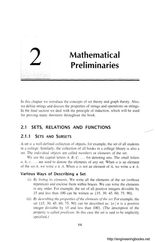
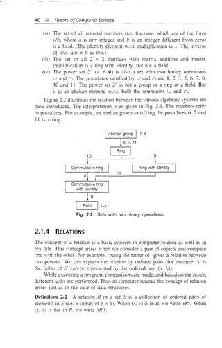
2. MATHEMATICAL PRELIMINARIES
2.1 Sets, Relations and Functions 36
2.1.1 Sets and Subsets 36
2.1.2 Sets with One Binary Operation 37
2.1.3 Sets with Two Binary Operations 39
2.1.4 Relations 40
2.1.5 Closure of Relations 43
2.1.6 Functions 45
2.2 Graphs and Trees 47
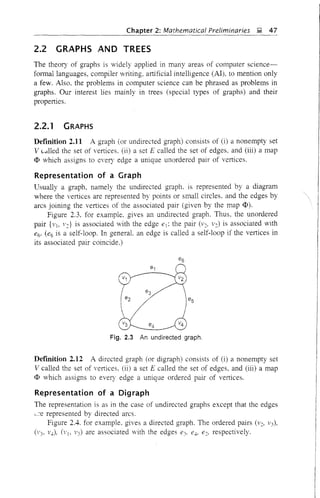
2.2.1 Graphs 47
2.2.2 Trees 49
2.3 Strings and Their Properties 54
2.3.1 Operations on Strings 54
2.3.2 Terminal and Nonterrninal Symbols 56
2.4 Principle of Induction 57
2.4.1 Method of Proof by Induction 57
2.4.2 Modified Method of Induction 58
2.4.3 Simultaneous Induction 60
2.5 Proof by Contradiction 61
2.6 Supplementary Examples 62
Self-Test 66
Exercises 67
36-70
3. THE THEORY OF AUTOMATA 71-106
3.1 Definition of an Automaton 7]
3.2 Description of a Finite Automaton 73
3.3 Transition Systems 74
3.4 Propeliies of Transition Functions 75
3.5 Acceptability of a String by a Finite Automaton 77
3.6 Nondeterministic Finite State Machines 78
3.7 The Equivalence of DFA and NDFA 80
3.8 Mealy and Moore Models 84
3.8.1 Finite Automata with Outputs 84
3.8.2 Procedure for Transforming a Mealy Machine
into a Moore Machine 85
3.8.3 Procedure for Transforming a Moore Machine
into a Mealy Machine 87
3.9 Minimization of Finite Automata 91
3.9.1 Construction of Minimum Automaton 92
3.10 Supplementary Examples 97
Self-Test 103
Exercises ]04
http://engineeringbooks.net](https://image.slidesharecdn.com/automata-150510143406-lva1-app6891/85/Automata-4-320.jpg)


![Symbol
T
F
v
T
F
Ar;;;B
o
AuB
AuE
AxB
Notations
Meaning
Truth value
False value
The logical connective NOT
The logical connective AND
The logical connective OR
The logical connective IF ... THEN
The logical connective If and Only If
Any tautology
Any contradiction
For every
There exists
Equivalence of predicate fonnulas
The element a belongs to the set A.
The set A is a subset of set B
The null set
The union of the sets A and B
The intersection of the sets A and B
The complement of B in A
The complement of A
The power set of A.
The cartesian product of A and B
xi
Section in 'vhich the
srmbol appears first
and is explained
1.1
1.1
1.1
1.1
1.1
1.1
1.1
1.1
1.1
1.4
1.4
1.4
2.1.1
21.1
2.1.1
2.1.1
2.].1
2.1.1
2.1.1
2.1.1
2.1.1
http://engineeringbooks.net](https://image.slidesharecdn.com/automata-150510143406-lva1-app6891/85/Automata-11-320.jpg)
![xii ~ Notations
Symbol Meaning Section in which the
symbol appears first
and is explained
n
UA;
i:::::!
*, 0
xRy
xR'y
i =j modulo n
Cn
R+
R*
R] 0 Rz
f: X -7 Y
f(x)
rxl
L*
Ixl
(Q, L, 0, qo, F)
q:
$
(Q, L, 0. Qo, F)
(Q, L, fl, 0, )" qo)
Irk
(~v, L, P, S)
a=?f3G
*
a=?f3G
a~f3
G
L(G)
,io
The union of the sets AI> Az, ..., An
Binary operations
x is related to y under the relation
x is not related to y under the relation R
i is congruent to j modulo n
The equivalence class containing a
The transitive closure of R
The reflexive-transitive closure of R
The composite of the relations R1 and Rz
Map/function from a set X to a set Y
The image of x under f
The smallest integer;::; x
The set of all strings over the alphabet set L
The empty string
The set of all nonempty strings over L
The lertgthof the string x
A finite automaton
Left endmarker in input tape
Right endmarker in input tape
A transition system
A MealyIMoore machine
Partition corresponding to equivalence of states
Partition corresponding to k-equivalence of states
A grammar
a directly derives f3 in grammar G
a derives f3 in grammar G
a derives f3 in nsteps in grammar G
The language generated by G
The family of type 0 languages
The family of context-sensitive languages
2.1.2
2.1.2, 2.1.3
2.1.4
2.1.4
2.1.4
2.1.4
2.1.5
2.1.5
2.1.5
2.1.6
2.1.6
2.2.2
2.3
2.3
2.3
2.3
3.2
3.2
3.2
3.3
3.8
3.9
3.9
4.1.1
4.1.2
4.1.2
4.1.2
4.1.2
4.3
4.3
The family of context-free languages 4.3
The family of regular languages 4.3
The union of regular expressions R] and Rz 5.1
The concatenationof regular expressions R] and Rz 5.1
The iteration (closure) of R 5.1
http://engineeringbooks.net](https://image.slidesharecdn.com/automata-150510143406-lva1-app6891/85/Automata-12-320.jpg)


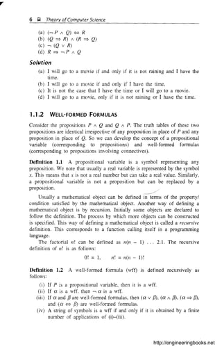


![10 !!!! Theory ofComputer Science
TABLE 1.11 Logical Identities
11 Idempotent laws:
P v P '" P, P ; P '" P
12 Commutative laws:
P v Q '" Q v P, p; Q '" Q 1 P
13 Associative laws:
P v (Q v R) '" (P v Q) v R,
14 Distributive laws:
P 1 (Q 1 R) '" (P ; Q) 1 R
P 1 (P V Q) '" P
by using the distributive law (i.e. 14)
by using Is
by using 19
by using 112
by using the commutative law (i.e. 12)
by using the distributive law (i.e. 14)
by using the DeMorgan's law (i.e. 16)
by using the commutative law (i.e. 12)
,by using 1]2
P v (Q 1 R) '" (P v Q) 1 (P v R), P ; (Q v R) '" (P ; Q) v (P 1 R)
----_._----_._~-~-_ .._--------_ - -_._, ,.__._._ _ - ~ ~ - - -
Is Absorption laws:
P v (P 1 Q) ",p.
Is DeMorgan's laws:
---, (P v Q) '" ---, P 1 ---, Q, ---, (P 1 Q) '" ---, P v ---, Q
17 Double negation:
P '" ---, (-, P)
18 P V ---, P '" T, P 1 ---, P '" F
19 P v T '" T, P 1 T '" P, P v F '" P, P 1 F '" F
~~I__~ Q) 1 (P =} ---, Q) =- ~____ ~ ~~ ~~ ~~_._... .. _
111 Contrapositive:
P=}Q"'---,Q=}---,P
112 P =} Q '" (-, P v Q)
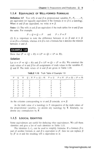
EXAMPLE 1.9
Show that (P 1 Q) V (P 1 --, Q) == P.
Solution
L.H.S. =(P 1 Q) V (P 1 --, Q)
== P 1 (Q V --, Q)
==PIT
== P
= R.H.S.
EXAMPLE 1.10
Show that (P ~ Q) 1 (R ~ Q) == (P v R) ~ Q
Solution
L.H.S. =(P ~ Q) 1 (R ~ Q)
== (--, P v Q) 1 (--, R v Q)
== (Q v --, P) 1 (Q V --, R)
== Q v (--, P 1 --, R)
== Q v (--, (P v R))
== (--, (P v R)) v Q
== (P v R) ~ Q
= R.H.S.
http://engineeringbooks.net](https://image.slidesharecdn.com/automata-150510143406-lva1-app6891/85/Automata-23-320.jpg)

![12 ~ Theory ofComputer Science
== P v P v Q v -, Q v -, R by using 13
== P v Q v -, Q v -, R by using Ii
Thus, P v Q v -, Q v -, R is a disjunctive normal form of the given formula.
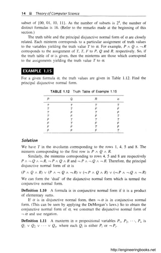
EXAMPLE 1.12
Obtain the disjunctive normal form of
(P ; -, (Q ; R)) v (P =} Q)
Solution
(P ; -, (Q ; R)) v (P =} Q)
== (P ; -, (Q ; R) v (---, P v Q) (step 1 using 1d
== (P ; (-, Q v -, R)) v (---, P v Q) (step 2 using 17)
== (P ; -, Q) v (P ; -, R) v -, P v Q (step 3 using 14 and 13)
Therefore, (P ; -, Q) v (P ; -, R) v -, P v Q is a disjunctive normal form
of the given formula.
For the same formula, we may get different disjunctive normal forms. For
example, (P ; Q ; R) v (P ; Q ; -, R) and P ; Q are disjunctive normal
forms of P ; Q. SO. we introduce one more normal form, called the principal
disjunctive nomwl form or the sum-of-products canonical form in the next
definition. The advantages of constructing the principal disjunctive normal
form are:
(i) For a given formula, its principal disjunctive normal form is unique.
(ii) Two formulas are equivalent if and only if their principal disjunctive
normal forms coincide.
Definition 1.8 A minterm in n propositional variables p], .,', P/1 is
QI ; Q2 ' " ; Q/l' where each Qi is either Pi or -, Pi'
For example. the minterms in PI and P2 are Pi ; P2, -, p] ; P 2,
p] ; -, P'J -, PI ; -, P2, The number of minterms in n variables is 2/1.
Definition 1.9 A formula ex is in principal disjunctive normal form if ex is
a sum of minterms.
1.2.2 CONSTRUCTION TO OBTAIN THE PRINCIPAL
DISJUNCTIVE NORMAL FORM OF A GIVEN FORMULA
Step 1 Obtain a disjunctive normal form.
Step 2 Drop the elementary products which are contradictions (such as
P ; -, P),
Step 3 If Pi and -, Pi are missing in an elementary product ex, replace ex by
(ex; P) v (ex; -,PJ
http://engineeringbooks.net](https://image.slidesharecdn.com/automata-150510143406-lva1-app6891/85/Automata-25-320.jpg)

![Chapter 1: Propositions and Predicates ~ 17
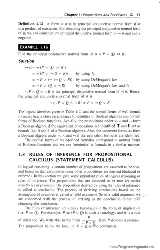
EXAMPLE 1.17
Can we conclude S from the following premises?
(i) P =} Q
(ii) P =} R
(iii) -,( Q / R)
(iv) S j P
Solution
The valid argument for deducing S from the given four premises is given as
a sequence. On the left. the well-formed fOlmulas are given. On the right, we
indicate whether the proposition is a premise (hypothesis) or a conclusion. If
it is a conclusion. we indicate the premises and the rules of inference or logical
identities used for deriving the conclusion.
1. P =} Q Premise (i)
2. P =} R Premise (ii)
3. (P =} Q) / (P => R) Lines 1. 2 and RI2
4. ---, (Q / R) Premise (iii)
5. ---, Q j ---, R Line 4 and DeMorgan's law (h)
6. ---, P v ---, P Lines 3. 5 and destructive dilemma (RI9)
7. ---, P Idempotent law I]
8. S v P Premise (iv)
9. S Lines 7, 8 and disjunctive syllogism Rh
Thus, we can conclude 5 from the given premises.
EXAMPLE 1.18
Derive 5 from the following premises using a valid argument:
(i) P => Q
(ii) Q => ---, R
(iii) P v 5
(iv) R
Solution
1. P =} Q Premise (i)
2. Q => ---, R Premise (ii)
3. P => ---, R Lines 1, 2 and hypothetical syllogism RI7
4. R Premise (iv)
5. ---, (---, R) Line 4 and double negation h
6. ---, P Lines 3. 5 and modus tollens RIs
7. P j 5 Premise (iii)
8. 5 Lines 6, 7 and disjunctive syllogism RI6
Thus, we have derived S from the given premises.
http://engineeringbooks.net](https://image.slidesharecdn.com/automata-150510143406-lva1-app6891/85/Automata-30-320.jpg)


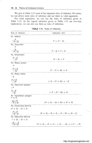
![48 l; Theory ofComputer Science
Fig. 2.4 A directed graph.
DefInitions (i) If (Vi, Vi) is associated with an edge e, then Vi and Vj are called
the end vertices of e; Vi is called a predecessor of Vj which is a successor of Vi'
In Fig. 2.3. 1'~ and 1'3 are the end vertices of e3' In Fig. 2.4, v~ is a
predecessor of 1'3 which is a successor of V~. Also, 1'4 is a predecessor of v~ and
successor of 1'3'
(ii) If G is a digraph, the undirected graph corresponding to G is the
undirected graph obtained by considering the edges and vertices of G, but
ignoring the 'direction' of the edges. For example, the undirected graph
corresponding to the digraph given in Fig. 2.4 is shown in Fig. 2.5.
Fig. 2.5 A graph.
DefInition 2.13 The degree of a vertex in a graph (directed or undirected) is
the number of edges with V as an end vertex. (A self-loop is counted twice while
calculating the degree.) In Fig. 2.3, deg(1']) =2, deg(1'3) =3, deg(1'2) =5. In
Fig. 2.4, deg(1'~) = 3, deg(1'4) = 2.
We now mention the following theorem without proof.
Theorem 2.4 The number of vertices of odd degree in any graph (directed or
undirected) is even.
DefInition 2.14 A path in a graph (undirected or directed) is an alternating
sequence of vertices and edges of the form v]e]1'~e~ ... vn_len_]VI1' beginning
and ending with vertices such that ei has Vi and Vi+] as its end vertices and
no edge or vertex is repeated in the sequence. The path is said to be a path
from 1'1 to VIZ"
For example. 1'je~1'3e3v2 is a path in Fig. 2.3. It is a path from V] to 1'2' In
Fig. 2.4. Vje2V3e3v2 is a path from v] to 1'2' vlej1'2 is also a path from Vj to 1'2'](https://image.slidesharecdn.com/automata-150510143406-lva1-app6891/85/Automata-61-320.jpg)

![Chapter 2: Mathematical Preliminaries J;1 51
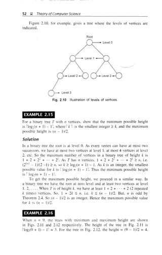
By adopting the following convention, we can simplify Fig. 2.8. The root
is at the top. The directed edges are represented by arrows pointing downwards.
As all the arrows point downwards, the directed edges can be simply
represented by lines sloping downwards, as illustrated in Fig. 2.9.
Fig. 2.9 Representation of an ordered directed tree.
Note: An ordered directed tree is connected (which follows from T2). It has
no circuits (because of T3). Hence an ordered directed tree is a tree (see
Definition 2.17).
As we use only the ordered directed trees in applications to grammars, we
refer to ordered directed trees as simply trees.
Defmition 2.19 A binary tree is a tree in which the degree of the root is 2 and
the remaining vertices are of degree 1 or 3-
Note: In a binary tree any vertex has at most two successors. For example, the
trees given by Figs. 2.11 and 2.12 are binary trees. The tree given by Fig. 2.9
is not a binary tree.
Theorem 2.5 The number of vertices in a binary tree is odd.
Proof Let n be the number of vertices. The root is of degree 2 and the
remaining n - 1 vertices are of odd degree (by Definition 2.19). By
Theorem 2.4, n - 1 is even and hence 11 is odd. I
We now introduce some more terminology regarding trees:
(i) A son of a vertex v is a successor of 1'.
(ii) The father of v is the predecessor of 1'.
(iii) If there is a directed path from v] to 1'2> VI is called an ancestor of V.:,
and V2 is called a descendant of V1' (Convention: v] is an ancestor of
itself and also a descendant of itself.)
(iv) The number of edges in a path is called the length of the path.
(v) The height of a tree is the length of a longest path from the root. For
example, for the tree given by Fig. 2.9, the height is 2. (Actually there
are three longest paths, 1'1 -+ 1'2 -+ V.., 1'1 -+ 1'3 -+ VS, VI -+ V2 -+ V6'
Each is of length 2.)
(vi) A vertex V in a tree is at level k if there is a path of length k from the
root to the vertex V (the maximum possible level in a tree is the height
of the tree).](https://image.slidesharecdn.com/automata-150510143406-lva1-app6891/85/Automata-64-320.jpg)


![Chapter 2: Mathematical Preliminaries ~ 59
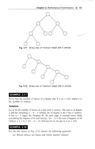
Consider a tree T with (n + 1) vertices as shown in Fig. 2.16. Let e be
an edge connecting the vertices Vi and 1} There is a unique path between Vi
and vi through the edge e. (Property of a tree: There is a unique path between
every pair of vertices in a tree.) Thus, the deletion of e from the graph will
divide the graph into two subtrees. Let nl and n: be the number of vertices
in the subtrees. As 111 ::; 11 and 11: ::; n. by induction hypothesis, the total
number of edges in the subtrees is 11] - 1 + n: - 1. i.e. n - 2. So, the number
of edges in T is n - 2 + 1 =11 - 1 (by including the deleted edge e). By
induction. the result is true for all trees.
e
Fig. 2.16 Tree T with (n + 1) vertices.
EXAMPLE 2.23
Two definitions of palindromes are given below. Prove by induction that the
two definitions are equivalent.
Definition 1 A palindrome is a string that reads the same forward and
backward.
Definition 2 (i) A is a palindrome.
(ii) If a is any symboL the string a is a palindrome.
(iii) If a is any symbol and x is a palindrome. then axa is a palindrome.
(iv) Nothing is a palindrome unless it follows from (i)-(iii).
Solution
Let x be a string which satisfies the Definition L i.e. x reads the same forward
and backward. By induction on the length of x we prove that x satisfies
the Definition 2.
If Ix I ::; 1. then x =a or A. Since x is a palindrome by Definition L i
and a are also palindromes (hence (i) and (ii», i.e. there is basis for induction.
If !x I > 1. then x =mva, where w. by Definition 1. is a palindrome: hence the
rule (iii). Thus. if x satisfies the Definition L then it satisfies the Definition 2.
Let x be a string which is constructed using the Definition 2. We
show by induction on ix I that it satisfies the Definition 1. There is basis
for induction by rule (ii). Assume the result for all strings with length < n.
Let x be a string of length n. As x has to be constructed using the
rule (iii). x = aya. where y is a palirrlr'Jme. As y is a palindrome by
Definition 2 and Iy I< 71, it satisfies the Definition 1. So, x = aya also satisfies
the Definition 1.](https://image.slidesharecdn.com/automata-150510143406-lva1-app6891/85/Automata-72-320.jpg)
![60 J;l Theory of Computer Science
EXAMPLE 2.24
Prove the pigeonhole principle.
Proof We prove the theorem by induction on m. If m =1 and 11 > L then
all these 11 items must be placed in a single place. Hence the theorem is true
for III = 1.
Assume the theorem for m. Consider the case of III + 1 places. We prove
the theorem for 11 =In + 2. (If 11 > In + 2. already one of the In + 1 places will
receive at least two objects from m + 2 objects, by what we are going to prove.)
Consider a particular place. say, P.
Three cases arise:
(i) P contains at least two objects.
(ii) P contains one object
(iii) P contains no object.
In case (i). the theorem is proved for n = 111 + 2. Consider case (ii). As P
contains one object, the remaining m places should receive 111 + 1 objects. By
induction hypothesis, at least one place (not the same as P) contains at least two
objects. In case (iii), III + 2 objects are distributed among In places. Once again,
by induction hypothesis, one place (other than P) receives at least two objects.
Hence. in aD the cases, the theorem is true for (m + 1) places. By the principle
of induction. the theorem is true for all Ill.
2.4.3 SIMULTANEOUS INDUCTION
Sometimes we may have a pair of related identities. To prove these, we may
apply two induction proofs simultaneously. Example 2.25 illustrates this
method.
EXAMPLE 2.25
A sequence Fo, F], F2, ... called the sequence of Fibonacci numbers (named
after the Italian mathematician Leonardo Fibonacci) is defined recursively as
follows:
Prove that:
Fo = O.
P" : (2.2)
(2.3)
Proof We prove the two identities (2.2) and (2.3) simultaneously by
simultaneous induction. PI and Q] are F12
+ F0
2
= F1 and F2F 1 + F]Fo = Fc](https://image.slidesharecdn.com/automata-150510143406-lva1-app6891/85/Automata-73-320.jpg)


![Chapter 2: Mathematicai Preiiminaries ~ 65
EXAMPLE 2.33
Prove Property 5 stated in Section 2.2.2.
Solution
We prove the result by induction on n. Obviously, there is basis for induction.
Assume the result for connected graphs with n - 1 vertices. Let T be a
connected graph with II vertices and J1 - 1 edges. By Example 2.32, T has at
least one leaf v (say).
Drop the vertex '.' and the (single) edge incident vith v. The resulting graph
Of is still connected and has 11 - 1 vertices and n 2 edges. By induction
hypothesis. Of is a tree. So 0' has no circuits and hence 0 also has no circuits.
(Addition of the edge incident with v does not create a circuit in G.) Hence G
is a tree. By the principle of induction, the property is true for all n.
EXAMPLE 2.34
A person climbs a staircase by climbing either (i) two steps in a single stride
or (ii) only one step in a single stride. Find a fonnula for Sen), where Sen)
denotes the number of ways of climbing n stairs.
Solution
When there is a single stair. there is only one way of climbing up. Hence
S(l) =1. For climbing two stairs, there are t'iO ways. viz. two steps in a single
stride or two single steps. So 5(2) :::: 2. In reaching n steps, the person can climb
either one step or two steps in his last stride. For these two choices, the number
of 'ways are sen - 1) and Sen - 2).
So,
Sen) :::: Sen - 1) + Sen - 2)
Thus. Sen) = F(n). the nth Fibonacci number (refer to Exercise 2.20.
at the end of this chapter).
EXAMPLE 2.35
How many subsets does the set {I, 2, .... n} have that contain no two
consecutive integers?
Solution
Let Sn denote the number of subsets of (1. 2, ..., n} having the desired
property. If n = 1. S] =I{ 0, {lr = 2. If 11 = 2, then S~ = i{ 0, {l}. {2}! :::: 3.
Consider a set A with n elements. If a subset having the desired property
'ontains n, it cannot contain n - 1. So there are Sn-~ suchmbsets. If it does
not contain n. there are Sn-l such subsets. So S" =Sn-J + Sn-~' As S =2 =F3
and S~ = 3 = Fl,.
the (n + 2)th Fibonacci numbeL](https://image.slidesharecdn.com/automata-150510143406-lva1-app6891/85/Automata-78-320.jpg)
![66 ~ Theory ofComputer Science
EXAMPLE 2.36
If n ~ 1, show that
1·1 r + 2 -2! + ... + n· n! = (n + I)! - 1
Solution
We prove the result by induction on n. If n = L then 1· I! = 1 = (1 + I)! - I.
So there is basis for induction.
Assume the result for n, i.e.
1 . I! + 2·2! + . . . + n· n r = (n + I)! - 1
Then,
I-I! + 2-2! + ". + n·n! + (71 + 1)·(n + I)!
=(n+1)! 1+(n+1)·(n+1)!
= (n + 1)! (l + 11 + 1) - 1 =(n + 2)! - 1
Hence the result is true for 71 + 1 and by the plinciple of induction, the
result is true for all n ~ 1.
EXAMPLE 2.37
Using induction, prove that 21/ < n! for all n ~ 4.
Solution
For 11 =4. 24
< 4!. So there is basis for induction. Assume 21/ < n!.
Then.
2"+1 = 2" - 2 < n! . 2 < (n + l)n! = (n + I)!
By induction, the result is true for a]] n ~ 4.
SELF-TEST
(c) B
Choose the correct answer to Questions 1-10:
1. (A u A) n (B n B) is
(a) A (b) A n B (d) none of these
2. The reflexive-transitive closure of the relation {(1, 2), (2, 3)} is
(a) {(1, 2), (2, 3), (1, 3)}
(b) {(1, 2), (2. 3), (1, 3), (3, I)}
(c) {(l, 1). (2, 2), (3, 3), O. 3), 0, 2), (2, 3)}
(d) {(1, 1). (2, 2), (3, 3). (1, 3)}
3. There exists a function
f: {I. 2, , ... 1O} ~ {2. 3,4.5,6.7,9, 10. 11, 12}](https://image.slidesharecdn.com/automata-150510143406-lva1-app6891/85/Automata-79-320.jpg)

![68 );1 Theory ofComputer Science
(d) A * ( B*
(e) (A - B)*
(f) (B - A)*
2.2 Let S = {a, b} *. For x, ' E S, define x 0 y = xy, i.e. x 0 .y is obtained
by concatenating x and y.
(a) Is 5 closed under a?
(b) Is 0 associative?
(c) Does 5 have the identity element with respect to 0'1
(d) Is 0 conunutative?
2.3 LeI 5 = i where X is any nonempty set. For A, B <;:; X, let
A 0 B =A u B.
(a) Is 0 commutative and associative?
(b) Does 5 have the identity element with respect to 0'1
(c) If A 0 B =A 0 C. does it imply that B = C?
2.4 Test whether the following statements are tme or false. Justify your
answer.
(a) The set of all odd integers is a monoid under multiplication.
(b) The set of all complex numbers is a group under multiplication.
(c) The set of all integers under the operation 0 given by a 0 b =
a + b - ab is a monoid.
(d) 2s under symmenic difference V defined by A VB =(A - B) u
(B - A) is an abelian group.
2.5 Show that the following relations are equivalence relations:
(a) On a set 5. aRb if a =b.
(b) On the set of all lines in the plane, 1]RI: if IJ is parallel to I:.
(c) On N = {O, 1, 2, ...}. mRn if m differs from n by a multiple
of 3.
2.6 Show that the follOving are not equivalence relations:
(a) On a set 5, aRb if a i= b.
(b) On the set of lines in the plane, I]RI: if 11 is perpendicular to 12,
(e) On N = {O, L 2 }. mRn if m divides n.
(d) On 5 = {L 2 , 1O}. aRb if a + b = 10.
2.7 For x, y in {a, b} *, define a relation R by xRy if Ix I =Iy I. Show that
R is an equivalence relation. What are the equivalence classes?
2.8 For x, ' in {a, b}*, define a relation R by xRy if x is a substring of
y (x is a substring of y if y =ZjXZ: for some string Zj, z:). Is R an
equivalence relation?
2.9 Let R = {(L 2). (2. 3). n, 4), (4. 2), (3. 4)} Find R+, R*.
2.10 Find R* for the following relations:
Ca) R = {(l~ 1). (l~ 2)~ (2~ 1)~ (2, 3), (3. 2)}
(b) R = {(l. 1). (2. 3), 0, 4), (3. 2)}](https://image.slidesharecdn.com/automata-150510143406-lva1-app6891/85/Automata-81-320.jpg)
![Chapter 2: Mathematical Preliminaries ~ 69
(c) R = {(L 1), (2, 2), (3, 3), (4, 4)}
(d) R = {(1, 2), (2. 3), (3, 1), (4, 4)}
2.11 If R is an equivalence relation on S, what can you say about R+. R*?
2.12 Letf:{a, b} * ----:> {a, b} *be given by f(x) =ax for every x E {a, b}*.
Show that f is one-to-one but not onto.
2.13 Let g: {a, b}* ----:> {a, b}* be given by g(x) = xT
. Show that g is
one-to-one and onto.
2.14 Give an example of (a) a tree vith six vertices and (b) a binary tree
with seven vertices.
2.15 For the tree T given in Fig. 2.18, ansv,er the following questions:
(a) Is T a binary tree?
(b) Which vertices are the leaves of T?
(c) How many internal vertices are in T?
(d) Vnat is the height of T?
(e) Wnat is the left-to-right ordering of leaves?
(f) Which vertex is the father of 5?
(g) Which vertices are the sons of 3?
Fig. 2.18 The tree for Exercise 2.15.
2.16 In a get-together. show that the number of persons who know an odd
number of persons is even,
[Hi/){: Use a graph.]
2.17 If X is a finite set show that !2X
I = ?!Xj
2.18 Prove the following by the principle of induction:
(a) i k2 = n(n + li2n + 1)
k=l
(b)
11 1
I -k-(k-+-l)
k=l
n
(17 + 1)
(c) 10211
- 1 is divisible by 11 for all II > 1.](https://image.slidesharecdn.com/automata-150510143406-lva1-app6891/85/Automata-82-320.jpg)


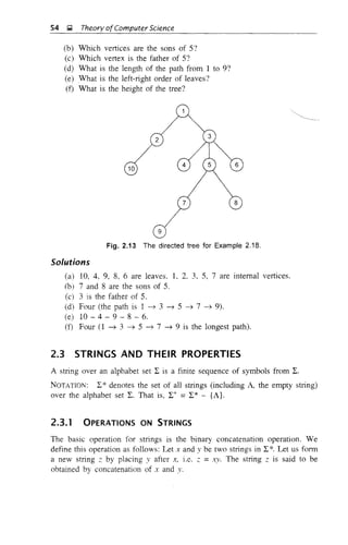
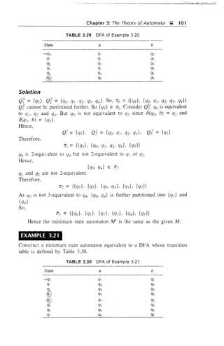
![Chapter 3: The Theory of Automata iii, 77
3.5 ACCEPTABILITY OF A STRING BY A FINITE
AUTOMATON
Definition 3.4 A stling x is accepted by a finite automaton
M = (Q, .L 8, C/o' F)
if D(qo, x) =q for some q E F.
This is basically the acceptability of a string by the final state.
Note: A final state is also called an accepting state.
EXAMPLE 3.5
Consider the finite state machine whose u'unsition function 0 is given by Table 3.1
in the form of a transition table. Here, Q = {CI(), qi. q2> q3}, L = {O, I},
F = {qo}. Give the entire sequence of states for the input string 110001.
TABLE 3.1
State
Transition Function Table for Example 3.5
Input
o
Solution
(--:
-7 ~/
q,
q2
q3
Hence.
l l
8{qo, 110101) = D(C/I.IOIOI)
I
..v
= 0(% 0101)
l
=D(q~, 101)
l
= 8(q3,Ol)
l
=D(q], 1)
= 8(qo, ..1)
J 1 a 1 a j
qo ~ qj ~ qo ~ q~ ~ q3 ~ qj ~ qo
The symbol l indicates that the current input symbol is being processed by the
machine.](https://image.slidesharecdn.com/automata-150510143406-lva1-app6891/85/Automata-90-320.jpg)

![80 9 Theory of Computer Science
-------------------
3.7 THE EQUIVALENCE OF DFA AND NDFA
We naturally try to find the relation between DFA and NDFA. Intuitively we
now feel that:
(i) A DFA can simulate the behaviour of NDFA by increasing the number
of states. (In other words. a DFA (Q, L, 8, qQ, F) can be viewed as an
NDFA (Q, L, 8', qQ, F) by defining 8'(q, a) = {8(q, a)}.)
Oi) Any NDFA is a more general machine without being more powelfuL
We now give a theorem on equivalence of DFA and NDFA.
Theorem 3.1 For every NDFA, there exists a DFA which simulates the
behaviour of NDFA. Alternatively, if L is the set accepted by NDFA, then there
exists a DFA which also accepts L.
Proof Let M = (Q, L, 8, qQ, F) be an NDFA accepting L. We construct a DFA
M' as:
M' =(Q', L, 8, (/o, F')
where
(i) Q' =2Q
(any state in Q' is denoted by [qio q2, .... q;], where qio q2,
.... qj E Q):
(ii) q'0 = [clo]; and
(iii) r is the set of all subsets of Q containing an element of F.
Before defining 8'. let us look at the construction of Q', q'o and r. M is
initially at qo. But on application of an input symbol, say a, M can reach any
of the states 8(qo, a). To describe M, just after the application of the input
symbol a. we require all the possible states that M can reach after the
application of a. So, lvI' has to remember all these possible states at any instant
of time. Hence the states of M' are defined as subsets of Q. As M starts with
the initial state qo, q'o is defined as [qo]. A string w belongs to T(M) if a final
state is one of the possible states that M reaches on processing w. So, a final
state in M' (i.e. an element of F') is any subset of Q containing some final
state of M.
Now we can define 8':
(iv) 8'([qb q2. .... qi], a) = 8(q[, a) u 8(q2, a) u '" U 8(qi' a).
Equivalently.
if and only if
8({ql' ..., q;}, a) = {PI, P2• ..., Pi}'
Before proving L = T(M'), we prove an auxiliary result
8'(q'o, x) = [qj, .. '. q;],
if and only if 8(qo, x) = {qj, "" q;} for all x in P.
We prove by induction on Ix I. the 'if part. i.e.
8'(q'o. x) = [qJ' q2. , ... q;]
if 8(qo. x) = {qJ..... q;}.
(3.4)
(3.5)](https://image.slidesharecdn.com/automata-150510143406-lva1-app6891/85/Automata-93-320.jpg)
![Chapter 3: The Theory of Automata );;I, 81
When Ixl = O. o(qo, A) = {qoL and by definition of o~ [/(q6. A) =
qa =[qol So. (3.5) is true for x with Ixi ::: O. Thus there is basis for induction.
Assume that (3.5) is true for all strings y with Iy I S; m. Let x be a
string of length In + 1. We can write x as va, where 'y' = 111 and a E L. Let
o(qo, 1') = {p, ..., Pi} and o(qo. ya) = {rl' r2' .... rd· As Iyi S; In, by
Induction hypothesis we have
O'(qo· y) = [PI, .... p;] (3.6)
Also.
{rl' r~ .... r;} = O(qo, ya) = O(o(qo, Y). a) ::: O({PI, .... Pj}, a)
By definition of o~
(3.7)
Hence.
O'(q(;. yay = o/(o/(q'o. y), a) = O'([PI . ..., Pi], a) by (3.6)
::: [rl' .... rd by (3.7)
Thus we have proved (3.5) for x = .va.
By induction. (3.5) is true for all strings x. The other part (i.e. the 'only if'
part), can be proved similarly, and so (3.4) is established.
Now. x E T(M) if and only if O(q. x) contains a state of F. By (3.4).
8(qo, x) contains a state of F if and only if 8'(qo, x) is in F'. Hence. x E T(M)
if and only if x E T(Af'). This proves that DFA M' accepts L. I
Vote: In the construction of a deterministic finite automaton M1 equivalent to
a given nondetelministic automaton M, the only difficult part is the construction
of 8/ for M j • By definition.
k
8'([q1 ... qd, a) = U 8(q;, a)
l=l
So we have to apply 8 to (q;. a) for each i = 1. 2..... k and take their
union to get o'([q] .. , qd. a).
When 8 for /1'1 is given in telms of a state table. the construction is simpler.
8(q;, a) is given by the row corresponding to q; and the column corresponding
to a. To construct 8'([ql ... qk]. a), consider the states appearing in the rows
corresponding to qj , ql;o and the column corresponding to a. These states
constitute 8'([q] qd. a).
Note: We write 8' as 8 itself when there is no ambiguity. We also mark the
initial state with ~ and the final state with a circle in the state table.
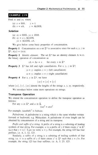
EXAMPLE 3.6
Construct a deterministic automaton equivalent to
M ::: ({qo. qd· {O. l}. 8, qo, {qoD
where 8 is defined by its state table (see Table 3.2).](https://image.slidesharecdn.com/automata-150510143406-lva1-app6891/85/Automata-94-320.jpg)
![82 g Theory ofComputer Science
TABLE 3.2 State Table for Example 3,6
State/L o
~@ qo q,
__--'qC-'-' q--'i qo, ql
Solution
For the deterministic automaton MI.
(i) the states are subsets of {qo. Ql}, i.e. 0. [qo], [c/o' q;], [q;];
(ii) [qoJ is the initial state;
(iii) [qo] and [qo, q;] are the final states as these are the only states
containing qo; and
(iv) 8 is defined by the state table given by Table 3.3.
TABLE 3.3 State Table of M, for Example 3,6
State/'L
o
[qo]
[q,]
[qo, q,]
o
o
[qo]
[q,]
[qo, q,]
o
[q,]
[qo, q,]
[qo, q,]
The states qo and ql appear in the rows corresponding to qo and qj and the
column corresponding to O. So. 8([qo. qt], 0) =[qo. qd·
When M has 11 states. the corresponding finite automaton has 2" states.
However. we need not construct 8 for all these 2" states, but only for those
states that are reachable from [Qo]. This is because our interest is only in
constructing M 1 accepting T(M). So, we start the construction of 8 for [qo]. We
continue by considering only the states appearing earlier under the input
columns and constructing 8 for such states. We halt when no more new states
appear under the input columns.
EXAMPLE 3.7
Find a detefIIljnistic acceptor equivalent to
M = ({qo. qIo q:J. {a. hI. 8. qo. {q2})
where 8 is as given by Table 3.4.
TABLE 3.4 State Table for Example 3.7
State/'L a b
~qo qo. q, q2
q, qo q,
@ qo. q,](https://image.slidesharecdn.com/automata-150510143406-lva1-app6891/85/Automata-95-320.jpg)
![Chapter 3: The Theory of Automata ~ 83
Solution
The detenninisticautomaton M 1 equivalent to M is defined as follows:
M) = (2Q, {a, b}, 8. [q01 F')
where
F ={[cd· [qo, Q2J, [Ql' q2], [qo· % q2]}
We start the construction by considering [Qo] first. We get [q2] and [qo. q:]. Then
we construct 8 for [q2] and [qo. q1]. [q), q2J is a new state appearing under the
input columns. After constructing 8 for [ql' q2], we do not get any new states
and so we terminate the construction of 8. The state table is given by Table 3.5.
TABLE 3.5 State Table of M, for Example 3.7
EXAMPLE 3.8
State/I
[001
[02]
[00, 0']
[a,. 02]
a
[00. 01]
o
[00. a,]
[00]
b
[02]
[00, a,]
[a" 02]
[00, 01]
Construct a deterministic finite automaton equivalent to
M =({qCh qj, 12, q:}, {a, I}), 8. qo, {q3})
where /5 is given by Table 3.6.
TABLE 3.6 State Table for Example 3.8
State/I a b
---'>00 00. a' 00
a, 02 a,
02 03 03
.'C0 02'.:.::.)
Solution
Let Q == {qo, q1' q:, q:,}. Then the deterministic automaton M1 equivalent to
M is given by
MI = (2
Q
• {a. b}. 8, [qo], F)
where F consists of:
[q3]. [qo· q3]. [q1- q3j· [q2' q3]. [qo. qj. Q3], [qo. q2' q3]. [Q]o Q2' Q3]
and
[Qo· Q!. q2. q3]
and where 15 is defined by the state table given by Table 3.7.](https://image.slidesharecdn.com/automata-150510143406-lva1-app6891/85/Automata-96-320.jpg)
![84 !;' Theory ofcomputer Science
TABLE 3.7 State Table of Mi for Example 3.8
State/I a
-_..._--_._------
b
[qo, Cli]
[qc. q1 q2]
[qJ Clil [qol
[qo q,. q2l [qo. q,]
[qQ. q-,. Q2. q3] [qo. q,. q3]
[qo. qi. q3] [qo. q1 Cl2] [qo. Q,. q2]
[qc•. qi. q2. q3] [qc. q, Cl2 q3] [qo. qi. q2.{f31
- - - - - - - - - - - - - - - - - - - - - - - - - - - - - - ' - - -
3.8 MEALY AND MOORE MODELS
3.8.1 FINITE AUTOMATA WITH OUTPUTS
The finite automata vhich we considered in the earlier sections have binary
output i.e. either they accept the string or they do not accept the string. This
acceptability vas decided on the basis of reachahility of the final state by the
initial state. Now. we remove this restriction and consider the mode1 where the
outputs can be chosen from some other alphabet. The value of the output
function Z(t) in the most general case is a function of the present state q(t) and
the present input xU), i.e.
Z(n :::;
where Ie is called the output function. This generalized model is usua!Jy called
the !'v!ca!l' machine. If the output function Z(t) depends only on the present state
and is independent of the cunent input. the output function may be written as
Z(t) :::;
This restricted model is called the j'vJoore machine. It is more convenient to use
Moore machine in automata theory. We now give the most general definitIons
of these machines.
Definition 3.8 A Moore machine is a six-tuple (Q. L, ~. 8, I,. (]ol. where
(il Q is a finite set of states:
I is the input alphabet:
(iii) ~ is the output alphabet:
8 is the transition function I x Q into Q:
I, is the output function mapping Q into ~; and
(]o is the initial state.
Definition 3.9 /'I. Ivlealy machine is a six-tuple (Q, I, ~, 8. )e, qo). "vhere
all the symbols except Ie have the same meaning as in the Moore machine. A.
is the output function mapping I x Q into ,1,
For example. Table 3.8 desclibes a Moore machme. The initial state iJo is
marked with an arrow. The table defines 8 ane! A...](https://image.slidesharecdn.com/automata-150510143406-lva1-app6891/85/Automata-97-320.jpg)

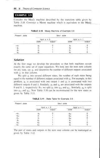


![90 ~ Theory ofComputer Science
1/Z2
Fig. 3.10 Mealy machine of Example 3.12.
Solution
Let us convert the transition diagram into the transition Table 3.19. For the
given problem: qJ is not associated with any output; q2 is associated with two
different outputs Zj and 22; (]3 is associated with two different outputs 21 and
22, Thus we must split q2 into q21 and (]22 with outputs 2 1 and Z2, respectively
and q3 into (]31 and q32 with outputs 2 1 and 22, respectively. Table 3.19 may be
reconstructed as Table 3.20.
TABLE 3.19 Transition Table for Example 3.12
Present state Next state
a = 0 a =
state output state output
q2 Z, q3 Z,
q2 Z2 q3 Z-I
q2 Z, q3 Z2
TABLE 3.20 Transition Table of Moore Machine for Example 3.12
Present state
--,>q,
q21
q22
q31
q32
a =0
Next state
a =1
Output
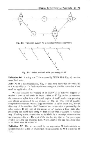
Figure 3.11 gives the transition diagram of the required Moore machine.](https://image.slidesharecdn.com/automata-150510143406-lva1-app6891/85/Automata-103-320.jpg)
![Chapter 3: The Theory of Automata ~ 91
o
Fig. 3.11 Moore machine of Example 3.12.
3.9 MINIMIZATION OF FINITE AUTOMATA
In this section we construct an automaton with the minimum number of states
equivalent to a given automaton M.
As our interest lies only in strings accepted by i!I, what really matters is
whether a state is a final state or not. We define some relations in Q.
DefInition 3.10 Two states ql and q: are equivalent (denoted by qj == q:) if
both o(qj. x) and O(q:. x) are final states. or both of them are nonfinal states
for all x E 2:*.
As it is difficult to construct O(qj, x) and O(q:, x) for all x E 2:* (there
are an infinite number of stlings in 2:*). we give one more definition.
Definition 3.11 Two states qj and q: are k-equivalem (k ;::: 0) if both
O(qj, x) and O(q:. ;r) are final states or both nonfinal states for all strings x
of length k or less. In particular, any two final states are O-equivalent and any
tVO nonfinal states are also O-equivalent.
We mention some of the properties of these relations.
Property 1 The relations we have defined. i.e. equivalence and k-equivalence,
are equivalence relations. i.e. they are reflexive, symmetric and transitive.
Property 2 By Theorem 2.1. these induce partitions of Q. These partitions
can be denoted by Jr and Jrl' respectively. The elements of Jrl are k-equivalence
classes.
Property 3 If qj and q: are k-equivalent for all k ;::: O. then they are equivalent.
Property 4 If ql and q: are (k + I)-equivalent. then they are k-equivalent.
Property 5 ir" =Jr,,+] for some 11. (Jr" denotes the set of equivalence classes
under l1-equivalence.)
The following result is the key to the construction of minimum state
automaton.
RESULT Two states qj and q: are (k + I)-equivalent if (i) they are
k-equivalent; (ii) O(q!. a) and O(q:, a) are also k-equivalent for every a E 2:.](https://image.slidesharecdn.com/automata-150510143406-lva1-app6891/85/Automata-104-320.jpg)
![92 ~ Theory ofComputer Science
Proof We prove the result by contradiction. Suppose qj and q2 are not
(k + I)-equivalent. Then there exists a string W =aWl of length k + 1 such that
8(ql. aWj) is a final state and 8(q'b aWl) is not a final state (or vice versa; the
proof is similar). So 8(8(qb a}. wI) is a final state and 8(8(q:, a), WI) is not
a final state. As WI is a string of length k, 8(q), a) and 8(q:, a) are not
k-equivalent. This is a contradiction. and hence the result is proved. I
Using the previous result we can construct the (k + I)-equivalence classes
once the k-equivalence classes are known.
3.9.1 CONSTRUCTION OF MINIMUM AUTOMATON
Step 1 (Construction of no)· By definition of O-equivalence, no ={Q?, Qf }
where Q? is the set of all final states and Qf =Q - Q?
Step 2 (Construction of lrk+i from lr;:). Let Q/' be any subset in lrk' If q) and
q2 are in Q/'. they are (k + I)-equivalent provided 8(% a) and 8(q']) a) are
k-equivalent. Find out whether 8(qj, a) and 8(q2' a) are in the same equivalence
class in ~k for every a E L. If so. q) and q: are (k + I)-equivalent. In this way,
Q/' is further divided into (k + I)-equivalence classes. Repeat this for every Q/'
in lrk to get all the elements of lrk+)'
Step 3 Construct lr" for 11 = 1. 2, .... until lr" = lrn+!·
Step 4 (Construction of minimum automaton). For the required minimum
state automaton. the states are the equivalence classes obtained in step 3. i.e. the
elements of !rl!' The state table is obtained by replacing a state q by the
conesponding equivalence class [q].
Remark In the above construction, the crucial part is the construction of
equivalence classes; for. after getting the equivalence classes, the table for
minimum automaton is obtained by replacing states by the conesponding
equivalence classes. The number of equivalence classes is less than or equal to
IQ I· Consider an equivalence class [qd = {qj, q:, ..., qd· If qj is reached
while processing WIW: E T(M) with 8(qo, Wj) = qb then 8(Ql. w:) E F. So,
8(q;, w:) E F for i =2...., k. Thus we see that qj. i =2, .. " k is reached on
processing some IV E T(M) iff qj is reached on processing w, i.e. ql of [qd can
play the role of q:. ..., qk' The above argument explains why we replace a state
by the conesponding equivalence class.
Note: The construction of no, lrj, lr:, etc. is easy when the transition table
is given. Jl1J = {QF. Q:o}. where Q? =F and Q:o =Q - F. The subsets in
lrl are obtained by further partitioning the subsets of no· If qj, q: E Q?,
consider the states in each a-column. where a E l: conesponding to qj and q2'
If they are in the same subset of 71';), q) and q: are I-equivalent. If the states
under some a-column are in different subsets of 7i'Q. then ql and q: are not
I-equivalent. In generaL (k + 1)-equivalent states are obtained by applying the
above method for ql and q: in rj/'.](https://image.slidesharecdn.com/automata-150510143406-lva1-app6891/85/Automata-105-320.jpg)

![94 );2 Theory ofComputer Science
The {cd in 7ru cannot be further partitioned. SO, Q = {q::}. Consider qo and
qj E Qt The entries under the O-column corresponding to qo and qj are q]
and qr,: they lie in Q!/ The entries under the I-column are qs and q::. q:: E
Qp and qs E Q::o. Therefore. qo and q are not i-equivalent. Similarly, qo is
not i-equivalent to q3' qs and q7'
Now, consider qo and q4' The entries under the O-column are qj and q7'
Both are in Q::o. The entries under the I-column are qs, qs· So q4 and qo are
I-equivalent. Similarly, qo is I-equivalent to q6' {qo. q4, q6} is a subset in n.
SO, Q':: ={qo, q4' q(,}.
Repeat the construction by considering qj and anyone of the states
q3, qs· Q7' Now, qj is not I-equivalent to qj or qs but I-equivalent to q7' Hence,
Q'3 ={qj, q7}' The elements left over in Q::o are q3 and qs. By considering the
entries under the O-column and the I-column, we see that q3 and q) are
l-equivalent. So Q/4 = {qj, qs}' Therefore,
ITj = {{q:;}. {qo· q4' q6}. {qj. q7}, {q3. qs}}
The {q::} is also in n:: as it cannot be further partitioned. Now, the entries
under the O-column corresponding to qo and q4 are qj and q7' and these lie
in the same equivalence class in nj. The entries under the I-column are qs,
qs. So qo and q4 are 2-eqnivalent. But qo and q6 are not 2-equivalent. Hence.
{qo. Cf4, qd is partitioned into {qo, qd and {qd· qj and q7 are 2-equivalent.
q3 and qs are also 2-equivalent. Thus. n:: = {{q::L {qo, q4}, {Q6}, {Qj, Q7L
{qj, qs}}. qo and q4 are 3-equivalent. The qj and Q7 are 3-equivalent. Also.
q3 and qs are 3-equivalent. Therefore.
nj = {{qJ, {qo, q4}, {q6}, {qj, q7L {Q3, qs}}
As n: = nj. n2 gives us the equivalence classes, the minimum state automaton
is
M' =(Q" {O. I}. 8" qo, Fj
where
Q' = {[q2J. [qo, q4J, [q6]. [qt- Q7], [Q3' Qs]}
qo = [qo, Q4]' F = [cd
and 8/ is defined by Table 3.22.
TABLE 3.22 Transition Table of Minimum State
Automaton for Example 3.13
State/I. 0
[qo, q4] [0', OJ] [03. q5]
[Q1, OJ] [q6] [q2]
[02] [00' 04] [q2]
(Q3· q5] [q2] [06]
[06] [q6] [qo, q4]](https://image.slidesharecdn.com/automata-150510143406-lva1-app6891/85/Automata-107-320.jpg)
![Chapter 3: The Theorv of Automata ~ 95
-----------------"----
Note: The transition diagram for the minimum state automaton is described
by Fig. 3.13. The states qo and q.', are identified and treated as one state.
(SO also are ql, q7 and q3' qs) But the transitions in both the diagrams (i.e.
Figs. 3.12 and 3.13) are the same. If there is an arrow from qi to (jj with label
a. then there is an arrow from [q;J to lq;] with the same label in the
diagram for minimum state automaton. Symbolically, if O(qi' a) = 'ii' then
8'([q;], a) = [q;J.
1
I---~o-_ _A7 [q2]
o
o !'
Fig. 3.13 Minimum state automaton of Example 3,13,
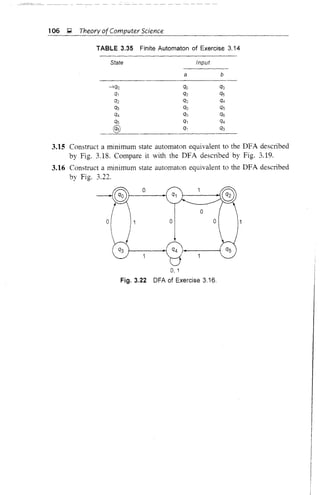
EXAMPLE 3.14
Construct the minimum state automaton equivalent to the transition diagram
given by Fig. 3.14.
b a
-G- b 0- ' ~!'~ I~ b tI I
I I I '
a I
'I :' I' b I r;1 , I ~ ,
~ ~ ~
0- --:~) ~--(i))b
b
Fig. 3.14 Finite automaton of Example 3,14,
Solution
We construct the transition table as given by Table ,3.23.](https://image.slidesharecdn.com/automata-150510143406-lva1-app6891/85/Automata-108-320.jpg)

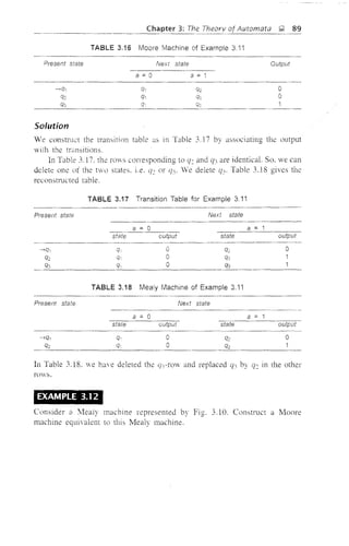
![Chapter 3: The Theorv of Automata i;l 97
where
Q' = {[cI3], [qo, Q6], [ql' qs], [q:> q4], [q7]}
q'o = [qo, qd, r = [q3]
and 8' is defined by Table 3.24.
TABLE 3.24 Transition Table of Minimum State
Automaton for Example 3,14
State/I. a b
[qQ, q6] [q1' q5] [qQ, q6]
[q1' q5] [qQ, q6] [q2, q4]
[q2, q4] [q31 [q1, q5]
[q3] [q3] [qQ' q6]
[q7] [qQ, q6] [q3]
Note: The transition diagram for lVI' is given by Fig. 3.15.
b
b
Fig. 3.15 Minimum state automaton of Example 3,14,
3.10 SUPPLEMENTARY EXAMPLES
EXAMPLE' 3.15
Construct a DFA equivalent to the li'DFA M whose transition diagram is given
by Fig. 3.16.
a, b
a, 0 q1
I
b
I
~ j'
q2 a
Fig. 3.16 NDFA of Example 3,15](https://image.slidesharecdn.com/automata-150510143406-lva1-app6891/85/Automata-110-320.jpg)
![98 Q Theory ofComputer Science
Solution
The transition table of M is given by Table 3.25.
TABLE 3.25 Transition Table for Example 3.15
State a b
For the equivalent DFA:
(i) The states are subsets of Q ={qo, CJl, CJ2, Q3, Q4}'
(ii) [qo] is the initial state.
(iii) The subsets of Q containing Q3 or Q4 are the final states.
(iv) 8 is defined by Table 3.26. We start from [qoJ and construct 8, only
for those states reachable from [qoJ (as in Example 3.8).
TABLE 3.26 Transition Table of DFA for
Example 3.15
State
[qQ]
[qQ. qzl
[qQ. q4]
a
[qQ]
[qo. q4]
[qo]
b
[qQ, q2]
[qQ- qzJ
[qQ. q2]
EXAMPLE 3.16
Construct a DFA equivalent to an NDFA whose transition table is defined by
Table 3.27.
TABLE 3.27 Transition Table of NDFA for
Example 3.16
State a b
Solution
Let i'v! be the DFA defined by
M = C{'!"·()I·'i2· Q3}, {a, b}, 0, [gal F)](https://image.slidesharecdn.com/automata-150510143406-lva1-app6891/85/Automata-111-320.jpg)
![~- -~-~-- ----------~~-
Chapter 3: The Theory ofAutomata ~ 99
where F is the set of all subsets of {qo, qj' Q2' (/3} containing CJJ. <5 is defined
by Table 3.28.
TABLE 3.28 Transition Table of DFA for
Example 3.16
State
[qo]
[q,. q3]
[qd
[q3]
[Q2. q3]
[q2]
o
a
[q1. q3]
[q,]
[QJ
o
[q3]
[q3]
o
b
[Q2. q3]
[q3]
[Q3]
o
EXAMPLE 3.17
Construct a DFA accepting all strings Hover {O, I} such that the numher of
l' s in H' is 3 mod 4.
Solution
Let ;J be the required NDFA. As the condition on strings of T(M) does not
at all involve 0. we can assume that ;J does not change state on input O. If 1
appears in H' (4k + 3) times. M can come back to the initial state. after reading
4 l's and to a final state after reading 31's.
The required DFA is given by Fig. 3.17.
Fig. 3.17 DFA of Example 3.17.
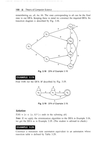
EXAMPLE 3.18
Construct a DFA accepting all strings over {a. h} ending in abo
Solution
We require t/O transitions for accepting the string abo If the symbol b is
processed after an or ba. then also we end in abo So we can have states for](https://image.slidesharecdn.com/automata-150510143406-lva1-app6891/85/Automata-112-320.jpg)
![102 ~ Theory orComputer Science
Solution
Q? = {q3' (r~}, Q~ = {qo. ql' q2' q), q6' q7}
1fo = {{Q3, q4}, {qo. qj, Q2, qs, q6' q7}}
q3 IS I-equivalent to q4' So, {q3' q4} E 1f1'
qo is not I-equivalent to ql, q2, Cis but q() is I-equivalent to Q6'
Hence {q(). qd E 1f1. ql is I-equivalent to q2 but not I-equivalent to
qs, q6 or q7' So, {Ql' C!2} E 1f1'
qs is not I-equivalent to q6 but to q7' So, {Cis, q7} E 1fJ
Hence,
Jrl = {{q3' CJ4}' {q(), qe,}, {ql' q2}, {q5' (j7}}
q3 is 2-equivalent to q4' So, {q3, q4} E Jr2'
qo is not 2-equivalent to Q6' So. {qo}· {CJ6} E Jr2'
qJ is 2-equivalent to q2' So. {qj, Q:J E Jr~.
qs is 2-equivalent to q7. So, {qs, q7} E Jr2'
Hence.
q3 is 3-equivalent to q4; qj is 3-equivalent to q2 and Cis is 3-equivalent to qi'
Hence.
As Jr3 = Jr2' the minimum state automaton is
where 8/ is defined by Table 3.31.
TABLE 3.31 Transition Table of OFA for
Example 3.21
Slate a b
[qo] [q1. q2] [q1' q2]
[q1 q2] [q3, q4] [Q3, q4]
[q3, q4] [qs, q7] [qs]
[qs. q7] [q3. q4] [qs]
[qs] [qs] [qs]](https://image.slidesharecdn.com/automata-150510143406-lva1-app6891/85/Automata-115-320.jpg)
![Chapter 3: The Theory ofAutomata g 103
SELF-TEST
Study the automaton given in Fig. 3.20 and choose the correct answers
to Questions 1-5:
-iGJpo
1,/-
/
oc£5 1 .8Jo
Fig. 3.20 Automaton for Questions 1-5
1. M is a
(a) nondeterministic automaton
(b) deterministic automaton accepting {O. I} *'
(c) deterministic automaton accepting all strings over {O, I} having
3m O's and 3n ]'s, m. 11 2 1
(d) detelministic automaton
2. M accepts
(a) 01110 (b) 10001 (e) 01010 (d) 11111
3. T(M) is equal to
(a) {03111 1311
1m. 11 2 O}
(b) {O'm 1311
Im. n 2:: I}
(e) {1 IH' has III as a substring}
(d) {H IH' has 31i l·s. 11 2 I}
4. If q2 is also made a final state. then At accepts
(a) 01110 and 01100
(b) 10001 and 10000
(c) 0110 but not 0111101
(d) 0311
• 11 2:: 1 but not 1311
• 11 2:: 1
5. If q: is also made a final state, then T(M) is equal to
(a) {03111
13
/1 I In, 11 2 O} u {02111
1" I m, 11 2 O}
(b) {03m 13n
I m. Ii 2 I} u {O:'" I" I m. 11 2:: I}
(c) {H' IH' has III as a substring or 11 as a substring}
(d) {w I the number of l's in ]V is divisible by 2 or 3}
Study the automaton given in Fig. 3.21 and state whether the Statements
6-15 are true or false:
0.1 0,1
@1---O-'~0
Fig. 3.21 Automaton for Statements 6-15](https://image.slidesharecdn.com/automata-150510143406-lva1-app6891/85/Automata-116-320.jpg)


![<adverb> ,
108 ~ Theory of Compurer Science
past tense, and 'quickly' by 'slowly', l.e. by any adverb. we get other
grammatically correct sentences. So the structure of 'Ram ate quickly' can be
given as (noun) (verb) (adverb). For (noun) we can substitute 'Ram'. 'Sam',
'Tom'. 'Gita', etc. . Similarly. we can substirure "ate'. 'walked', 'ran', etc. for
(verb). and 'quickly". 'slowly' for (adverb). Similarly, the structure of 'Sam ran'
can be given in the form (noun)
We have to note that (noun) (vdb) is not a sentence but only the
description of a particular type of sentence. If we replace (noun), (verb) and
(adverb) by suitable vords, we get actual grammatically correct sentences. Let
us call (noun), (adverb) as variables. Words like 'Ram', 'Sam', 'ate',
'ran'. 'quickly", 'slowly' which form sentences can be caHed terminals. So our
sentences tum out to be strings of terminals. Let S be a variable denoting a
sentence. Now. we can form the following rules to generate two types of
sentences:
S -+ (noun) (verb)
5 --.+ (noun) (verb)
(noun) -+ Sam
(noun) -+ Ram
(noun) -+ Gita
-+ ran
(verb) -+ ate
(verb) -+ walked
(adverb) -+ slowly
(adverb) -+ quickly
(Each arrow represents a rule meaning that the word on the right side of the
alTOW can replace the word on the left side of the arrow.) Let us denote the
collection of the mles given above by P.
If our vocabulary is thus restricted to 'Ram', 'Sam', 'Gila', 'ate', 'ran"
'walked', 'quickly' and 'slowly', and our sentences are of the fonn (noun)
(verb) (adverb) and (noun) (verb). we can describe the grammar by a 4-tuple
(V" I, P, S), where
li = {(noun). (verb). (adverb)!
I = {Ram, Sam, Gita. ale. ran. walked, quickly, slowly}
P is the collection of rules described above (the rules may be called
productions),
S ]s the special symbol denoting a sentence.
The sentences are obtained by (i) starting with S. (ii) replacing words
using the productions. and (iii) terminating when a string of terminals is
obtained.
Vith this background ve can give the definition of a grmmnar. As
mentioned earlier. this defil1ltion is due to Noam Chomsky.](https://image.slidesharecdn.com/automata-150510143406-lva1-app6891/85/Automata-121-320.jpg)
![Chapter 4: Formal Languages J;;;; 109
4.1.1 DEFINITION OF A GRAMMAR
Definition 4.1 A phrase-structure grammar (or simply a grammar) IS
WI, L, P, 5), where
(i) Vv is a finite nonempty set V'hose elements are called variables,
(ii) L is a finite nonempty set 'whose elements are called terrninals,
VI (', L = 0.
(iv) 5 is a special variable (i.e, an element of Ii,J called the start symboL
and
P is a finite set vhose elements are a -7 {3. vhere a and {3 are strings
on u 2:. a has at least one symbol from V The elements of Pare
called productions or production rules or revriting rules.
Note: The set of productions is the kemel of grammars and language
specification. We obsene the following regarding the production rules.
0) Reverse substitution is not permitted. For example, if S -7 AB is a
production, then we can replace S by AB. but we cannot replace AB
by S.
(ii) No inversion operation is permitted. For example. if S -7 AB IS a
production. it is not necessary that AB -7 S is a production.
- - - - - -
EXAMPLE 4.1
G =(VI' L P, S) is a grammar
where
Vy = {(sentence). (noun). (verb). (adverb)}
L = [Ram. Sam. ate, sang. well]
5 =(sentence)
P consists of the follmving productions:
(sentence) -7 (noun) (verb)
(semence) -7 (noun) (verb) (adverb)
(noun) --7 Ram
(noun) ----7 Sam
(verb) -7 ate
( erb) -7 sang
(adverb) ----7 well
NOTATION: (i) If A is any set. then A'" denotes the set of all strings over A.
A+ denotes A. ':' - {;}. where ; is the empty string.
(ii) A, B. C, A1, A2• ... denote the variables.
(ill) a, b, c. ' .. denote the terminals.
(iv) x. y. ;. H •... denote the strings of terminals.
lY, {3, Y. ... denote the elements of (t', u D*.
(vi) ":'{J =< for any symbol X in V u "](https://image.slidesharecdn.com/automata-150510143406-lva1-app6891/85/Automata-122-320.jpg)
![11 0 ~ Theory ofComputer Science
- - - - - - - - - - - - - - - -
4.1.2 DERIVATIONS AND THE LANGUAGE GENERATED
BY A GRAMMAR
Productions are used to derive one stling over /N U L from another string.
We give a formal definition of derivation as follows:
Definition 4.2 If a ~ f3 is a production in a grammar G and y, 8 are any
two strings on U 2:, then we say that ya8 directly derives yf38 in G (we
"!fite this as ya8 ~ yf38). This process is called one-step derivation. In
G
particular. if a ---1 f3 is a production. then a ~ f3.
G
Note: If a is a part of a stling and a ~ f3 is a production. we can replace
a by f3 in that string (without altenng the remaining parts). In this case we
say that the string we started with directly derives the new string.
For example,
G =US}. {O. I}, {S -t 051. S -t Ol}, 5)
has the production 5 ---1 OS1. So, 5 in 04S14
can be replaced by 051. The
resulting string is 04
0511". Thus. we have 04
51"+ ~ 0"OS114
.
G
Note: ~ induces a relation R on IVy U 2:)*. i.e. aRf3 if a ~ [3.
G G
Defmition 4.3 If a and f3 are strings on /v U :E, then we say that a derives
~, '"
f3 if a ~ f3. Here ~ denotes the reflexive-transitive closure of the relation ~
G G G
in (Fy U :E)* (refer to Section 2.1.5).
Note: We can note in particular that a 7 a. Also, if a 7 f3. [X '1'= f3, then
there exist strings [Xl- a2, .. " (tll' where II ;::: 2 such that
(X = (X] ~ a2 ~ a3 . .. ~ all = f3
G G G
When a ~ f3 is in n steps. we write a b f3.
G G
Consider. for example. G = ({5}, {O. I}. {S -t OSl, 5 -t OIl, 5).
*
As S ~ 051 ~ 02S12
::::? 03S13, we have S ~ 03S13. We also have
G G G G
03
513
~ 03513
(as (X ~ a).
G G
Definition 4.4 The language generated by a grammar G (denoted by L(G)) is
defined as {w E :E* IS 7 H}. The elements of L(G) are called sentences.
Stated in another way, L(G) is the set of all terminal strings derived from
the start symbol S.
Definition 4.5 If 5 ,;, ex, then a is called a sentential form. We can note
G
that the elements of L(G) are sentential forms but not vice versa.](https://image.slidesharecdn.com/automata-150510143406-lva1-app6891/85/Automata-123-320.jpg)
![Chapter 4: Formal Languages ~ 111
Definition 4.6 Gi and G: are equivalent if L(GJ =L(G:).
Remarks on Derivation
1. Any derivation involves the application of productions. When the
number of times we apply productions is one, we write a =? {3; when
.,. e
it is more than one, ve vrite CY. ~ f3 (Note: a ~ a).
e G
") The string generated by the most recent application of production is
called the working string.
3. The derivation of a string is complete when the working string cannot
be modified. If the final string does not contain any variable. it is a
sentence in the language. If the final string contains a variable. it is a
sentential form and in this case the production generator gets 'stuck'.
NOTATION: (i) We vrite CY. ~ {3 simply as CY. :b {3 if G is clear from the context.
e
(ji) If A ~ CY. is a production where A E Vv, then it is called an
A-production.
(iii) If A ~ ai' A. ~ a:. .. nA. ~ CY.!/! are A-productions. these
productions are written as A ~ ai i CY.: j ... Iam'
We give several examples of grammars and languages generated by them.
EXAMPLE 4.2
If G = ({5}. {a. I}. {5 ~ 051, s ~ A}. S). find L(G).
Solution
As 5 ~ A is a production. S =? A. So A is in L(G). Also. for all n :::: 1.
G
=? 0"51" =? 0"1"
G G
Therefore.
0"1" E L(G) for n :::: a
(Note that in the above derivation, S ~ 051 is applied at every step except
in the last step. In the last step, we apply 5 ~ A). Hence, {O"I" In:::: O} ~ UG).
To show that L(G) ~ {O''1'' i 17 :::: A}. we start with ].V in L(G). The
derivation of It' starts with 5. If S ~ A is applied first. we get A. In this case
].V =A. Othenvise the first production to be applied is 5 ~ 051. At any stage
if we apply 5 ~ A, we get a terminal string. Also. the terminal string is
obtained only by applying 5 ~ A. Thus the derivation of IV is of the foml
l.e.
5 =? 011
51" =? 0"1"
G G
for some n :::: 1](https://image.slidesharecdn.com/automata-150510143406-lva1-app6891/85/Automata-124-320.jpg)
![112 ~ Theory ofComputer Science
Therefore.
LeG) = {Qlll l1
/n 2: Q}
EXAMPLE 4.3
If G = ({5}, {a}, {5 ----;; 55}, 5), find the language generated by G.
Solution
L(G) = 0. since the only production 5 -> 55 in G has no terminal on the
right-hand side.
EXAMPLE 4.4
Let G =({S. C}, {a, b}, P, 5), where P consists of 5 ----;; aCa. C ----;; aCa Ib.
Find L(G).
Solution
S:=;. aea :=;. aba. So aba E L(G)
5 :=;. aCa (by application of 5 ----;; aCa)
b d'Cd' (by application of C ----;; aCa (n - 1) times)
:=;. d'bafl
(by application of C ----;; b)
Hence. a"ba" E LeG), where n :2: 1. Therefore.
{d'ba"ln 2: I} s:: L(G)
As the only S-production is 5 ----;; aCa, this is the first production we have
to apply in the derivation of any terminal string. If we apply C ----;; b. we get aba.
Otherwise we have to apply only C ----;; aCa. either once or several times. So
we get d'Ca" with a single variable C. To get a terminal string we have to
replace C by b. by applying C ----;; b. So any delivation is of the fonn
S b a"bun
with n 2: 1
Therefore.
L(G) s:: {a"bail In 2: ]}
Thus.
L(G) = {(/ball
iJl 2: I}
EXERCISE Construct a grammar G so that UG) = {a"bc/1I
1 n. m 2: l}.
Remark By applying the com'ention regarding the notation of variables.
terminals and the start symbol. it vill be clear from the context whether a
symbol denotes a variable or terminal. We can specify a grammar by its
productions alone.](https://image.slidesharecdn.com/automata-150510143406-lva1-app6891/85/Automata-125-320.jpg)
![Chapter 4: Formal Languages ~ 113
EXAMPLE 4.5
If Gis S ~ as iItS [ a[h, find L(G).
Solution
We shov that U C) = {a. b} 7. As V·le have only two terminals a, h,
UG) :;;;;; {a. b} *. All productions are S-productions. and so A can be in L(G)
on1 when S ~ A is a production in the grammar G. Thus.
UG) :;;;;; {a. h} ':' - {A} = {a, b} +
To show {Cl, br :;;;;; ICG). consider any string al a: ... ali' where each ai
is either a or h. The first production in the delivation of ClI{l2 ... all is S ~
as or 5 ~ bS according as a] = a or (lj = b. The subsequent productions are
obtained in a similar way. The last production is S ~ a or S ~ b according
as = a or a" = b. So aja2 ... ali E UG). Thus. we have L(G) = {a, h]+.
EX~RCISE If G is S ~ as [a, then show that L(G) = {a} +
Some of the following examples illustrate the method of constructing a
grammar G generating a gi ven subset of stlings over E. The difficult P<hrt is the
construction of productions. Ve try to define the given set by recursion and then
declop productions generating the strings in the given subset of E*.
EXAMPLE 4.6
Let L be the set of all pahndromes over {a. h}. Construct a grammar G
generating L.
Solution
S=>bS => (I,
For constructing a grammar G generating the set of all palindromes. ve use
the recursive definition (given in Section 2.4) to observe the following:
ii) A is a palindrome.
Iii) a. b are palindromes.
(Jii) If x is a palindrome axo. then bxb are palindromes.
So e define P as the set consisting of:
S ~.
S ~ (f and S ~ b
Oii) S ~ aSa and S ~ hSb
Let G =({5} {a. b}, P. S). Then
5 => A,
The. fore.
A. a. h E L(G)
If x is a palindrome of even length, then x =a1a2 .. " ([III {[ill .•• a!, where
"'3" ron ' 's el"tJ'e~ '1 (), lJ Tlf1e11 S =>':' " - (,1"1 a 'I b' app'''l'TIa....... ~ L Ui L _d 1 L. ~ • i . d U2 . .. .'1! (Ii; !1i-l ... l-1 "..: <:: _ If b
S --" aSa or S ~ bSb. Thus. x E L(G).](https://image.slidesharecdn.com/automata-150510143406-lva1-app6891/85/Automata-126-320.jpg)

![Chapter 4: Formal Languages ~ 115
EXAMPLE 4.9
Find a grammar generating {a'b"e"! 11 ~ L j ~ O}.
Solution
Let G = ({5, A}, {a. b, e}, P, 5). where P consists of 5 ~ as, 5 ~ A.
A ~ bAe ! be. As in the previous example, we can prove that G is the required
grammar.
EXAMPLE 4.10
Let G =({5. Ad. {O. L 2}. p. 5), where P consists of 5 ~ 05A[2. 5 ~ 012,
2A1 ~ A]2. lA] ~ 11. Show that
L(G) = {0"1"2" I 11 ~ I}
Solution
As 5 ~ 012 is a production, we have 5 ::::} 012, i.e. 012 E L(G).
Also.
5 :b 0"-15(A12t-1
::::} 0"12(A 12)"-]
::::} 0"IA{'-12"
~ 0"1"2"
Therefore.
by applying 5 ~ 05A]2 (11 - 1) times
by applying 5 ~ 012
by applying 2A] ~ Al 2 several times
by applying lA I ~ 11 (11 - 1) times
0"1"2" E UG) for all 11 ~ 1
To prove that L(G) <:;::;; {0"1"2"1 11 ~ I}, ve proceed as follows: If the first
production that we apply is 5 ~ 012, we get 012. Otherwise we have to apply
5 ~ 05A lL once or several times to get 0"-]S(A12t-1. To eliminate 5, we have
to apply 5 ~ 012. Thus we arrive at a sentential form 0"12(A] 2),,-1. To
eliminate the variable A 1• we have to apply 2A1 ~ Al 2 or lA] ~ 11. Now.
LA1 ~ A12 interchanges 2 and A l' Only lA 1 ~ 11 eliminates A 1. The sentential
form we have obtained is O"12A}2A 12 ... A 12. If we use lA} ~ 11 before
taking all 2's to the right. ve wilJ get 12 in the middle of the string. The A. i •s
appearing subsequently cannot be eliminated. So we have to bring all 2's to the
right by applying 24] ~ A]2 several times. Then we can apply 1/1 ~ 11
repeatedly and get 0" 1" 2" (as derived in the first part of the proof). Thus.
L(G) <:;::;; {0"1"2"111 ~ l}
This shows that
L(G) = {O" 1" 2" In 2: I}
In the next example we constmct a grammar generating
{a"ll'e" i'l1 ~ I}](https://image.slidesharecdn.com/automata-150510143406-lva1-app6891/85/Automata-128-320.jpg)
![Chapter 4: Forma! Languages J;1 117
-------------------'------~~
In the derivation of a"b"e", we converted all B's into b's and only then
converted Cs into e·s. We show that this is the only way of arriving at a
tenninal string.
a"(BC)il is a string of terminals followed by a string of variables. The
productions we can apply to a"(BC)" are either CB .~ BC or one of aB -'> abo
bB -'> bb. bC -'> be, eC -'> ee. By the application of anyone of these
productions. the we get a sentential form which is a string of terminals followed
by a string of variables. Suppose a C is converted before converting all B's.
Then we have a"(BC)" ~ (/'bicex. where i < 11 and rx is a string of B's and Cs
containing at least one B. In ailbierx, the variables appear only in ex. As c appears
just before rx, the only production we can apply is eC -'> ee. If rx starts with
B, we cannot proceed. Otherwise we apply eC -'> ee repeatedly until we obtain
the string of the form d'biejBrx'. But the only productions involving Bare
aB -'> ab and bB -'> bb. As B is preceded by c in a"biciBrx'. we cannot convert
B, and so we cannot get a terminal string. So L(G) <;;;; {d'lJ"e/1 11 ~ I}. Thus,
we have proved that
L(G) = {a"b"eli [ 11 ~ I}
EXAMPLE 4.12
Construct a grammar G generating {xx I x E {a. b} *}.
Solution
We construct G as follows:
G = U5, 51. 5~. 53' A. B}, {a. b}, P, 5)
where P consists of
PI 5 -'> 515~53
P~, P3: 5.5, -'> a51A.1 _
p~, Ps : A53 -'> S~aS3'
Pfj.. p, Ps· P9 : Aa -'> aA,i'
PlO, PI1 as, -'> S~a,
PI~' Pl3 : SIS~ -'> A.
SIS~ -'> bSIB
BS3 -'> S~lJS3
Ab -'> hA, Ba -'> aB, Bb -'> bB
Remarks The following remarks give us an idea about the construction of
productions P j-P13'
1. PI is the only S-production.
2. Using SjS~ -'> aSIA, we can add tenninal a to the left of 5] and variable
A to the right. A is used to make us remember that we have added the
terminal a to the left of S1' Using AS3 -'> 5~aS3' we add a to the right
of S~.](https://image.slidesharecdn.com/automata-150510143406-lva1-app6891/85/Automata-130-320.jpg)
![Chapter 4: Formal Languages );I, 121
Note: In a context-sensitive grammar G, we allow S ~ A for including A
in L(G). Apart from S -1 A, all the other productions do not decrease the
length of the working string.
A type 1 production epA Iff ~ dJalff does not increase the length of the
working string. In other words, i epA Iff I ::; !ep alff I as a =;t: A. But if a ~ f3
is a production such that Ia I::; I13 I, then it need not be a type 1 production.
For example. BC ~ CB is not of type 1. We prove that such productions can
be replaced by a set of type 1 productions (Theorem 4.2).
Theorem 4.1 Let G be a type 0 grammar. Then we can find an equivalent
grammar Gj in which each production is either of the form a ~ 13, where a
and 13 are strings of variables only. or of the form A ~ a, where A is a variable
and a is a terminal. Gj is of type 1, type 2 or type 3 according as G is of type
L type 2 or type 3.
Proof We construct Gj as follows: For constructing productions of G1,
consider a production a -1 13 in G, where a or 13 has some terminals. In both
a and f3 we replace every terminal by a new variable Cu and get a' and f3'.
Thus. conesponding to every a ~ 13, where a or 13 contains some terminaL we
construct a' ~ f3' and productions of the form Ca ~ a for every terminal
a appearing in a or 13. The construction is performed for every such a ~ 13. The
productions for G] are the new productions we have obtained through the above
construction. For G] the variables are the variables of G together with the new
variables (of the form C,,). The terminals and the start symbol of G] are those
of G. G] satisfies the required conditions and is equivalent to G. So L(G) =
L(G]). I
Defmition 4.9 A grammar G = (Vy, L, P, S) is monotonic (or length-
increasing) if every production in P is of the form a ~ 13 with I a I ::; I131
or 5 ~ A. In the second case,S does not appear on the right-hand side of any
production in P.
Theorem 4.2 Every monotonic grammar G is equivalent to a type 1 grammar.
Proof We apply Theorem 4.1 to get an equivalent grammar G]. We construct
G' equivalent to grammar G] as follows: Consider a production A j A2 ... Am -1
B]B]. ... Bn with 11 ::::: m in G!. If m = 1, then the above production is of
type 1 (with left and right contexts being A). Suppose In ::::: 2. Conesponding
to A]A2 ... Am ~ Bj B2 ... Bm we construct the following type 1 productions
introducing the new variables Cj • C]., ..., Cm.
Aj A2 ... Am ~ C] A2 ... Am](https://image.slidesharecdn.com/automata-150510143406-lva1-app6891/85/Automata-134-320.jpg)
![122 ~ Theory ofComputer Science
The above construction can be explained as follows. The production
A j A 2 ... A", ~ B]B2 •.. Bn
is not of type 1 as we replace more than one symbol on L.R.S. In the chain of
productions we have constructed, we replace Aj by Cl, A2 by C2 •• ., Am by
C",Bm+ i ••• Bn. Afterwards. we start replacing Cl by B1, C2 by B2, etc. As we
replace only one variable at a time. these productions are of type 1.
We repeat the construction for every production in G] which is not of
type 1. For the new grammar G'. the variables are the variables of Gl together
with the new variables. The productions of G' are the new type 1 productions
obtained through the above construction. The tenninals and the start symbol
of G' are those of Gi .
G' is context-sensitive and from the construction it is easy to see that
L(G') = L(GJ = L(G).
Defmition 4.10 A type 2 production is a production of the fonn A ~ a,
where A E Vv and CI. E lVv U L)*. In other words. the L.R.S. has no left
context or light context. For example. S ~ A.a, A ~ a. B ~ abc, A ~ A are
type 2 productions.
Definition 4.11 A grammar is called a type 2 grammar if it contains only
type 2 productions. It is also called a context-free granl<"'I1ar (as A can be
replaced by a in any context). A language generated by a context-free grammar
is called a type 2 language or a context-free language.
Definition 4.12 A production of the fonn A ~ a or A ~ aBo where
A.. B E lv and a E I. is called a type 3 production.
Definition 4.13 A grammar is called a type 3 or regular grammar if all its
productions are type 3 productions. A production S ~ A is allowed in type 3
grammar. but in this case S does not appear on the right-hand side of any
production.
EXAMPLE 4.1 7
Find the highest type number which can be applied to the following
productions:
(a)
(b)
(el
S ~ Aa. A
S ~ ASB Id,
S ~ as Iab
~ elBa.
A ~ aA
B ~ abc](https://image.slidesharecdn.com/automata-150510143406-lva1-app6891/85/Automata-135-320.jpg)
![Chapter 4: Formal Languages Q 123
Solution
(a) 5 ~ Aa. A ~ Ba, B ~ abc are type 2 and A ~ c is type 3. So the
highest type number is 2.
(b) 5 ~ ASB is type 2. S ~ d. A ~ aA are type 3. Therefore. the highest
type number is 2.
(c) S ~ as is type 3 and 5 ~ ab is type 2. Hence the highest type
number is 2.
4.3 LANGUAGES AND THEIR RELATION
In this section we discuss the relation between the classes of languages that we
have defined under the Chomsky classification.
Let xes), J cfl and denote the family of type 0 languages, context-
sensitive languages. context-free languages and regular languages, respectively.
Property 1 From the definition. it follows that i'l S J cfl' S
S
Property 2 S 1 csl' The inclusion relation is not immediate as we allow
A ~ A in context-free grammars even -vhen A i= S, but not in context-sensitive
grammars (we allmv only S ~ A in context-sensitive grammars). In Chapter 6
we prove that a context-free grammar G with productions of the form A ~ A
is equivalent to a context-free grammar G] which has no productions of the
fonn A ~ A (except S ~ A). Also. when G] has S ~ A, S does not appear
on the right-hand side of any production. So G[ is context-sensitive. This
proves S
Property 3 S oLefl S S This follows from properties 1 and 2.
Property 4 Lrl c"" oL eil C" 1 c51 c""
In Chapter 5. we shall prove that c"" . In Chapter 6. we shall
prove that c= . In Section 9.7. we shall establish that c"" .to.
Remarks 1. The grammars given in Examples 4.1-4.4 and 4.6-4.9 are
context- free but not regular. The gramm.ar given in Example 4.5 is regular. The
grammars given in Examples 4.10 and 4.11 are not context-sensitive as we have
productions of the form 2A) ~ All, CB ~ BC which are not type 1 rules. But
they are equivalent to a context-sensitive grammar by Theorem 4.2.
2. Two grammars of different types may generate the same language. For
example, consider the regular grammar G given in Example 4.5. It generates
{a. b}+. Let G/be given by S ~ SSla5IbSla!b. Then L(G') =L(G) as the
productions S ~ as IbS I{{ ! b are in G as welL and S ~ 5S does not generate
any more string.
3. The type of a given grammar is easily decided by the nature of
productions. But to decide on the type of a given subset of L*. it is more
difficult. By Remark 2, the same set of strings may be generated by a grammar
of higher type. To prove that a given language is not regular or context-free.
we need powerful theorems like Pumping Lemma.](https://image.slidesharecdn.com/automata-150510143406-lva1-app6891/85/Automata-136-320.jpg)
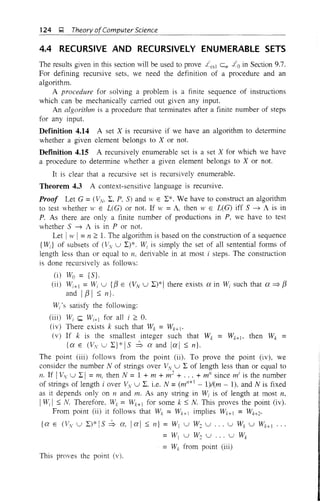
![Chapter 4: Formal Languages J;! 125
From the point (v) it follows that W E L(G) (i.e. S ~ w) if and only if
W E W~. Also. Wi, W2, •.• , Wk can be constructed in a finite number of steps.
We give the required algorithm as follows:
Algorithm to test whether w E L(G). 1. Construct Wi, W2• ... using the
points (i) and (ii). We terminate the construction when Wk+] = Wk for the first
time.
2. If yi' E Wk, then W E L(G). Otherwise, W E L(G). (As IWk Is N, testing
whether W is in Wk requires at most N steps.) I
EXAMPlE 4.18
Consider the grammar G given by S ~ OSA]2. S ~ 012, 2A) ~ A]2,
lA] ~ 11. Test whether (a) 00112 E L(G) and (b) 001122 E L(G).
Solution
(a) To test whether w =00112 E L(G), we construct the sets Wo, WI, W2
etc. Iwl = 5.
Wo= {S}
W] = {012, S, OSA]2}
Wo = {012, S, OSA I 2}
As W2 =WI, we terminate. (Although OSA]2 => 0012A]2, we cannot
include 0012A]2 in W] as its length is> 5.) Then 00112 E WI' Hence,
00112 E LCG).
(b) To test whether w =001122 E L(G). Here, Iw 1= 6. We construct Wo,
WI. W2, etc.
Wo= {S}
W] = {012. S, OSA]2}
Wo = {012, S, OSA]2, 0012A]2}
W3 = {OIl, S. OSA]2. 0012A]2, 001A]22}
W4 = {012. S, OSA]2, 0012A]2. 001A]22, 001122}
W5 = {012, S. OSA]2. 0012A]2, 001A]22. 001122}
As Ws = W4, we terminate. Then 001122 E W4. Thus. 001122 E L(G).
The following theorem is of theoretical interest, and shows that there
exists a recursive set over {O, I} which is not a context-sensitive language. The
proof is by the diagonalization method which is used quite often in set theory.
1 neorem 4.4 There exists a recursive set which is not a context-sensitive
language over {O, I}.
Proof Let 2: = {O, I}. We write the elements of 2:* as a sequence (i.e. the
elements of 2:* are enumerated as the first element, second element, etc.) For](https://image.slidesharecdn.com/automata-150510143406-lva1-app6891/85/Automata-138-320.jpg)
![126 Q Theory ofComputer Science
example, one such way of writing is A, 0, I, 00, 01, 10, 11, 000, .... In this
case. 010 will be the 10th element.
As every grammar is defined in terms of a finite alphabet set and a finite
set of productions, we can also write all context-sensitive grammars over 2.: as
a sequence, say Gj; G2, .•.•
We define X ={>Vi E 2.:* IWi r;z: L(G;)}. We can show that X is recursive.
If W E 2.:*, then we can find i such that W = >Vi' This can be done in a finite
number of steps (depending on IW 1). For example, if >v = 0100, then W = W20'
As G20 is context-sensitive, we have an algorithm to test whether vI' =W20 E
L(G20) by Theorem 4.3. So X is recursive.
We prove by contradiction that X is not a context-sensitive language. If it
is so, then X = L(G,,) for some n. Consider w" (the 11th element in 2.:*). By
definition of X, W n E X implies W n r;z: L(G,,). This contradicts X = L(Gn)·
W n r;z: X implies W n E L(Gn) and once again, this contradicts X = L(Gn). Thus,
X::t L(Gn) for any n. i.e. X is not a context-sensitive language. I
4.5 OPERATIONS ON LANGUAGES
We consider the effect of applying set operations on £0, £c51' ;[efl, elr!. Let
A and B be any two sets of strings. The concatenation AB of A and B is
defined by AB = {uv I U E A, v E B}. (Here, uv is the concatenation of the
strings u and v.)
We define Al as A and A,,+I as AliA for all n :::::: 1.
The transpose set AT of Ais defined by
AT = {Ill U E A}
Theorem 4.5 Each of the classes ;[0, , £ef); elr] is closed under union.
Proof Let L I and L2 be two languages of the same type i. We can apply
Theorem 4.1 to get grammars
and
of type i generating L] and L2• respectively. So any production in G] or G2
is either ex ~ {3, where ex, {3 contain only variables or A ~ a, where A E Vv,
a E 2.:.
We can further assume that V;v n V';; =0. (This is achieved by renaming
the variables of V'~ if they occur in V'N')
Define a new grammar Gli as follows:
Gil = (V'N U V'~, U {5}, 2.:] U 2.:2, PII' S)
where 5 is a new symboL i.e. 5 r;z: V'N U V',~
Pli = PI U P2 U {5 ~ 51' 5 ~ 52}](https://image.slidesharecdn.com/automata-150510143406-lva1-app6891/85/Automata-139-320.jpg)
![Chapter 4: Formal Languages ~ 127
*We prove L(G,,) = Ll U L2 as follows: If W E Lj U L2, then 5j => W or
52 => w. Therefore, G,
Go
*or 5 => 50 => w, l.e. W E L(G,,)
Gu Gu
Thus, L j U L2 ~ L(G,).
To prove that L(G,J ~ Ll U L2• consider a derivation of w. The first step
should be 5 ~ 5j or 5 ~ 52' If 5 ~ 51 is the first step, in the subsequent steps
5: is changed. As Vi.: (l V;": :f:- 0, these steps should involve only the variables
of V:v and the productions we apply are in Pj. So 5 ~ w. Similarly, if the
G,
first step is 5 ~ 52, then 5 => 52 ~ w. Thus, L(G,,) =Ll U L2. Also, L(G,J
G, G,
is of type 0 or type 2 according as L1 and L2 are of type 0 or type 2. If A
is not in L j U L2, then L(G,,) is of type 3 or type 1 according as Lj and L2
are of type 3 or type 1.
Suppose A E L j • In this case, define
G" = (V~, U V:v U {5, 5'}, I j U I2> P,!, 5')
where (i) S' is a new symbol, i.e. 5' e: V'N U V',~ U {5}, and (ii) P" =
Pi U P2 U {5' -? 5, 5 -? 5> 5 -? 52}' So, L(Gu ) is of type 1 or type 3
according as L] and L2 are of type 1 or type 3. When A E L2, the proof is
similar. I
Theorem 4.6 Each of the classes ,10, L es > L cf> ;irl is closed under
concatenation.
Proof Let L j and L2 be two languages of type i. Then, as in Theorem 4.5, we
get Gj = CV:v, I> Pl, 51) and G2 = (V':v , I:, P2, 52) of the same type i. We
have to prove that L1L: is of type i.
Construct a new grammar Geon as follows:
Geon =(V'N U V, U {5}, L1 U L2, Peon' 5)
where 5 e: V~v U V(
Peon = Pl U P2 U {5 -? 5i 52}
We prove L1L: = L(Geon)' If W = WjW: E LjL:, then
*51 => lVI'
G,
So,
*5 => 5152 => WjW2
Geoa Gcon
Therefore.](https://image.slidesharecdn.com/automata-150510143406-lva1-app6891/85/Automata-140-320.jpg)
![128 ];I, Theory ofComputer Science
If >t' E L(Gcon)' then the first step in the derivation of w is S ~ SIS2'
As V;v n V'~ = 0 and the productions in GI or G2 involve only the variables
*(except those of the form A ~ a), we have W = WIW', where S => WI and
* - G]
S ~ W2' Thus LIL2 =L(Gem,). Also, Gcon is of type 0 or type 2 according
as G1 and G2 are of type 0 or type 2. The above construction is sufficient when
G] and G2 are also of type 3 or type 1 provided A ~ L] U L2.
Suppose GI and G2 are of type 1 or type 3 and A E L] or A E Lo. Let
LIt =L1 - {A}, LI
2 =L2 - {A}. Then
{
L;L; U L;
L]L2 = L;L; u L;
L;L; u L; u L; u {A}
if A is in LI but not in L2
if A is in L2 but not in LI
if A is in L] and also in L:c
As we have already shown that L csi and 1'rl are closed under union, L IL2 is
of type 1 or type 3 according as L I and L2 are of type 1 or type 3.
Theorem 4.7 Each of the classes Lo, Lcslo Lcflo £rl is closed under the
transpose operation.
Proof Let L be a language of type i. Then L =L(G), where G is of type i.
We construct a new grammar CTas follows: GT=(VN> ~,pT, S), where the
productions of pT are constructed by reversing the symbols on L.R.S. and
R.R.S. of every production in P. Symbolically, cXt ~ f3T is in pT if a ~ f3 is
in P.
From the construction it is obvious that GT
is of type 0, 1 or 2 according
as G is of type 0, 1 or 2 and L(GT
) = LT. For regular grammar, the proof is given
in Chapter 5.
It is more difficult to establish the closure property under intersection at
present as we need the properties of families of languages under consideration.
We state the results without proof. We prove some of them in Chapter 8.
Theorem 4.8 (i) Each of the families Lo], Lcslo Lrl is closed under
intersection.
(ii) Let1 is not closed under intersection. But the intersection of a context-
free language and a regular language is context-free.
4.6 LANGUAGES AND AUTOMATA
In Chapters 7 and 9, we shall construct accepting devices for the four types
of languages. Figure 4.1 describes the relation between the four types of
languages and automata: TM, LBA, pda, and FA stand for Turing machine,
linear bounded automaton, pushdown automaton and finite automaton,
respectively.](https://image.slidesharecdn.com/automata-150510143406-lva1-app6891/85/Automata-141-320.jpg)
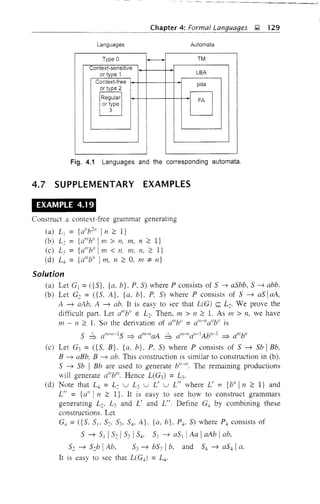
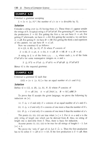


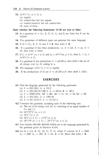
![4.5
4.6
4.7
4.8
4.9
4.10
4.11.
4.12.
4.13.
4.14.
4.15.
4.17.
Chapter 4: Formal Languages ~ 135
Find the language generated by the grammar 5 ~ AB, A ~ Alia,
B ~ 2B I3. Can the above language be generated by a grammar of
higher type?
State whether the following statements are true or false. Justify your
answer with a proof or a counter-example.
(a) If G] and G2 are equivalent then they are of the same type.
(b) If L is a finite subset of L*, then L is a context-free language.
(c) If L is a finite subset of L*, then L is a regular language.
Show that {a"
2
1 n :::: I} is generated by the grammar 5 ~ a, 5 ~ A3A4'
A3 ~ AlA~2> A 3 ~ AlA}, AlA} ~ aA2A l> Ala ~ aA t, A2a ~ aA2>
AlA, ~ A"a, A 2A4 ~ A 5a, A 2A 5 ~ A 5a, A 5 ~ a.
Construct (i) a context-sensitive but not context-free grammar, (ii) a
context-free but not regular grammar, and (iii) a regular grammar to
generate {a" 111 :::: I}.
Construct a grammar which generates all even integers up to 998.
Construct context-free grammars to generate the following:
(a) {all/I" 1m :;t 11, m, n:::: I}.
(b) {al
l/"e" lone of I, m, 11 equals 1 and the remaining two are equal}.
(c) {all/I" I 1 ::; m ::; 11}.
(d) {al
bli1
e"[1 + In =11}.
(e) The set of all strings over {a. I} containing twice as many O·s as
I's,
Construct regular grammars to generate the following:
(a) {a211
1n :::: I}.
(b) The set of all strings over {a. h} ending in a.
(c) The set of all strings over {a. b} beginning with a.
(d) {al
l/"e" II, m, n :::: I}.
(e) {(ab)"f n :::: I},
Is => an equivalence relation on (Vv u L)*?G .
Shmv that G] = ({5}, {a, b}, Pj, S), where p] = {S ~ a5blab} is
equivalent to G2 =({S, A, B. C}. {a, b}. P2, 5). Here P2 consists of
5 ~ AC, C ~ 5B. 5 ~ AB, A ~ a, B ~ b.
If each production in a grammar G has some variable on its right-hand
side, what can you say about L(G)?
Show that {abc, bca. eab} can be generated by a regular grammar
whose terminal set is {a, b, e}.
Construct a grammar to generate {(ab)"[II:::: I} u {(ba)"!n:::: I}.
Show that a grammar consisting of productions of the form A ~ xB Iy.
where x, yare in L* and A, B E Vv. is equivalent to a regular grammar.](https://image.slidesharecdn.com/automata-150510143406-lva1-app6891/85/Automata-148-320.jpg)

![Chapter 5: Regular Sets and Regular Grammars ~ 137
Notes: (1) We use x for a regular expression just to distinguish it from the
symbol (or string) x.
(2) The parentheses used in Rule 5 influence the order of evaluation of
a regular expression.
(3) In the absence of parentheses, we have the hierarchy of operations as
follows: iteration (closure). concatenation, and union. That is, in evaluating a
regular expression involving various operations. we perform iteration first, then
concatenation. and finally union. This hierarchy is similar to that followed for
arithmetic expressions (exponentiation. multiplication and addition).
DefInition 5.1 Any set represented by a regular expression is called a regular
set.
If for example, a, bEL. then (i) a denotes the set {a}, (ii) a + b denotes
{a, b}, (iii) ab denotes {ab}, (iv) a* denotes the set {A. a, aa. aaa, ...} and
(v) (a + b)* denotes {a, b}*.
The set represented by R is denoted by L(R),
Now we shall explain the evaluation procedure for the three basic
operations. Let R j and R: denote any two regular expressions. Then (i) a
string in L(Rj + R:) is a string from R] or a string from R:; (ii) a string in
L(Rj R2) is a string from R j followed by a string from R,. and (iii) a string
in L(R*) is a string obtained by concatenating 11 elements for some II 2: O.
Consequently. (i) the set represented by R j + R2 is the union of the sets
represented by R] and R2• (ii) the set represented by RjR: is the concatenation
of the sets represented by R j and R:. (Recall that the concatenation AB of sets
A and B of strings over I is given by AB = {H'(W: IWj E A, 1~': E B}, and
(iii) the set represented by R* is {WI"': ... It',JWi is in the set represented by
Rand Il 2: O.} Hence.
L(Rj + R2) = L(R]) u L(R2), L(R]R:) = L(RI)L(R:)
L(R*) = (L(R»)*
Also.
L(R*) = (L(R)* = U L(R)"
11=0
L(0) = 0, L(a) = {a}.
Note: By the definition of regular expressions, the class of regular sets over
I is closed under union, concatenation and closure (iteration) by the conditions
2. 3. 4 of the definition.
EXAMPLE 5.1
Describe the following sets by regular expressions: (a) {101 L (b) {abba},
(c'{OL 1O}, (d) {A. ab}, (e) {abb. a, b, bba}, (f) {A, 0, 00, 000.... J, and
(g) {1, 1L 11 L ... }.
Solution
(a) Now. {l}. {OJ are represented by 1 and O. respectively. 101 is obtained
by concatenating L 0 and L So. {1OI} is represented by 101.](https://image.slidesharecdn.com/automata-150510143406-lva1-app6891/85/Automata-150-320.jpg)
![138 &2 Theory ofComputer Science
(b) abba represents {abba}.
(c) As {01, 1O} is the union of {01} and {10}, we have {Ot 1O}
represented by 01 + 10.
(d) The set {A, ab} is represented by A + abo
(e) The set {abb, a, b, bba} is represented by abb + a + b + bba.
(f) As {A, 0, 00, 000, ... } is simply {O}*. it is represented by 0*.
(g) Any element in {L 11, 11 L ... } can be obtained by concatenating
1 and any element of {l}*. Hence 1(1)* represents {I, 11, Ill, ...}.
EXAMPLE 5.2
Describe the following sets by regular expressions:
(a) L 1 =the set of all strings of O's and l's ending in 00.
(b) L2 = the set of all strings of O's and l's beginning with 0 and ending
with 1.
(c) L3 ={A, 11, 1111, 111111, ... }.
Solution
(a) Any string in L] is obtained by concatenating any string over {O, I}
and the string 00. {O, I} is represented by 0 + 1. Hence L 1 is
represented by (0 + 1)* 00.
(b) As any element of L2 is obtained by concatenating 0, any stling over
{O, I} and 1, L2 can be represented by 0(0 + 1)* 1.
(c) Any element of L3 is either A or a string of even number of l's, i.e.
a string of the form (11)", 11 ~ O. So L3 can be represented by (11)*.
5.1.1 IDENTITIES FOR REGULAR EXPRESSIONS
Two regular expressions P and Q are equivalent (we write P =Q) if P and
Q represent the same set of strings.
We now give the identities for regular expressions; these are useful for
simplifying regular expressions.
II 0 + R =R
I, 0R = R0 = 0
13 AR =RA =R
14 A* = A and 0* = A
Is R+R=R
16 R*R* =R*
17 RR* = R*R
Is (R*)* =R*
19 A + RR* = R* = A + R*R
110 (PQ)*P = P(QP)*](https://image.slidesharecdn.com/automata-150510143406-lva1-app6891/85/Automata-151-320.jpg)

![142 ~ Theory ofComputer Science
EXAMPLE 5.6
Consider a graph (i.e. transItIOn system), contammg a A-move, given in
Fig. 5.3. Obtain an equivalent graph (i.e. transition system) without A-moves.
Fig. 5.3 Finite automaton of Example 5.6.
Solution
There is a A-move from qo to Q3' There are two edges, one from q3 to q2 with
label °and another from (]3 to q4 with label!. We duplicate these edges from
qo. As qo is an initial state. q3 is made an initial state. The resulting transition
graph is given in Fig. 5.4.
o
__~:GO
Fig. 5.4 Transition system for Example 5.6, without A-moves.
5.2.2 NDFAs WITH A-MOVES AND REGULAR EXPRESSIONS
In this section, we prove that every regular expression is recognized by a
nondeterministic finite automaton (NDFA) with A-moves.
Theorem 5.2 (Kleene's theorem) If R is a regular expression over L
representing L ~ L*. then there exists an NDFA M with A-moves such that
L = TUvll.
Proof The proof is by the pnnciple of induction on the total number of
characters in R. By 'character' we mean the elements of L, A, 0, * and +.
For example, if R =A + 10*11*0. the characters are A, +, 1, 0, *. 1, 1, *,
0, and the number of characters is 9.
Let L(R! denote the set represented by R.](https://image.slidesharecdn.com/automata-150510143406-lva1-app6891/85/Automata-155-320.jpg)
![Chapter 5: Regular Sets and Regular Grammars ~ 143
Basis. Let the number of characters in R be 1. Then R =A, or R = 0, or
R =ai, ai E I. The transition systems given in Fig. 5.5 will recognize these
regular expressions.
-O~~R =A R =$ R =8 i
Fig. 5.5 Transition systems for recognizing elementary regular sets.
Induction step. Assume that the theorem is true for regular expressions having
n characters. Let R be a regular expression having 11 + 1 characters. Then,
R=P+Q or R = PQ or R = p*
according as the last operator in R is +, product or closure. Also P and Q are
regular expressions having 11 characters or less. By induction hypothesis. L(P)
and L(Q) are recognized by M j and M: where M 1 and M: are NDFAs with
A-moves, such that L(P) = T(M j ) and L(Q) = T(M:). M j and M: are
represented in Fig. 5.6.
r
o
01
o
oFig. 5.6 Nondeterministic finite automata M1 and M2.
The initial state and the final states of M j and M: are represented in the usual
way.
Case 1 R =P + Q. In this case we construct an NDFA M with A-moves
that accepts L(P + Q) as fo11O'/s: qo is the initial state of M, qo not in M j
or M:. qj is the final state of M: once again q( not in M j or M:. M contains
all the states of M, and M: and also their transitions. We add additional
A-transitions from qo to the initial states of M1 and M: and from the final
states of M j and M: to qt. The NDFA M is as in Fig. 5.7. It is easy to see
that TUI1) = T(MJ u T(M2) = L(P + Q).
Case 2 R =PQ. In this case we introduce qo as the initial state of M and
qr as the final state of M. both qo, qr not in M] or M2. New A-transitions are
added between qo and the initial state of Mj • between final states of Mj and
the initial state of M2• and between final states of M: and the final state qr of
M. See Fig. 5.8.](https://image.slidesharecdn.com/automata-150510143406-lva1-app6891/85/Automata-156-320.jpg)
![144 l;.l Theory ofComputer Science
A
M2
Fig. 5.7 NDFA accepting L(P + Q).
A
A
M1 ~
Fig. 5.8 NDFA accepting L(PQ).
Case 3 R = (P)*. In this case, qo, q and qt are introduced. New A-transitions
are introduced from qo to q, q to qr, q to the initial state of M] and from the
final states of M] to q. See Fig. 5.9.
Thus in all the cases. there exists an NDFA M with A-moves, accepting
the regular expression R with n + 1 characters. By the principle of induction.
this theorem is true for all regular expressions. I
A
A
qo )------J l------JG
Fig. 5.9 NDFA accepting L(P*).](https://image.slidesharecdn.com/automata-150510143406-lva1-app6891/85/Automata-157-320.jpg)
![Chapter 5: Regular Sets and Regular Crammars &2 145
Theorem 5.1 gives a method of constructing NDFAs accepting P + Q, PQ
and P* using the NDFAs corresponding to P and Q. In the later sections we
give a method of converting NDFA M with A-moves into an NDFA M]
without A-moves and then into a DFA M 2 such that T(lv!) =T(M]) =T(M2).
Thus, if a regular expression P is given, we can construct a DFA accepting
UP).
The following theorem is regarding the converse. Both the Theorems 5.2
and 5.3 prove the equivalence of regular expressions or regular sets and the
sets accepted by deterministic finite automata.
Theorem 5.3 Any set L accepted by a finite automaton M is represented by
a regular expression.
Proof Let
M = ({ql ... q",}, L. 8, qj. F)
The construction that we give can be better understood in terms of the state
diagram of AI. If a string W E L* is accepted by M, then there is a path from
q] to some final state with path value w. So to each fmal state. say qi' there
corresponds a subset of L* consisting of path values of paths from qo to '7j'
As T(M) is the union of such subsets of L*. it is enough to represent them by
regular expressions. So the main part of the proof lies in the construction of
subsets of path values of paths from the state qi to the state qi'
Let Pi7 denote the set of path values of paths from qj to % whose
intermediate vertices lie in {qj, .. '. qd. We construct pb for k = 0, 1. ....
n recursively as follows:
p O={a E L 1 b(qj. a) = qi} (5.3)l.J
p.o ={a E L! 8(qi' a) = q;} U {A} (5.4)I!
pl; = pk-l (pk-l) * pH ,pH (5.5)1J Ik kk k) U I]
In terms of the state diagram, the construction can be understood better.
P;J simply denotes the set of path values (i.e. labels) of edges from qi to qi'
In p;7 we include A in addition to labels of self-loops from qi' This explains
(5.3) and (5.4).
Consider a path from qj to qi whose intermediate vertices lie in
{qj...., qd, If the path does not pass through qk' then its path value lies in
p;;-l. Othemise. the path passes through qk possibly more than once. The path
can be split into several paths with path values H.'l' H'2 ... 'VI as in Fig. 5.10.
W = 11'IW2 .. , WI' Wi is the path value of the path from qi to qk (without
passing through qk. i.e. qk is not an intermediate vertex). W2' . , ., 11'1-1 are the
path values of paths from qk to itself without passing through qk' WI is the path
value of the path from qk to qj without passing through q/:. So Wi is in p;Z-l.
W2' ,." WI_l are in (pA-i
). and WI is in Pk~-l. This explains (5.5).](https://image.slidesharecdn.com/automata-150510143406-lva1-app6891/85/Automata-158-320.jpg)
![146 g Theory of Computer Science
Fig. 5.10 A path from q, to qj'
We prove that the sets introduced by (5.3)-(5.5) are represented by
regular expressions by induction on k (for all i and j). P;J is a finite subset of
I.. say {aJ . ..., arlo Then. P;J is represented by PiJ =aJ + a2 + ... + at·
Similarly, we can construct p8 representing p;;. Thus, there is basis for
induction.
Let us assume the result for k - 1, i.e. p;;-l is represented by a regular
. p k- 1., all' d' F (5 ~) h pk pk-l (pk-l) '" pk-l pk-lexpresslOn ii lor 1 an j. rom..), we ave ij = ik kk "kj U ij •
S " b' h pk. d b pk pk-l(pk-J) '" pk-l pk-Io 1t IS 0 VIOUS t at ij IS represente Y ij = ik kk . kj U ij .
Therefore, the result is true for all k. By the principle of induction, the sets
constructed by (5.3)-(5.5) are represented by regular expressions.
As Q ={q J ••• " qlll}, prj denotes the set of path values of all paths from
11
ql to %. If F = {qii' ..., qr,,}, then T(M) = .~/y~. So T(N!) is represented
by the regular expression P{'f + ... + pn. Thus, L =T(M) is represented
by a regular expression.
Note: P;J and P;; are the subsets of I. U {A}, and so they are finite sets. So
every P;7 is obtained by applying union, concatenation and closure to the set
of all singletons in I. U {A}. Using this we prove Kleene's theorem (Theorem
5.4) at the end of this section. Kleene's theorem characterizes the regular sets
in terms of subsets of I. and operations (union, concatenation, closure) on
singletons in I. U {A}.
5.2.3 CONVERSION OF NONDETERMINISTIC SYSTEMS TO
DETERMINISTIC SYSTEMS
The construction we are going to give is similar to the construction of a DFA
equivalent to an ])1)FA and involves three steps.
Step 1 Convert the given transition system into state transition table where
each state corresponds to a row and each input symbol corresponds to a
column.
Step 2 Construct the successor table which lists the subsets of states
reachable from the set of initial states. Denote this collection of subsets by Qt.
Step 3 The transition graph given by the successor table is the required
deterministic system. The final states contain some final state of NDFA. If
possible. reduce the number of states.](https://image.slidesharecdn.com/automata-150510143406-lva1-app6891/85/Automata-159-320.jpg)
![Chapter 5: Regular Sets and Regular Grammars Q 147
Note: The construction is similar to that given in Section 3.7 for automata
except for the initial step. In the earlier method for automata, we started with
[qo]. Here we start with the set of all initial states. The other steps are similar.
EXAMPLE 5.7
Obtain the deterministic graph (system) equivalent to the transition system
given in Fig. 5.11.
I----a------{G
Fig. 5.11 Nondeterministic transition system of Example 5.7.
Solution
We construct the transition table corresponding to the given nondeterministic
system. It is given in Table 5.1.
TABLE 5.1 Transition Table for Example 5.7
StateII. a b
---<§J q1. q2
q1 qQ
@ qQ, q1
We construct the successor table by starting with [qo, qj]. From Table 5.1
we see that [qo, qj, q~] is reachable from [qo, qtJ by a b-path. There are no
a-paths from [qo, qtJ· Similarly, [qo, qd is reachable from [qQ, qj, q2] by an
a-path and [qo, qj, q2] is reachable from itself. We proceed with the
construction for all the elements in Q~
We terminate the construction when all the elements of Q' appear in the
successor table. Table 5.2 gives the successor table. From the successor table
it is easy to construct the deterministic transition system described by Fig. 5.12
TABLE 5.2 Deterministic Transition Table for Example 5.7
Q a b
[qQ. q,,] 0 [qQ. q1. q2]
[qQ, q1' q2] [qQ, q1] [qQ, q1, q2]
0 0 0](https://image.slidesharecdn.com/automata-150510143406-lva1-app6891/85/Automata-160-320.jpg)
![148 ~ Theory ofComputer Science
a a
b
Fig. 5.12 Deterministic transition system for Example 5.7.
as go and q2 are the final states of the nondeterministic system [qo, q]l and
kin, ql" q2] are the final states of the deterministic system.
5.2.4 ALGEBRAIC METHOD USING ARDEN'S THEOREM
The following method is an extension of the Arden's theorem (Theorem 5.1).
This is used to find the Le. recognized by a transition system.
The following assumptions are made regarding the transition system:
(i) The transition graph does not have A-moves.
(ii) It has only one initial state, say VI'
(iii) Its vertices are 1' .•• V".
(i) Vi the Le. represents the set of strings accepted by the system even
though v, is a final state.
(Y) (Xii denotes the I.e. representing the set of labels of edges from l'i to
1> When there is no such edge. aU == 0. Consequently, we can get the
following set of equations in Vi .. , V,,:
VI == Viall + V2a 21 + ... + Vila,,] + A
By repeatedly applying substitutions and Theorem 5.1 (Arden's theorem),
we can express Vi in terms of aii's.
For getting the set of strings recognized by the transition system, we have
to take the 'union" of all V;'s corresponding to final states.
EXAMPLE 5.R
Consider the transition system given in Fig. 5.13. Prove that the strings
recognized are (a + a(b + aa)*b)* arb + aa)* a.](https://image.slidesharecdn.com/automata-150510143406-lva1-app6891/85/Automata-161-320.jpg)
![Chapter 5: Regular Sets and Regular Grammars w 149
a b
Fig. 5.13 Transition system of Example 5.8.
Solution
We can directly apply the above method since the graph does not contain any
A-move and there is only one initial state.
The three equations for q]. q2 and q3 can be written as
ql = q]a + q2b + A, q2 = q]a + q2b + q3a. q3 = q2a
It is necessary to reduce the number of unknowns by repeated substitution. By
substituting q3 in the q2-equation. we get by applying Theorem 5.1
q2 =q]a + q2b + q2aa
= qla + q2(b + aa)
= qla(b + aa)*
Substituting q2 in ql' we get
ql =qla + qla(b + aa)*b + A
= ql(a + a(b + aa)*b) + A
Hence,
ql =A(a + a(b + aa)*b)*
q2 = (a + a(b + aa)*b)* a(b + aa)*
q3 = (a + a(b + aa)*b)* a(b + aa)*a
Since q3 is a final state, the set of strings recognized by the graph is given by
(a + a(b + aa)*b)*a(b + aa)*a
EXAMPLE 5.9
Prove that the finite automaton whose transitIOn diagram is as shown in
Fig. 5.14 accepts the set of all strings over the alphabet {a, b} with an equal
number of a's and b's, such that each prefix has at most one more a than the
b's and at most one more b than the a's.
a
b
b
a
a,b
Fig. 5.14 Finite automaton of Example 5.9.](https://image.slidesharecdn.com/automata-150510143406-lva1-app6891/85/Automata-162-320.jpg)

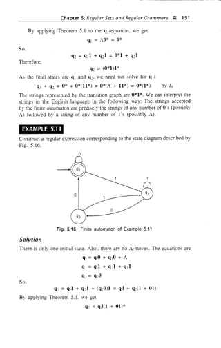
![152 g, Theory of Computer Science
Also,
q] =q10 + q30 + A =qIO + q200 + A
= q10 + (q11(1 + 01)*)00 + A
= ql(O + 1(1 + 01)* 00) + A
Once again applying Theorem 5.1, we get
ql = NO + 1(1 + 01)* 00)* = (0 + 1(1 + 01)* 00)*
As ql is the only final state, the regular expression corresponding to the given
diagram is (0 + 1(1 + 01)* 00)*.
EXAMPLE 5.12
Find the regular expression corresponding to Fig. 5.17.
o
oo
Gf------------i
o
Fig. 5.17 Finite automaton of Example 5.12.
Solution
There is only one initial state. and there are no A-moves. So, we form the
equations cOlTesponding to qj, q2, q3, q4:
ql = q10 + q30 + q40 + A
q2 = qll + q21 + q41
q3 = Q20
NOv.
Thus. we are able to write q" q4 in terms of q2' Using the qTequation, we
get](https://image.slidesharecdn.com/automata-150510143406-lva1-app6891/85/Automata-165-320.jpg)
*)
From the ql-equation, we have
ql =qlO + q200 + C12010 + A
= q]O + q2(00 + 010) + A
= q]O + q]l(l + 011)* (00 + 010) + A
Again, by applying Theorem 5. L we obtain
ql =A(O + 1(1 + 011)* (00 + 010»*
q.. = Q201 = q1l(1 + 011)* 01
= (0 + 1(1 + 011)*(00 + 010»*(1(1 + 011)* 01)
5.2.5 CONSTRUCTION OF FINITE AUTOMATA EQUIVALENT
TO A REGULAR EXPRESSION
The method we are going to give for constructing a finite automaton
equivalent to a given regular expression is called the subset method which
involves two steps.
Step 1 Construct a transition graph (transition system) equivalent to the
given regular expression using A-moves. This is done by using Theorem 5.2.
Step 2 Construct the transition table for the transition graph obtained in
step L Using the method given in Section 5.2.3, construct the equivalent DFA.
We reduce the number of states if possible.
. EXAMPLE 5.13
Construct the finite automaton equivalent to the regular expression
(0 + 1)*(00 + 11)(0 + 1)*
Solution
Step 1 (Construction of transitIon graph) First of all we construct the
transition graph with A-moves using the constructions of Theorem 5.2. Then
we eliminate A-moves as discussed in Section 5.2. L
We start vith Fig. 5.18(a).
V'le eliminate the concatenations in the given Le. by introducing new
vertices CJI and Ci2 and get Fig. 5.18(b).
We eliminate the'" operations in Fig. 5.18(b) by introducing two new
vertices Cis and CJ6 and the A-moves as shown in Fig. 5.18(c).
We eliminate concatenations and + in Fig. 5.18(c) and get Fig. 5.18(d).
We eliminate the A-moves in Fig.5.18(d) and get Fig. 5.18(e) which
gives the 1',TDFA equivalent to the gIven i.e.](https://image.slidesharecdn.com/automata-150510143406-lva1-app6891/85/Automata-166-320.jpg)
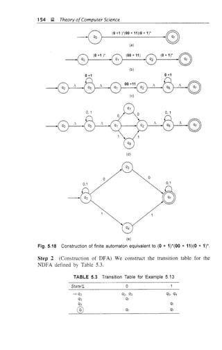
![- - - - - - - - - - - ---------
~~~-
Chapter 5: Regular Sets and Regular Grammars ~ 155
The successor table is constructed as given in Table 5.4.
TABLE 5.4 Transition Table for the DFA of Example 5.13.
o
---? [qQJ
[qQ, q3]
[qQ. q4]
[qQ. q3, qtl
[qQ. q4. qt]
OQ
[qQ, q31
[qQ, q3, qt]
[qQ, q3]
[qQ, q3· qtl
[qQ, q3· qt]
[qQ, q4]
[qQ, q4]
[qQ, q4, qfl
[qQ, q4, qfl
[qQ, q4, qtl
The state diagram for the successor table is the required DFA as described by
Fig. 5.19. As qf is the only final state of NDFA [qo, q3, qf] and [qo, % qf]
are the final states of DFA
Fig. 5.19 Finite automaton of Example 5.13.
Finally. we try to reduce the number of states. (This is possible when two
rows are identical in the successor table.) As the rows conesponding to
[qo, q3' qf] and [qo, q4' qf] are identical. we identify them. The state diagram
for the equivalent automaton. where the number of states is reduced, is
described by Fig. 5.20.
°
0,1
Fig. 5.20 Reduced finite automaton of Example 5.13.
Note: While constructing the transition graph equivalent to a given I.e., the
operation (concatenation. "'. +) that is eliminated first, depends on the regular
expresslon.](https://image.slidesharecdn.com/automata-150510143406-lva1-app6891/85/Automata-168-320.jpg)

![Chapter 5: Regular Sets and Regular Grammars ~ 157
Step 2 (Construction of DFA) For the NDFA given in Fig. 5.18(e). the
corresponding transition table is defined by Table 5.5.
TABLE 5.5 Transition Table for Example 5.14
StatelI 0
---0> qo q3 q1, q2
q1 qr
q2 q3
q3 q3 qr
®
The successor table is constructed and given in Table 5.6.
In Table 5.6 the columns corresponding to [qtJ and 0 are identical. So we
can identify [qtJ and 0.
TABLE 5.6 Transition Table of DFA for Example 5.14
Q Qo Q1
---0> [Qo] [q3] [q1, q2]
[q3] [q3] [qr]
[q1' Q2] [qrJ [q3]
@ 0 0
0 0 0
The DFA with the reduced number of states corresponding to Table 5.6
is defined by Fig. 5.22.
o
o
o
Fig. 5.22 Reduced DFA of Example 5.14.
5.2.6 EQUIVALENCE OF Two FINITE AUTOMATA
Tvo finite automata over L are equivalent if they accept the same set of strings
over L. When the two finite automata are not equivalent, there is some string](https://image.slidesharecdn.com/automata-150510143406-lva1-app6891/85/Automata-170-320.jpg)
![158 g Theory ofComputer Science
vI' over 2: satisfying the following: One automaton reaches a final state on
application of w, whereas the other automaton reaches a nonfinal state.
Ve give below a method. called the comparison method. to test the
equivalence of two finite automata over 2:.
Comparison Method
Let lVJ and 1);1' be two finite automata over 2:. Ve construct a comparison table
consisting of n + 1 columns. where n is the number of input symbols. The first
column consists of pairs of vertices of the form (q, q'), where q E M and q'
EM'. If (q, g') appears in some row of the first column, then the
corresponding entry in the a-column (a E 2:) is (q", q;'). where qa and q;' are
reachable from q and qt. respectively on application of a (i.e. by a-paths).
The comparison table is constructed by starting with the pair of initial
vertices qin. q(n of M and M'in the first column. The first elements in the
subsequent columns are (qa. q;,), where qa and q;' are reachable by a-paths
from qin and qili' We repeat the construction by considering the pairs in the
second and subsequent columns which are not in the first column.
The row-wise construction is repeated. There are tVO cases:
Case 1 If we reach a pair (q. q') such that q is a final state of M, and q' is
a nonfinal state of M' or vice versa, we terminate the construction and
conclude that l'Y1 and /vI' are not equivalent.
Case 2 Here the construction is tenninated when no new element appears in
the second and subsequent columns which are not in the first column (i.e.
when all the elements in the second and subsequent columns appear in the first
column). In this case we conclude that M and M' are equivalent.
EXAMPLE 5.1 5
ConSIder the fo]]owing two DFAs AI and M' over {O, I} given in Fig. 5.23.
Determine whether M and i'v1' are equivalent.
c
(a) (b)
Fig. 5.23 (a) Automaton M and (b) automaton M'.](https://image.slidesharecdn.com/automata-150510143406-lva1-app6891/85/Automata-171-320.jpg)

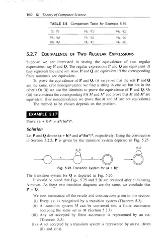


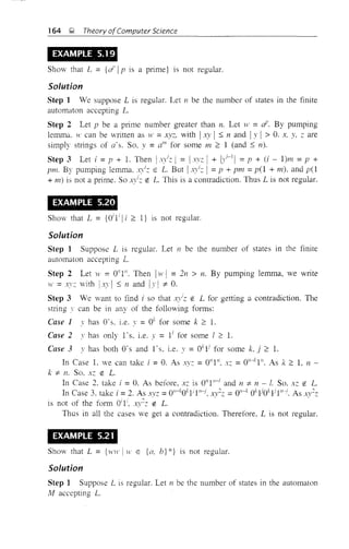


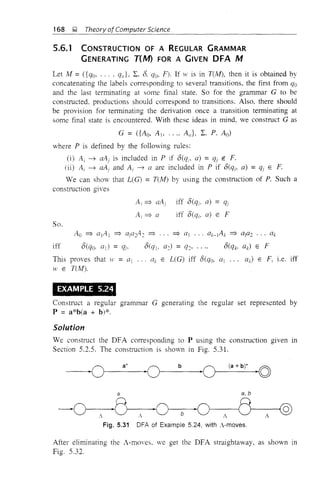
![Chapter 5: Regular Sets and Regular Grammars ~ 169
a a, b
r----b-l&Fig. 5.32 DFA of Example 5.24, without A-moves.
Let G = ({AO, Ad. {a. b}. P. Ao). where P is given by
Al ---+ a.
,"
~ll!
G is the required regular grammar.
5.6.2 CONSTRUCTION OF A TRANSITION SYSTEM M
ACCEPTING L(G) FOR A GIVEN REGULAR
GRAMMAR G
Let G =({Ao. AI' .... A,,}. L. P, Ao). We construct a transition system ,11,1
whose (i) states conespond to variables. (ii) initial state conesponds to Ao.
and (iii) transitions in :H conespond to productions in P. As the last
production applied in any derivation is of the form Ai ---+ a, the conesponding
transition terminates at a ne,' state. and this is the unique final state.
We define M as ({ qo- .... q/p qr}, L. O. qo, {qrD where <5 is defined as
follows:
(i) Each production Ai ---+aAi induces a transition from qi to CJi with
label a,
Each production Ak ---+ a induces a transition from qk to {fr with
label a.
From the construction it is easy to see that Ao =? alA] =? aja.:?A2 =? ...
=? aj ... a,,_jAn_] =? aj ... an is a derivation of ala.:? ... all iff there is a
path in M starting from qo and temlinating in CJr with path value aja.:? ... all"
Therefore. L(Gl = TUv1).
EXAMPLE 5.25
Let G =({Ao. Ad, {a. b}. P, Ao). where P consists of Ao ---+ aA j • Al ---+ bA I ,
A I ---+ a, A! ---+ bAa. Construct a transition system M accepting L(G).
Solution
Let Iv! =({CJCi. {fl' {ft}· {a. b}. 8. {fCi, {{ft})· where qo and qj correspond to Ao
and AI. respectively and Cit is the ne,v (final) state introduced. Ao ---+ aA j
induces a transition from {fo to q] with label a. Similarly. A] ---+ bAl and
AI ---+ bAI) induce transitions from CJj to {fj with label b and from ql to qo with](https://image.slidesharecdn.com/automata-150510143406-lva1-app6891/85/Automata-182-320.jpg)
![170 g Theorv ofComputer Science
label b, respectively. Al ~ a induces a transition from CJI to qf with label a.
M is given in Fig. 5.33.
b
~f--------a_00
b
Fig. 5.33 Transition system for Example 5.25.
EXAMPLE 5.26
If a regular grammar G is given by S ~ as Ia, find M accepting L(G).
Solution
Let qo correspond to 5 and qr be the new (final) state. M is given m
Fig. 5.34. Symbolically.
M = ({Cjo, qtl {a}. 8, C/o' {qr})
a
@~_a- 10 0
Fig. 5.34 Transition system for Example 5.26.
Note: If 5 ~ A is in P, the conesponding transition is from qo to qr with
label A.
By using the construction given in Section 5.2.3. we can construct a DFA
M accepting L(G) for a given regular grammar G.
5.7 SUPPLEMENTARY EXAMPLES
EXAMPLE 5.27
Find a regular expression conesponding to each of the following subsets of
{a. b}.
(a) The set of all strings containing exactly 2(/ s.
(b) The set of all strings containing at least 2a·s.
Ic) The set of all strings containing at most 2a's.
Cd) The set of a]] strings containing the substring aa.](https://image.slidesharecdn.com/automata-150510143406-lva1-app6891/85/Automata-183-320.jpg)
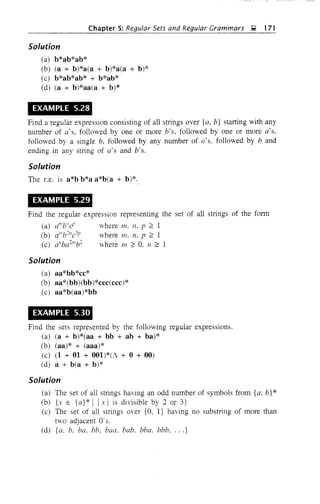

![Chapter 5: Regular Sets and Regular Grammars g 173
Then, >t' = 'VI' .. WI! where Wi E P*Q*. For simplicity take n = 2. (The result
can be extended by induction for any n). Then WJ = XIX2 .,. Xk' where
Xi E UP) and 11'2 =)'J)'2 ... )'1 where Yi E UQ), SO vI' =X1X2 ' , . XkY1Y2 ..• YI'
Each Xi or Yi is in L(P + Q). Hence 11' E L(P + Q)*, proving the first identity
in I] j. The second identity can be proved in a similar way.
Finally, we prove 112,
L((P + Q)R) = L(P + Q)L(R)
= (L(P) U L(Q»L(R)
UPR + QR) = L(PR) u L(QR)
=(L(P)L(R» u (L(Q)L(R»
But (A u B)C = AC u BC for A, B, C <;;;; L*. For. a string 11' in
(A u B)C is the concatenation of a string H'] in A or B and a string W2 in e.
If WI E A, then WjW2 E AC: if H'] E B, then WjW2 E Be. Hence W E AC u
Be. The other inclusion can be proved similarly. /12 follows from (A u B)e
= AC u Be.
EXAMPLE 5.34
Prove that P + PQ*Q =a*bQ* where P =b + aa*b and Q is any regular
expreSSiOn.
Proof L.H.S. = PA + PQ*Q
= peA + Q*Q)
= PQ*
= (b + aa*b)Q*
= (Ab + aa*b)Q*
= (A + aa*)bQ*
= a*bQ*
= R.H.S.
by h
by 112
by 19
by definition of P
by I,
by 1]2
by /')
EXAMPLE 5.35
Construct a regular grammar accepting L ={w E {a, b} * I W is a string over
{a. b} such that the number of b's is 3 mod 4}.
Solution
We construct a DFA M accepting L directly. The symbol a can occur in any
place in 11' and b has to occur in 4k + 3 places, where k 2': O. So we can have
stattOS q/, i =0, 1. 2, 3. for remembering that the string processed so far has
4k. 4k + L 4k + 2 and 4k + 3 b's (k 2': 0). q3 is the only final state. Also M
does not change state on reading a's. The state diagram representing M is
gIven in Fig. 5.35.](https://image.slidesharecdn.com/automata-150510143406-lva1-app6891/85/Automata-186-320.jpg)


![176 Q Theory ofComputer Science
State whether the following Statements 11-17 are true or false.
11. If L is finite then L* is finite.
12..Every finite subset of L* is a regular language.
13. Every regular language over L is finite.
14. a4
h3
is in the regular set given by a*(a + b)b*.
15. aa* + bb* is the same as (a + b)*.
16. The set of all strings starting with an a and ending in ah is defined by
the regular expression a(a + b)*b.
17. The regular expression (a + b)*c* is the same as a*(b + c)*.
EXERCISES
5.1 Represent the following sets by regular expressions:
(a) {O. 1. 2}.
(b) {1 21'+] In> O}.
(e) {'vI' E {a, b}* Iw has only one a}.
(d) The set of all strings over {O. 1} which has at most two zeros.
(e) {a2
, as. as, ... }.
(f) {d' In is divisible by 2 or 3 or n = 5}.
(g) The set of all strings over {a, b} beginning and ending with a.
5.2 Find all strings of length 5 or less in the regular set represented by the
following regular expressions:
(a) (ab + a)*(aa + b)
(b) (a*b + b*a)*a
(c) a* + Cab + a)*
5.3 Describe, in the English language, the sets represented by the following
regular expressions:
(a) a(a + b)*ab
(b) a*b + b*a
(c) (aa + b)*(bb + a)*
5.4 Prove the following identity:
(a*ab + ba)*a* = (a + ab + ba)*
5.5 Constmct the transition systems equivalent to the regular expressions
given in Exercise 5.2.
5.6 Constmct the transition systems equivalent to the regular expressions
given in Exercise 5.3.
5.7 Find the set of strings over L = {a, b} recognized by the transition
systems shown in Fig. 5.37(a-d).
5.8 Find the regular expression corresponding to the automaton given in
Fig. 5.38.](https://image.slidesharecdn.com/automata-150510143406-lva1-app6891/85/Automata-189-320.jpg)


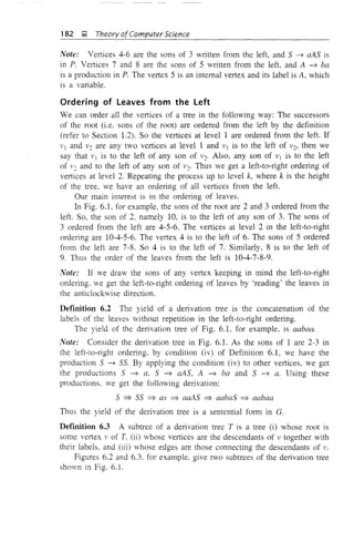
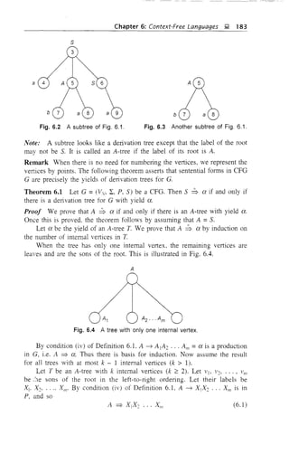
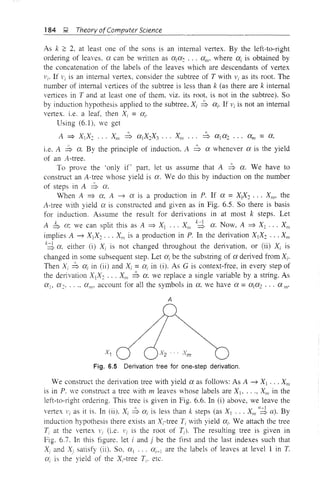
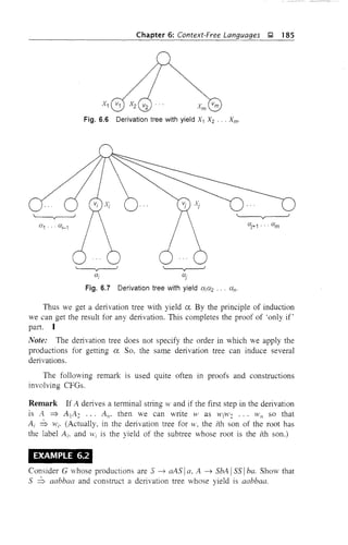


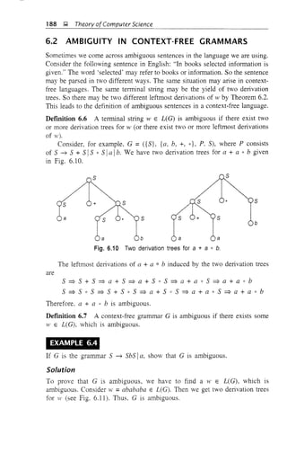

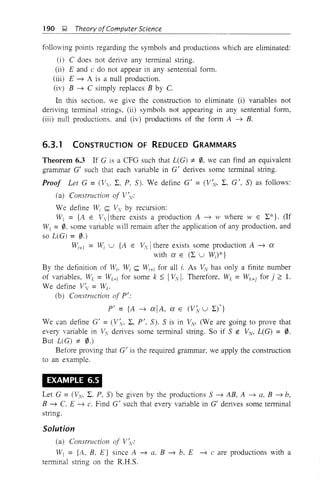
![Chapter 6: Context-Free Languages );,J 191
W~ = Wj U {AI E V:vlAj ----t a for some a E (2: U {A, B, E})*}
= tV] u {S} = {A~ B, E, S}
W3 =W~ U {AI E V:vlAI ----t a for some a E (2: U {S, A, B, E})*}
=W, U 0 = Wo
Therefore,
VN= {S. A. B, F}
(b) Construction of p':
P' = {AI ----t aIA[. a E (V:v U 2:)*}
= {S ----t AB, A ----t a, B ----t b, E ----t c}
Therefore.
G' = ({S, A, B, E}, {a, b. c}, P'. S)
Now we prove:
*
(i) If each A E V',. then A ::S w for some W E 2:*; conversely. if A ~ w,
, , G' G
then A E Vv,
(ii) L(G') = L(G),
To prove (i) we note that Wk = WI U W~ ... U Wk' We prove by
induction on i that for i = 1, 2..... k. A E Wi implies A ::S w for some
G'
W E 2:*. If A E Wj • then A ~ w. So the production A ----t w is in P'.
G
Therefore. A ::S lV. Thus there is basis for induction. Let us assume the result
G'
for i. Let A E Wi+l • Then either A E Wi' in which case. A ::S w for some
G'
w E 2:* by induction hypothesis. Or. there exists a production A ----t a with
a E (2: U wJ*. By definition of P'. A ----t a is in P'. We can write
a =XIX~ ... Xm, where Xj E 2: U Wi' If Xj E Wi by induction hypothesis.
Xl' ::S Wi for some Wi E 2:*. So, A ::S ~1)[W~ ... H'm E 2:* (when XI' is a terminaL
G' ' ' G ' ,
Wi =Xi)' By induction the result is true for i = 1. 2, ' ... k.
The converse part can be proved in a similar way by induction on the
number of steps in the derivation A ~ w. We see immediately that L(G') k
G
L(G) as V~. k V:v and P' k P, To prove L(G) k L(G'), we need an auxiliary
result
~:
A ::; w if A ~ w for some lV E 2:* (6.5)
G' G
We prove (6.5) by induction on the number of steps in the derivation A ~ W.
G
If 11 ~ w, then A ----t w is in P and A E W] k V'v. As A E V;v and vV E 2:*.
G
A ----t w is in P'. So A ~ w, and there is basis for induction. Assume (6.5)
G'
k+1
for derivations in at most k steps, Let A ~ w. By Remark appeating after
G](https://image.slidesharecdn.com/automata-150510143406-lva1-app6891/85/Automata-204-320.jpg)
![192 ~ Theory ofComputer Science
*
Theorem 6.1, we can split this as A ~ X]X2 ... XlIl ~ W(l-V2 ... 'Vm such
that Xj ~ H} If Xi E L, then Wj =Xj'
. G ' "
If Xj E VN then by (i), Xj E V~v. As Xj ~ Wj in at most k steps,
Xj ~ Wj' Also, Xl, X2, XlIl E (L U V~v)* implies that A ~ XlX2 ... XI1l is
in P'. Thus, A ~ XIX~ ... XlIl ::b WlW2 ... Will' Hence by induction, (6.5)
G' - G ' . •
is true for all derivations. In particular, S ~ W implies S => w. This proves
G G'
that L(G) ~ L(G'), and (ii) is completely proved. I
Theorem 6.4 For every CFG G = (VN, L, P, S), we can construct an
equivalent grammar G' =(VN, L', p', S) such that every symbol in 1"1 U L'
appears in some sentential form (i.e. for every X in V:v U L' there exists a
such that S ::b a and X is a symbol in the string a).
G'
Proof We construct G' = (V'N' L', P', S) as follows:
(a) Construction of Wi for i ?: 1:
(i) WI = IS}.
(ii) Wi+l =Wi U {X E 1v U L I there exists a production A ~ a with
A E Wi and a containing the symbol X}.
We may note that Wi ~ v'v uLand Wi ~ Wi+l • As we have only a finite
number of elements in VN U L, Wk = Wk+1 for some k. This means that
Wk =Wk+j for all j ?: O.
(b) Construction of VN, L' and p':
We define
VN= Vv (l Wk, L' = L U Wk
P'= {A ~ alA E Wk }.
Before proving that G' is the required grammar, we apply the construction to
an example.
EXAMPLE 6.6
Consider G =({S, A, B, E}, {a, b, c}, P, S), where P consists of S ~ AB,
A ~ a, B ~ b, E ~ c.
Solution
WI = IS}
W2 = IS} U {X E !y U L I there exists a production A ~ a with
A E WI and a containing X}
= IS} U {A, B}](https://image.slidesharecdn.com/automata-150510143406-lva1-app6891/85/Automata-205-320.jpg)
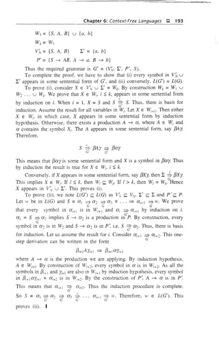
![194 g Theory of Computer Science
Definition 6.8 Let G = (VN, L, P, S) be a CFG. G is said to be reduced or
non-redundant if every symbol in VN U L appears in the course of the
delivation of some terminal string, i.e. for every X in v'v U L, there exists
a delivation S ::S aX[3 ::S W E L(G). (We can say X is useful in the
derivation of terminal strings.)
Theorem 6.5 For every CFG G there exists a reduced grammar G' which is
equivalent to G.
Proof We construct the reduced grammar in two steps.
Step 1 We construct a grammar Gj equivalent to the given grammar G so
that every variable in Gj derives some terminal string (Theorem 6.3).
Step 2 We construct a grammar G' = (V~v, L', p', S) equivalent to Gj so that
every symbol in G' appears in some sentential form of G' which is equivalent
to Gj and hence to G. G' is the required reduced grammar.
By step 2 every symbol X in G' appears in some sentential form, say
exX[3. By step 1 every symbol in exX[3 derives some terminal string. Therefore,
S ::S exX[3 ::S >t' for some w in L*, i.e. G' is reduced.
Note: To get a reduced grammar, we must first apply Theorem 6.3 and then
Theorem 6.4. For, if we apply Theorem 6.4 first and then Theorem 6.3, we may
not get a reduced grallli'1lar (refer to Exercise 6.8 at the end of the chapter).
EXAMPLE 6.7
Find a reduced grammar equivalent to the grammar G whose productions are
C ~ aBlbA ~ a.B ~ BClAB,S ~ ABICA,
Solution
Step 1 WI = {A, C} as A ~ a and C ~ b are productions with a terminal
string on R.H.S.
W~ = {A. C} U {AIIA I ~ ex with ex E (L U {A, C})*}
= {k C} U {S} as we have S ~ CA
W3 = {A, C, S} U {AI IAl ~ ex with ex E (L U {S, A, C})*}
= {A~ C~ S} u 0
v~v= W~ = {S, A, C}
p' = {A j ~ ex IAj, ex E (V~", U L)*}
= {S ~ CA. A ~. a, C ~ b}
Thus.
G] = ({S, A. C}. {a, b}, {S ~ CA, A ~ a, C ~ b}, S)](https://image.slidesharecdn.com/automata-150510143406-lva1-app6891/85/Automata-207-320.jpg)


![Chapter 6: Context-Free Languages ~ 197
R.H.S. of A ~ Xj X2 ••• Xk or by erasing some or all nullable variables
provided some symbol appears on the R.H.S. after erasing.
Let Gj =CV:v, 2.:, pI, S). G] has no null productions.
Before proving that G] is the required grammar, we apply the construction
to an example.
EXAMPLE 6.9
Consider the grammar G whose productions are S ~ as IAS, A ~ A,
S ~ A, D ~ b. Construct a grammar G] without null productions generating
L(G) - {A}.
Solution
Step 1 Construction of the set W of all nullable variables:
Wj = {AI E Vv IAj ~ A is a production in G}
= {A, B}
W2 = {A, B} u {S} as S ~ AB is a production with AS E wt
= {S, A, B}
W3 = W, U 0= w,
Thus.
W =W2 ={S, A, B}
Step 2 Construction of pI:
(i) D ~ b is included in pl.
(ii) S ~ as gives rise to S ~ as and S ~ a.
(iii) S ~ AB gives rise to S ~ AB, S ~ A and S ~ B.
(Note: We cannot erase both the nullable variables A and Bin S ~ AB as we
will get S ~ A in that case.)
Hence the required grammar without null productions is
Gj = ({S, A, B. D}.{a, b}. P, S)
where pI consists of
D ~ b, S ~ as. S ~ AS, S ~ a, S ~ A, S ~ B
Step 3 L(Gj ) =L(G) - {A}. To prove that L(G) =L(G) - {A}, we prove
an auxiliary result given by the following relation:
For all A E Vv and >1,' E 2.:*,
A ~ w if and only if A ~ >1,' and w ~ A
G, G
(6.6)
We prove the 'if part first. Let A ~ wand Ii' ;f. A. We prove that A ~ w
G G
by induction on the number of steps in the derivation A ~ w. If A => HI ~nd
G G](https://image.slidesharecdn.com/automata-150510143406-lva1-app6891/85/Automata-210-320.jpg)
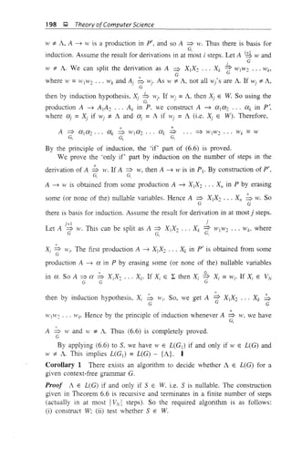

![200 l;l Theory ofComputer Science
(Actually, (ii) covers (i) as A E W(A)). Now, we define GI =(VN, ~, PI'S),
where PI is constructed using step 2 for every A E ~v.
Before proving that G] is the required grammar, we apply the construction
to an example.
EXAMPLE 6.10
Let G be S ~ AB, A ~ a. B ~ C Ib, C ~ D, D ~ E and E ~ a. Eliminate
unit productions and get an equivalent grammar.
Solution
Step 1 V;'o(S) = {S}, Wj(S) = WoeS} u 0
Hence W(S} = {S}. Similarly,
W(A} = {A}, Wee} = {E}
Wo(B} = {B}, WI(B) = {B} u {C} = {B, C}
W2(B) = {B. C} u {D}. W3(B) = {B, C, D} u {E}, W4(B} = W3(B}
Therefore,
W(B} = {B, C, D, E}
-Similarly,
Wo(C) = {C},
Therefore.
Hence,
W(C) = {C, D, E}, Wo(D} = {D}
Thus.
WeD} ={D, E}
in G',
Step 2 The productions in Gj are
S ~ AB. A ~ a.
B ~ b Ia, C ~ a,
By construction. G] has no unit productions.
To complete the proof we have to show that L(G'} = L(GI }.
Step 3 L(G') =L(G}. If A ~ a is in PI - P, then it is induced by B ~ a
in P with B E W(A}, a eo Vv. B E W(A} implies A ~ B. Hence, A ~ B
. ~ ~
=> a. So, if A => a, then A ~ a. This proves L(Gj } ;;; L(G'}.
G' G, G'
To prove the reverse inclusion, we start with a leftmost derivation
S => al => ao , .. => an = w
G G - G](https://image.slidesharecdn.com/automata-150510143406-lva1-app6891/85/Automata-213-320.jpg)
![Chapter 6: Context-Free Languages ,!;l, 201
,i;
Let i be the smallest index such that Cti ~ Cti+1 is obtained by a unit
production and j be the smallest index greater than i such that Ctj ~ Cti+J is
x G
obtained by a nonunit production. So, S ~ ai, and aj ~ aJ'+1 can be
G, ' G' .
written as
ai = H'iA;{3i =} wiAi+!f3i =} .. , =} WiAjf3i =} wir f3i = CXj+!
Aj E W(Ai) and Aj ~ ris a nonunit production. Therefore, Aj ~ r is a
production in PI' Hence, Ctj ~ aj+I' Thus, we have S ~ aj+I'
. G, ' G,
Repeating the argument whenever some unit production occurs in the
remaining part of the derivation, we can prove that S ~ a" = w, This proves
G,
L(G') s;;;; L(G). I
Corollary If G is a context-free grammar, we can construct an equivalent
grammar G' which is reduced and has no null productions or unit productions.
Proof We construct G] in the following way:
Step 1 Eliminate null productions to get G] (Theorem 6.6 or Corollary 2 of
this theorem).
Step 2 Eliminate unit productions in G] to get G2 (Theorem 6.7).
Step 3 Construct a reduced grammar G' equivalent to G] (Theorem 6.5). G'
is the required grammar equivalent to G.
Note: We have to apply the constructions only in the order given in the
corollary of Theorem 6.7 to simplify grammars. If we change the order we
may not get the grammar in the most simplified form (refer to Exercise 6.11).
6.4 NORMAL FORMS FOR CONTEXT-FREE GRAMMARS
In a context-free grammar. the R.H.S. of a production can be any string of
variables and terminals. When the productions in G satisfy certain restrictions,
then G is said to be in a 'normal form'. Among several 'normal forms' we study
two of them in this section-the Chomsky normal form (CNF) and the
Greibach nOlmal form.
6.4.1 CHOMSKY NORMAL FORM
In the Chomsky normal form (CNF). we have restrictions on the length of
R.H.S. and the nature of symbols in the R.H.S. of productions.
DefInition 6.11 A context-free grammar G is in Chomsky normal form if
every production is of the form A ~ G, or A ~ Be, and S ~ A is in G if](https://image.slidesharecdn.com/automata-150510143406-lva1-app6891/85/Automata-214-320.jpg)
![202 Q Theory ofComputer Science
A E L(G). When A is in L(G), we assume that S does not appear on the
RH.S. of any production.
For example, consider G whose productions are S ~ AB IA, A ~ a,
B ~ b. Then G is in Chomsky normal form.
Remark For a grammar in CNF, the derivation tree has the following
property: Every node has atmost two descendants-either two internal vertices
or a single leaf.
When a grammar is in CNF, some of the proofs and constructions are
simpler.
Reduction to Chomsky Normal Form
Now we develop a method of constructing a grammar in CNF equivalent to a
given context-free grammar. Let us first consider an example. Let G be S ~
ABC IaC, A ~ a. B ~ b, C ~ c. Except S ~ aC IABC, all the other
productions are in the form required for CNF. The terminal a in S ~ aC can
be replaced by a new variable D. By adding a new production D ~ a, the effect
of applying S ~ aC can be achieved by S ~ DC and D ~ a. S ~ ABC is not
in the required form. and hence this production can be replaced by S ~ AE and
E ~ Be. Thus, an equivalent grammar is S ~ AE IDC, E ~ BC, A ~ a,
B ~ b. C ~ c, D ~ a.
The techniques applied in this example are used in the following theorem.
Theorem 6.8 (Reduction to Chomsky normal form). For every context-free
grammar, there is an equivalent grammar G2 in Chomsky normal form.
Proof (Construction of a grammar in CNF)
Step 1 Elimination of null productions and unit productions:
We apply Theorem 6.6 to eliminate null productions. We then apply
Theorem 6.7 to the resulting grammar to eliminate chain productions. Let the
grammar thus obtained be G = (V"" L, P, S).
Step 2 Elimination of terminals on R.H.S.:
We define G1 =(V"" L, PI, S'), where p] and V;,vare constructed as follows:
(i) All the productions in P of the form A ~ a or A ~ BC are included
in Plo All the variables in Vv are included in V;",.
(ii) Consider A ~ Xj X2 ..• Xn with some terminal on RH.S. If Xi isa
terminaL say ai, add a new variable Ca to V;", and Ca ~ ai to Pl'
I I
In production A ~ Xj X2 ... Xii' every terminal on R.H.S. is replaced
by the corresponding new variable and the variables on the RH.S. are
retained. The resulting production is added to p]. Thus, we get
G1 = (V:"', L, Ph S).
Step 3 Restricting the number of variables on R.H.S.:
For any production in Plo the R.H.S. consists of either a single terminal (or](https://image.slidesharecdn.com/automata-150510143406-lva1-app6891/85/Automata-215-320.jpg)

![204 J;l Theory ofComputer Science
Let W E L(Gj ). To show that W E L(G), it 1S enough to prove the
following:
(6.7)
*We prove (6.7) by induction on the number of steps in A => w.
G,
If A => w, then A ---+ H' is a production in Pl' By construction of Pj, .v is
G,
a single terminal. So A ---+ W is in P, i.e. A => w. Thus there is basis for
induction. G
Let us assume (6.7) for derivations in at most k steps. Let A ~ w. We can
G,
split this derivation as A => A]A2 . .. Alii !b W] . W m = W such that Ai ~ Wi'
~ ~ ~
*Each Ai is either in Vy or a new variable, say C", When Ai E VN, Ai => Wi
• 1 ~
~,'
is a derivation in at most k steps. and so by induction hypothesis, Ai => Wi'. . . G
When Ai = C"i' the production CUi ---+ ai is applied to get Ai ::S Wi' The
production A ---+ A j A2 ... Alii is induced by a production A ---+ Xj X2 .•• XIII
in P where Xi = Ai if Ai E VN and Xi = Wi if Ai = CUI' So A => Xj X2 ... XIII
G
b H'jH'2 ... Wm' i.e. A b w. Thus, (6.7) is true for all derivations.
G G
Therefore. L(G) = L(G]).
The effect of applying A ---+ A j A2 •.. Am in a derivation for W E L(Gj )
can be achieved by applying the productions A ---+ A] Cl , Cl ---+ A2C2,
Cm- 2 ---+ Am-lAm in P2' Hence it is easy to see that L(GI ) <;;;; L(G2).
To prove L(Gc) <;;;; L(Gj ), we can prove an auxiliary result
A=>w
G,
if A E V;v, A => tV
G.
(6.8)
Condition (6.8) can be proved by induction on the number of steps in A => w.
G,
Applying (6.7) to S. we get L(G2) <;;;; L(G). Thus.
L(G) = L(G j ) = L(G2) I
EXAMPLE 6.12
Find a grammar in Chomsky normal form equivalent to S ---+ aAbB, A ---+
aAla. B ---+ bBlb.](https://image.slidesharecdn.com/automata-150510143406-lva1-app6891/85/Automata-217-320.jpg)
![Chapter 6: Context-Free Languages J;! 205
Solution
As there are no unit productions or null productions, we need not carry out
step 1. We proceed to step 2.
Step 2 Let Gj = (V'y {a, b}, PI' S), where Pj and V:v are constructed as
follows:
(i) A ~ a, B ~ b are added to Pl'
(ii) S ~ aAbB, A ~ aA, B ~ bB yield S ~ CaACbB. A ~ CaA.
B ~ C;,B. C{/ ~ a. Cb ~ b.
V'v = {S, A, B, C", Cb }·
Step 3 PI consists of S ~ CaACbB, A ~ CaA, B ~ C;,B, Ca ~ a.
Cb ~ b, A ~ a, B ~ b.
S ~ C{/AC/JB is replaced by S ~ CaC] , C1 ~ AC~. Ce ~ CbB
The remaining productions in Pj are added to Pc. Let
G: = ({S. A. B. CO' C/J' CI' Ce}, {a, b}, Pc. S),
where Pc consists of S ~ CaCjo Ci ~ ACe, Ce ~ C/JB, A ~ CaA. B ~ C/JB.
Ca ~ a, Cb ~ b. A ~ a. and B ~ b.
G: is in C:I'<'F and equivalent to the given grammar.
,
EXAMPLE 6.13
Find a grammar in C:I'<'F equivalent to the grammar
Solution
S ~ -S I[s :::J) S] Ipi q (S being the only variable)
As the given grammar has no unit or null productions, we omit step 1 and
proceed to step 2.
Step 2 Let Gj = (V, L. PI' S). where Pj and V~ are constructed as fonows:
(i) S ~ pi q are added to Pj.
(ii) S ~ - S induces S ~ AS and A ~ -.
(iii) S ~ [S :::J S] induces S ~ BSCSD, B ~ [,C ~ :::J. D ~]
1' = {So A. B. C. D}
Step 3 Pj consists of S ~ plq. S ~ AS. A ~ -, B ~ LC ~:::J, D ~].
S ~ BSCSD.
S ~ BSCSD is replaced by S ~ BCI , Cj ~ SCe' Ce ~ CC3, C3 ~ SD.
Let
Ge =({S, A. B. C. D, CI , C:, C3 }. L, Pc, S)
where P: consists of S ~ plq[AS[BCj , A ~ -, B ~ [. C ~ :::J, D ~],
CI ~ SCe' C: ~ CC3, C3 ~ SD. G: is in CNF and equivalent to the given
grammar.](https://image.slidesharecdn.com/automata-150510143406-lva1-app6891/85/Automata-218-320.jpg)
![206 g Theory ofComputer Science
6.4.2 GREIBACH NORMAL FORM
Greibach normal form (GNF) is another normal form quite useful in some
proofs and constructions. A context-free grammar generating the set accepted
by a pushdown automaton is in Greibach normal form as will be seen in
Theorem 7.4.
Deflnition 6.12 A context-free grammar is in Greibach normal form if every
production is of the form A ~ aa. where a E vt and a E L(a may be A),
and S ~ A is in G if A E L(G). When A E L(G), we assume that S
does not appear on the R.H.S. of any production. For example, G given by
S ~ aAB IA, A ~ bC, B ~ b, C ~ c is in GNF.
Note: A grammar in GNF is a natural generalisation of a regular grammar.
In a regular grammar the productions are of the form A ~ aa, where a E L
and a E Vv U {A}, i.e. A ~ aa, with avt and 1al s 1. So for a grammar
in GNF or a regular grammar, we get a (single) terminal and a string of
variables (possibly A) on application of a production (with the exception of
S ~ A).
The construction we give in this section depends mainly on the following
tVO technical lemmas:
Lemma 6.1 Let G = (Vy , L. P. S) be a CFG. Let A ~ Bybe an A-production
in P. Let the B-productions be B ~ f3j 11321 ... I13,. Define
P j =(P - {A ~ By}) U {A ~ f3iyl1 sis s}.
Then. Gj =(Vy , L, Pj, S) is a context-free grammar equivalent to G.
Proof If we apply A ~ By in some derivation for ]V E L(G), we have to
*
apply B ~ f3i for some i at a later step. So A 'Z' Biy. The effect of applying
A ~ By and eliminating B in grammar G is the same as applying A ~ f3iY
for some i in grammar G!. Hence H' E L(G!), i.e. L(G) s;;; L(G!). Similarly,
instead of applying A ~ f3iY. we can apply A ~ By and B ~ f3i to get
A ~ f3iY. This proves L(G]) s;;; L(G). I
G
Note: Lemma 6.1 is useful for deleting a variable B appearing as the first
symbol on the R.H.S. of some A-production, provided no B-production has B
as the first symbol on R.H.S.
The construction given in Lemma 6.1 is simple. To eliminate B in A ~ By,
we simply replace B by the right-hand side of every B-production.
For example. using Lemma 6.1. we can replace A ~ Bab by A ~ aAab,
A ~ bBab, A ~ aaab. A ~ ABab when the B-productions are B ~ aA 1 bB I
aaiAB.
The lemma is useful to eliminate A from the R.H.S. of A ~ Aa.
Lemma 6.2 Let G = (Vy , L, P, S) be a context-free grammar. Let the set
of A-productions be A ~ Aa! I... Aa, 11311 ... 113, (f3i'S do not start with A).](https://image.slidesharecdn.com/automata-150510143406-lva1-app6891/85/Automata-219-320.jpg)
![Chapter 6: Context-Free Languages ~ 207
Let Z be a new variable. Let G1 = (Vv u {ZL l:, PI' S), where PI is defined
as follows:
(i) The set of A-productions in PI are A ~ f3! If321 ... !f3s
A ~ f31 Z If32Z I ... lf3sZ
(ii) The set of Z-productions in PI are Z ~ a1 la2! ... !ar
Z ~ a1Z I a2Z ... !a,Z
(iii) The productions for the other variables are as in P. Then G! is a CFO
and equivalent to G.
Proof To prove L(G) ~ L(G), consider a leftmost derivation of H' in G. The
only productions in P - PI are A ~ AaI! Aa2 ... IA a,. If A ~ Aail'
A ~ Aai2, ..., A ~ Aah are used, then A ~ f3j should be used at a later
stage (to eliminate A). So we have A %f3;Aail ... ail while deriving w in
G. However. .
l.e.
.A => f3jAail ... ai;
G]
Thus. A can be eliminated by using productions in Gl. Therefore, w E L(G!).
To prove L(G)) ~ UG). consider a leftmost derivation of lV in G!. The
only productions in PI - P are A ~ f31ZI f32ZI ... lf3sZ. Z ~ all· .. la"
Z ~ ajZ Ia2Z I ... Ia,z. If the new variable Z appears in the course of the
derivation of 11', it is because of the application of A ~ f3jZ in some earlier
step. Also. Z can be eliminated only by a production of the form Z ~ ~ or
*Z ~ aJZ for some i and j in a later step. So we get A => f3J·ai ai ... ai. 1 2 k
~]
in the course of the derivation of w. But, we know that A => f3Pil ai2 ... aik
'
e
Therefore. W E L(G).
EXAMPLE 6.14
Apply Lemma 6.2 to the following A-productions in a context-free grammar
G.
A ~ aBD IbDB Ie A ~ ABIAD
Solution
In tL..; example. al = B. a2 = D, f31 = aBD. f32 = bDB, f33 = c. So the new
productions are:
(i) A ~ aBDlbDBlc.
(ii) Z ~ B, Z ~ D.
A ~ aBDZI bDBZI cZ
Z ~ BZIDZ](https://image.slidesharecdn.com/automata-150510143406-lva1-app6891/85/Automata-220-320.jpg)

![Chapter 6: Context-Free Languages J;;! 209
An_I-productions are in the required form. We repeat the construction by
considering An- 2• An- 3, .... A I'
Step 5 Modify Z;-productions. Every time we apply Lemma 6.2, we get a
new vfu'iable. (We take it as Z; when we apply the Lemma for ArProductions.)
The Zrproductlons are of the form Zi ~ aZi or Z; ~ a (where a is obtained
from Ai ~ Aia), and hence of the form Zi ~ ayor Zi ~ Aky for some k.
At the end of step 4. the R.H.S. of any Acproduction stmts with a terminal.
So we can apply Lemma 6.1 to eliminate Zi ~ Aky- Thus at the end of
step 5, we get an equivalent grammar G] in GNF.
It is easy to see that G] is in Gli'F. We start with G in CNG. In G any
A-production is of the form A ~ a or A ~ AB or A ~ CD. When we apply
Lemma 6.1 or Lemma 6.2 in step 2, we get new productions of the form
A ~ aa or A ~ [3, where a E V~ and [3 E V~y and a E L. In steps 3-5.
the productions are modified to the form A ~ aa or Z ~ a'a'. where a. a'
ELand a. a/ E V'(,.
Case 2 Construction of G when .A E L:
By the previous construction we get G' = (V~" L. Pl' 5) in GNF such that
L(G') =L - {A}. Define a new grammar GI as
GI = (Vy u {5'}, L. PI U {5' ~ 5. 5' ~ A}. 5')
5' ~ 5 can be eliminated by using Theorem 6.7. As 5-productions are in the
required form, 5'-productions are also in the required form. So L(G) =L(G])
and G] is in GNF. I
Remark Although we convert the given grammar to CNF in the first step.
it is not necessary to convert all the productions to the form required for CNF.
In steps 2-5. we do not disturb the productions of the form A ~ aa. a E L
and a E V. So such productions can be allowed in G (in step 1). If we apply
Lemma 6.1 or 6.2 as in steps 2-5 to productions of the form A ~ a. where
a E vt and Ia I;:: 2. the resulting productions at the end of step 5 are in the
required form (for GNF). Hence we can allow productions of the form A ~ a,
where a E V~. and Ia I ;:: 2.
Thus we can apply steps 2-5 to a grammar whose productions are either
A ~ aa where a E V. or A ~ a E V'(, where Ia I ;:: 2. To reduce the
productions to the form A ~ a E V. where Ia I;:: 2, we can apply step 2
of Theorem 6.8.
EXAMPLE 6.1 5
Construct a grammar in Greibach normal form equivalent to the grammar
5 -'t AA I a. A ~ 55 Ib.
Solution
The given grammar IS in C1'IF. 5 and A are renamed as A] and A2•
respectively. So the productions are A 1 ~ A IA2 1 a and A 2 ~ A]A 11 b. As the](https://image.slidesharecdn.com/automata-150510143406-lva1-app6891/85/Automata-222-320.jpg)
![21 0 .~ Theory ofComputer Science
given grammar has no null productions and is in CNF we need not carry out
step 1. So we proceed to step 2.
Step 2 (i) AI-productions are in the required fonn. They are Al ~ A2A2 1 a.
(ii) A2 ~ b is in the required fonn. Apply Lemma 6.1 to A2 ~ AjAj.
The resulting productions are A2 ~ A2A2A I, A2 ~ aA I • Thus the
ATproductions are
A2 ~ A2A2Aj, A2 ~ aA], Ao ~ b
Step 3 We have to apply Lemma 6.2 to ATProductions as we have
A 2 ~ A2A2A l' Let Z2 be the new variable. The resulting productions are
A2 ~ aAI, A2 ~ b
Z2 ~ ih4I , Z2 ~ A2A IZ2·
Step 4 (i) The A2-productions are A2 ~ aAjl bl aAIZ21 bZ2·
(ii) Among the A j-productions we retain A j ~ a and eliminate
A j ~ A2A2 using Lemma 6.1. The resulting productions are AI ---t aAIA2IbA:>
AI ~ aA IZ2A2 IbZ2A:> The set of all (modified) AI-productions is
Aj ~ alaAIA2IbA2IaAIZ2A2IbZ::A2
Step 5 The ZTproductions to be modified are Z2 ~ A2A I , Z2 ~ A2A jZ2·
We apply Lemma 6.1 and get
Z2 ~ aAIA] IbAil aA IZ2A1 IbZ2A I
Z2 ~ aA IA j Z2 1 bA j Z2 1 aAJZ2Aj Z2 1 bZ2A IZ2
Hence the equivalent grammar is
G' = ({AI' A2, Z2}, {a, b}, P], AI)
where PI consists of
AI ~ a I aA]A21 bA2 1aA IZ2A I I bZ2A2
A~ ~ aA j iblaA IZ21bZ2
Z2 ~ aA]AII bA] IaA1Z2AI IbZ2A j
Zo ~ aA JA]Z21 bA IZ2 1 aA IZ2AIZ2 1 bZ2A]Z2
EXAMPLE 6.16
Convert the grammar S ~ AB, A ~ BS Ib, B ~ SA Ia into ONF.
Solution
As the given grammar is in CNF, we can omit step 1 and proceed to step 2
after renaming S, A. B as AI, A2. A3, respectively. The productions are AI ~
A2A3• A2 ~ A011 b, A3 ~ A j A21 a.](https://image.slidesharecdn.com/automata-150510143406-lva1-app6891/85/Automata-223-320.jpg)
![(6.9)
(6.11)
(6.10)
(6.12)
Chapter 6: Context-Free Languages g 211
Step 2 (i) The Aj-production A j ~ A2A3 is in the required form.
(ii) The ATproductions A2 ~ A~ll b are in the required form.
(iii) A3 ~ a is in the required form.
Apply Lemma 6.1 to A3 ~ AjA? The resulting productions are A3 ~ A2A~2'
Applying the lemma once again to A3 ~ A2A~2' we get
A3 ~ A~lA~21 bA3A:;.
Step 3 The A3-productions are A3 ~ a 1 bA~2 and A3 ~ A~jA~:;. As we
have A3 ~ A~!A~2' we have to apply Lemma 6.2 to A3-productions. Let
Z3 be the new variable. The resulting productions are
A3 ~ a IbAy42, A3 ~ aZ31 bA~2Z3
Z3 ~ AjA~2' Z3 ~ AlA~2Z3
Step 4 (i) The ArProductions are
A3 ~ a 1 bA~:;1 aZ31 bA~:;Z3
(ii) Among the A:;-productions, we retain A:; ~ b and eliminate A:; ~
A~ j using Lemma 6.1. The resulting productions are
A:; ~ aA] IbA~:;AJiaZ3A IbA~2Z~!
The modified A:;-productions are
A:; ~ b 1 aA!1 bA~:;A!1 aZ~ll bA,A:;Z~]
(iii) We apply Lemma 6.1 to A l ~ A:;A3 to get
A l ~ bA3 1aA jA31bAy4:;A 1A31aZ~jA31 bA~2Z3AjA3
Step 5 The Zrproductions to be modified are
Z3 ~ A]A021 A jA02Z3
We apply Lemma 6.1 and get
Z3 ~ bAy4y4.:;1 bAy42Z3
Z3 ~ aA]A~y42IaA]A~y42Z3
Z3 ~ bA~:;A]Ay4y421 bA3A:;AjA~3A:;Z3
Z3 ~ aZ~lA~3A:;1 aZ~]A3A~2Z3
Z3 ~ bA~2Zy4!A3Ay4:;1 bA~:;Z~IA3A3A:;Z3
The required grammar in GNP is given by (6.9)-(6.12).
The following example uses the Remark appearing after Theorem 6.9. In
this example we retain productions of the form A ~ aa and replace the
terni:1als only when they appear as the second or subsequent symbol on
R.H.S. (Example 6.17 gives productions to generate arithmetic expressions
involving a and operations like +, * and parentheses.)](https://image.slidesharecdn.com/automata-150510143406-lva1-app6891/85/Automata-224-320.jpg)
![212 ~ Theory ofComputer Science
EXAMPLE 6.1 7
Find a grammar in G:tTF equivalent to the grammar
E ---+ E + TIT, T ---+ T*FIF. F ---+ (E)la
Solution
Step 1 We first eliminate unit productions. Hence
So.
So.
Wo(E) = {EL WI(E) = {E} u {T} = {E, T}
W:(E) = {E, T} u {F} = {E, T, F}
WeE) = {E, T, F}
Thus.
WoCT) = {T}, WI(T) = {T} u {F} = {T. F}
(6.14)
WCT) = {T. F}
Wo(F) = {F}, WI(F) = {F} = W(F)
The equivalent grammar without unit productions is, therefore, G] =(VN,
L, Pl' S), where PI consists of
(i) E ---+ E + TIT"FI(E)la
(ii) T ---+ T * FI (E) Ia. and
(iii) F ---+ (E)! a.
We apply step 2 of reduction to CNF. We introduce new variables A, B,
C con'esponding to +. '.). The modified productions are
(i) E ---+ EATI TBFI (Eq a
(ii) T ---+ TBF 1 (EC 1 a
(iii) F ---+ (EC Ia
(iv) A ---+ +. B ---+ ", C ---+ )
The variables A. B. C F. T and E are renamed as AI' A:, A3, A4. As, A6.
Then the productions become
A 1 ---+ +, Ao ---+ *. A3 ---+). A4 ---+ (A03 1 a (6.13)
As ---+ AsA:A+ I(A~31 a
A 6 ---+ AeA lAs IAsA:A4! (A~31 a
Step 2 We have to modify only the As- and A6-productions. As ---+ AsA:Aj
can be modified by using Lemma 6.2. The resulting productions are
As ---+ (A6A3 Ia. As ---+ (A~3ZslaZs
Zs ---+ A:A4 1 A:A4ZS
A6 ---+ AsA:A4 can be modified by using Lemma 6.1. The resulting
productions are
A 6 ---+ (A~:A:A41 aA:A4 1 (Ae;1.3ZsA:A41 aZsA:A4
A6 ---+ (A6"4.3 1 a are in the proper fonn.](https://image.slidesharecdn.com/automata-150510143406-lva1-app6891/85/Automata-225-320.jpg)
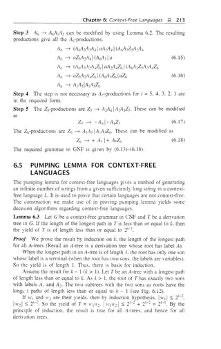
![214 ~ Theory ofComputer Science
A
Fig. 6.12 Tree T with subtrees T1 and Tz.
Theorem 6.10 (Pumping lemma for context-free languages). Let L be a
context-free language. Then we can find a natural number n such that:
(i) Every Z E L with Iz I ~ n can be written as U1'WX)' for some strings
Lt, v, W, x, y.
(ii) l1'xl ~ 1.
(iii) I1'WX I :s; n.
(iv) ll1'k~n):y E L for all k ~ O.
Proof By Corollary 1 of Theorem 6.6, we can decide whether or not A E L.
When A E L, we consider L - {A} and construct a grammar G = (11,,,,, L, P, S)
in CNF generating L - {A} (when A ~ L, we construct Gin CNF generating
L).
Let IVvI = m and n = 21/l. To prove that n is the required number, we
start
with;, E L, IzI ~ 2/ll, and construct a derivation tree T (parse tree) of z. If
the length of a longest path in T is at most m, by Lemma 6.3, Iz I :s; 2111
-] (since
z is the yield of T). But IzI ~ 21/l > 2"-]. So T has a path, say r. of length
greater than or equal to m + 1. r has at least m + 2 vertices and only the last
vertex is a leaf. Thus in r all the labels except the last one are variables. As
Iv'v I = m. some label is repeated.
We choose a repeated label as follows: We start with the leaf of rand
travel along r upwards. We stop when some label, say B. is repeated. (Among
several repeated labels, B is the first.) Let v] and 1'2 be the vertices with label
B, VI being nearer the root. In r. the portion of the path from v] to the leaf has
only one labeL namely B, which is repeated, and so its length is at most m + 1.
Let T) and T2 be the subtrees with vj, 1'2 as roots and z), W as yields,
respectively. As r is a longest path in T, the portion of r from v) to the leaf
is a longest path in T] and of length at most m + 1. By Lemma 6.3, Iz] I:s; 2m
(since z] is the yield of T]).
For better understanding, we illustrate the construction for the grammar
whose productions are S ~ AB, A ~ aB Ia, B ~ bA Ib, as in Fig. 6.13. In
the figure,
r= S ~ A ~ B ~ A ~ B ~ b
z = ababb. ;,) = bab, w = b
V = ba. x = A, II = a, y = b](https://image.slidesharecdn.com/automata-150510143406-lva1-app6891/85/Automata-227-320.jpg)
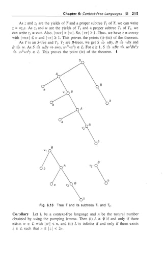


![Chapter 6: Context-Free Languages ,i;l, 219
So ababbab E L(G).
S ~ A2aAbA2 (as in the derivation of the first string)
~ aaaabaa
S ~ A2
aAbA2
~ bbabbbb
So ababbab, aaaabaa, bbabbbb are in L(G).
(c) S ~ ASA. If B ~ 11', then 11' starts with a and ends in b or vice versa
and I,v I 2': 3. If aaa is in L(G), then the first two steps in the
derivation of aaa should be S ~ ASA ~ ABA or S ~ aBa. The
length of the terminal string thus derived is of length 5 or more.
Hence aaa 9!: L(G). A similar argument shows that bbb 9!: L(G).
S ~ B ~ acb ~ aAb ~ abb. So abb E L(G)
(d) False. since the single-step derivations starting with C can only be
C ~ ACA or C ~ A.
(e) C ~ ACA ~ AAA ~ bab. True
(f) Let 11' = abab. If C ~ 11', then C ~ ACA ~ 11' or C ~ A ~ 11'.
In the first case 111'1 =3, 5. 7..... As 111'1 =4. and A ~ 11' if and
only if 11' =a or b, the second case does not arise. Hence (f) is false.
(g) C ~ ACA ~ AAA. Hence C ~ AAA is true.
(h) A 9!: L(G).
EXAMPLE 6.21
If G consists of the productions S ~ aSa IbSb I aSb I bSa I A, show that L(G)
is a regular set.
Solution
First of all, we show that L(G) consists of the set L of all strings over {a, b}.
of even length. It is easy to see that L(G) I: L. Consider a string 11' of even
length. Then, 11' =aja2 ... a2n-Ia2n where each ai is either a or b. Hence
S ~ a1Sa2n ~ aja2Sa211_ja2n ~ aja2 ... al1San+j ... a2n ~ a1a2 ... a21]'
Hence L I: L(G).
Next we prove that L = L(G1) for some regular grammar Gj • Define
G1 = ({S, Sl' S2' S3' S4}. {a, b}. P, S) where P consists of S ~ aSj, Sl ~ as,
S ~ aS2, S2 ~ bS, S ~ bS3• S3 ~ bS, S ~ bS4• S4 ~ as, S ~ A.
Then S :b aja2S where a1 = a or band a2 = a or b. It is easy to see that
L(G1) = L. As Gj is regular, L(G) =L(Gj ) is a regular set.
EXAMPLE 6.22
Reduce the following grammar to CNF:
S ~ ASA IbA. A ~ BIS, B~c](https://image.slidesharecdn.com/automata-150510143406-lva1-app6891/85/Automata-232-320.jpg)
![Chapter 6: Context-Free Languages ~ 221
any production of G. Show that there exists an equivalent grammar GI m
CNF, which has at most (k - l)IPI + ILl productions.
Solution
In step 2 (Theorem 6.8). a production of the form A ~ XIX::: ... Xil is
replaced by A ~ Yj Y:::, ...• Yll where Yi = Xi if Xi E VN and Yi is a new
variable if Xi E I.. We also add productions of the form Yi ~ Xi whenever
Xi E I. As there are II Iterminals, we have a maximum of II. Iproductions of
the form Yi ~ Xi to be added to the new grammar. In step 3 (Theorem 6.8),
A ~ AjA::: ... An is replaced by n - 1 productions, A ~ AIDj. D] ~ A2D:::
... DIl
_::: ~ An_jAil' Note that n S k. So the total number of new productions
obtained in step 3, is at most (k - 1) 1P I. Thus the total number of productions
in CNF is at most (k - l)IPI + II. I·
Example 6.24
Reduce the following CPG to GNF:
S ~ ABbla, A ~ aaA. B ~ hAb
Solution
The valid productions for a grammar in GNF are A ~ a (X, where a E L,
0; E V~v.
So, S ~ ABb can be replaced by S ~ ABC, C ~ b.
A ~ aaA can be replaced by A ~ aDA. D ~ a.
B ~ hAb can be replaced by B ~ hAC. C ~ b.
So the revised productions are:
S ~ ABC I a, A ~ aDA, B ~ hAC. C ~ b. D ~ a.
Name S, A, B, C, D as A b A:::, A3, A4• As.
Now we proceed to step 2.
Step 2 G1 = ({AI, A:::, A3, A4, As}, {a, b}, PI, AI) where PI consists of
Al ~ A:::Afi41 a, A::: ~ aAsA:::, A3 ~ bA:::A4, A4 ~ b. As ~ a
The only production to be modified using step 4 (refer to Theorem 6.9)
is AI ~ A:::Afi4'
Replace Al ~ A:::Afi4 by Al ~ aAsA:::Afi4'
The required grammar in Gr-..Tf is
G2 = ({A b A2. ,13, A~, As}, {a, b}, Pb AI) where P2 consists of
AI ~ aAsAfi41 a
A2 ~ aAsA2
A3 ~ bA2A4, A4 ~ b, As ~ a](https://image.slidesharecdn.com/automata-150510143406-lva1-app6891/85/Automata-234-320.jpg)
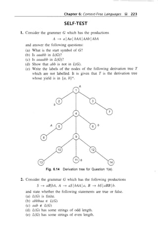


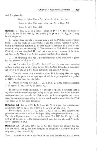
![230 !ii Theory of Computer Science
For a finite automaton. the working can be desclibed in terms of change
of states. In the case of pda, because of its additional structure, namely PDS,
the working can be described in terms of change of IDs. So we have the
following definition:
Definition 7.4 Let A be a pda. A move relation, denoted by r-' between IDs
is defined as
(q. a1 a2 ... (In' Z1Z2 ... Zm) r- (q', {l2a3 ... (1m ,8Z2 ... Zm)
if o(q, (II' ZI) contains (q', {3).
Note: The move relation
(q, a1a2 ... ({'" Z1Z2 ... Z",) r- (q', {l2{13 ... all' {3Z2 Zm)
can be described as follows: The pda in state q with Z1Z2 Zm in PDS
(ZI is at the top) reads the input symbol al' When (q', j3) E o(q, {lj, Zd. the
pda moves to a state q' and writes {3 on the top of Z2 . " Zm. After this
transition. the input string to be processed is {l2a3 ... all"
If f3 = Y1 Y2 Y~. then Fig. 7.2 illustrates the move relation.
L--_la1Ia2j lanl
b;j ~I . I
I 2m I
Fig. 7.2 An illustration of the move relation.
Remark As r- defines a relation in the set of all IDs of a pda, we can define
the reflexive-transitive closure r- which represents a definite sequence of n
moves, where II is any non-negative integer.
If (q, x. a) r- (q', y. j3) represents n moves. we write (q, x. ex) P-
(q'. }'. (3). In particular, (q, x. a) ~ (q, x, a). Also, (C], x. a) r- (q', y, j3)
can be split as
(q, x, a) r- (Q1' Xl. 0'1) r- (Q2. x.:> cee) r- ... r- (q', y. P)
Note: When we deal vith more than one pda, we also specify the pda while
desclibing the move relation. For example, a move relation in A is denoted
bv I •
-~](https://image.slidesharecdn.com/automata-150510143406-lva1-app6891/85/Automata-243-320.jpg)
![Chapter 7: Pushdown Automata J;! 231
The next two results are properties of the relation ~ and are frequently
used in constructions and proofs.
Result 1 If
(7.1)
then for every y E r*.
(qj, xy. a) ~ (q~, y, {3) (7.2)
Conversely, if (Cjj. A}'. a) ~ (q~. Y. 13) for some :v E r*, then (qj. x. a) ~
(q~. A, /3).
Proof The result can be easily understood once we refer to Fig. 7.2.
providing an illustration of the move relation.
If the pda is in state ql with a in PDS. and the moves given by (7.1) are
effected by processing the string x. the pda moves to state q~ with 13 in PDS.
The same transition is effected by starting with the input string xy and
processing only x. In this case, y remains to be processed and hence we
get (7.2).
We can prove the converse part i.e. (7.2) implies (7.1) in a similar way.
Result 2 If
then for every 13 E f*.
(q. x. a) ~ (q'. A, y) (7.3)
(7.4)(q. x. a/3) ~ (q', A, yf3)
Proof The sequence of moves given by (7.3) can be split as
(q, x. a) f- (qt- Xl' aj) f- (q2. X2· a2) f- ... f- (q'. A, y)
Consider (qi' Xi. ail f- (qi+l' xi+1' ai+l)' Let ai =ZIZ~ ... ZIII·As a result
of this move. Zj is erased and some string is placed above Z~ . , . ZiJl' So.
Z2 .,. ZIII is not affected. If we have 13 below Z2 ... ZI'" then also
Z2 ... Zmf3 is not affected. So we obtain (qj, Xj, ai/3) f- (qi+l' Xj+1' aj+i/3)·
Therefore. we get a sequence of moves .
(q. x. af3) f- (qj. XI. ajf3) f- ... f- (C]', A. yf3)
I.e.
(q, x. af3) ~ (q'. A. yf3)
Note: In general. (7.4) need not imply (7.3). Consider. for instance,
A = ({qo}, {a, b}, {Zo}, 8, qo· Zo, 0)
where
8(qo· a. Zo) ={(qo· A)}. 8(qo. b. Zo) = {(qo. ZoZo)}
(qQ. aab. ZoZoZoZo)
f- (qo, abo ZoZeJZo)
f- (qo. b. ZoZo)
f- (qo· A. ZoZoZo)](https://image.slidesharecdn.com/automata-150510143406-lva1-app6891/85/Automata-244-320.jpg)

![Chapter 7: Pushdown Automata J;;;! 233
Proceeding in a similar way, we can show that
(qo, wew
T
. 4J) p:- (qt. A, Zo) for all >t' E {a, b} *
Suppose an initial configuration is (qo, abehb, Zo). Then, we have
(qo. abebb. Zo) r- (qo. bebb, aZo) by Rule (7.5)
r- (qo, ebb, baZo) by Rule (7.6)
r- (q]. bb. baZo) by Rule (7.8)
r- (q], b. aZo) by Rule (7,9)
Once the pda is in ill (q!> b, aZo), it has to haIt as /S(q], b. a) = 0. Hence,
we have
(qo, abebb. Zo) p:- (q], b, aZo)
As /S(LJa. e. 4J) = 0, the pda cannot make any transition if it starts with an
ill of the form (qo. ew. 4J).
Note: In Example 7.2. each /S(q, a. Zl is either empty or consists of a single
element. So for making transitions. the pda has only one choice and the
behaviour is deterministic.
In general. a deterministic pda can be defined as follows:
Definition 7.5 A pda A = (Q. L r. /5. qo. Zoo F) is deterministic if
(i) /S(q. a, Z) is either empty or a singleton. and (ii) /S(q. A. Z) 1= 0 implies
/S(q, a, Z) = 0 for each a E L.
Consider the pda given in Example 7.2. /S(q. a. Z) given by Rules
(7.5)-(7.10) are singletons, Also. /S(q], a. Zo) = 0 and /S(q]. a, Zo) = 0 for
all a E L, So the pda given in Example 7.2 is deterministic.
7.2 ACCEPTANCE BY pda
A pda has final states like a nondeterministic finite automaton and has also the
additional structure. namely PDS, So we can define acceptance of input strings
by pda in terms of final states or in terms of PDS.
DefInition 7.6 Let A = CQ, L, r. /S. qo, 20, F) be a pda. The set accepted
by pda by final state is defined by
T(A) = {>t' E L*I(qo. w. Zo) ~ (ql' A. cr.) for some qf E F and cr. E i*}
EXAMPLE 7.3
Construct a pda A accepting L = {wewT
i>t' E {a. b} *} by final state.](https://image.slidesharecdn.com/automata-150510143406-lva1-app6891/85/Automata-246-320.jpg)
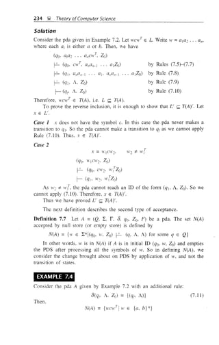
![Chapter 7: Pushdown Automata l;l 235
Solution
From the construction of A, we see that the Rules (7.5)-(7.10) cannot erase
Zoo We make a provision for erasing Zo from PDS by Rule (7.11). By
Example 7.2, wcwT
E T(A) if and only if the pda reaches the ill (qj' A, Zo)'
By (7.11), PDS can be emptied by A-moves if and only if the pda reaches the
ill (qr, A, Zo). Hence.
N(A) = {lvcwT
Iw E {a, b} *}
In the next theorem we prove that the set accepted by a pda A by null store
is accepted by some pda B by final state.
Theorem 7.1 If A = (Q, L, r, 0, qo, Zo, F) is a pda accepting L by empty
store. we can find a pr1
:t
B = (Q', L, r', os, q'o, Zo, F')
which accepts L by final state, i.e. L = N(A) = T(B).
Proof B is constructed in such a way that (i) by the initial move of B, it
reaches an initial ill of A. (ii) by the final move of B, it reaches its final state,
and (iii) all intermediate moves of B are as in A.
Let us define B as follows:
where
q'o is a new state (not in Q).
F' = {qj}' with qf as a new state (not in Q),
Q' =Q u {q'o, qj},
Z'o is a new start symbol for PDS of B.
r' = r u {Zo}, and
0B is given by the rules R b R2, R3
with
R( 0s(q'o. A, Z'o) = {(qo, ZoZ'o)}.
R2: OB(q, a, Z) = O(q, Cl, Z) for all (q, a, Z) in Q x (L u {A}) x r
R3: 0B(q, A, Z'o) = {(qf' A)} for all q E Q.
By Rj, the pda B moves from an initial ill of B to an initial ill of A.
R j gives a A-move. As a result of Rj, B moves to the initial state of A with
the start symbol Zo on the top of PDS.
R2 is used to simulate A. Once B reaches an initial ill of A. R2 can be used
to simulate moves of A. We can repeatedly apply R2 until Z'o is pushed to the
top ('f PDS. As Z'o is a new pushdown symbol, we have to use R3.
R3 gives a A-move. Using R3• B moves to the new (final) state qf erasing
Z'o in PDS.
Thus the behaviour of B and A are similar except for the A-moves given
by R] and R3. Also, W E T(B) if and only if Breaches qf, i.e. if and only](https://image.slidesharecdn.com/automata-150510143406-lva1-app6891/85/Automata-248-320.jpg)
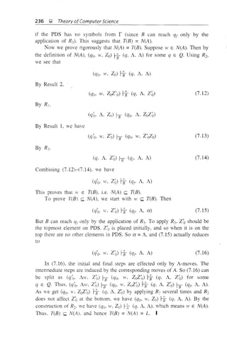
![Chapter 7: Pushdown Automata J;L 237
Note: From the construction of B. it is easy to see that B is deterministic if
and only if A is deterministic.
EXAMPLE 7.5
Consider the pda A given in Example 7.1 (Take F = 0). Determine N(A).
Also construct a pda B such that T(B) =N(A).
Solution
where 8 is given by
R j : 8(qo, a. Zo) = {(qo, aZo)}
R< 8(qo. a, a) = {(qo, aa)}
R3: 8(qo, b. a) = {(qj, A)}
R+: 8(qj. b, a) = {(qj. A)}
Rs: 8(qj, 1. Zo) = {(qj. A)}
Rj is used to store a in PDS if it is the first symbol of an input string.
R: can be used repeatedly to store a" in PDS. When b is encountered for the
first time in the input string. a is erased (in PDS) using R3. Also, the pda
makes a transition to state qj. After processing the entire input string, if Zo
remains in PDS, it can be erased using the null move given by Rs. So, if
],V = d'b", then we have
(qo. d'Y'. Zo) pc- (qo· b", a"Zo) by applying Rj and R:
pc- (q j. A. Zo) by applying R3 and R4
r- (qt, A, A) by applying Rs
Therefore. a"b" E N(A).
If H' E N(A). then (qo. w, Zo) pc- (ql, 1, A). (Note that the PDS can be
empty only when A is in state qj') Also, ],V should start with a. Otherwise, we
cannot make any move. We store the symbol a in PDS if the current input
symbol is a and the topmost symbol in PDS is a or Zoo On seeing the input
symbol b, the pda erases the symbol a in PDS. The pda enters the ill (qj, A, A)
only by the application of Rs. The pda can reach the ill (qj, A, Zo) only
by erasing the a's in pda. This is possible only when the number of b's is
equal to number of a's, and so 1" = a"Yl. Thus. we have proved that
N(A) = {a"b"ln;:: l}.
~ow let
B = (Q'. {a, b}. r', 8B• q'o. Z'o. F')
where
r' = {a. b. Z'o}](https://image.slidesharecdn.com/automata-150510143406-lva1-app6891/85/Automata-250-320.jpg)
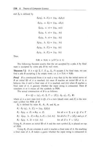
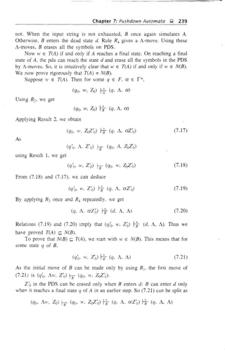
![240 ~ Theory ofComputer Science
for some q E F and ex E P'. But (qo. w, ZoZ~)) ~ (q, A, exZ'o) can be
obtained only by the application of R2• So the moves involved are those
induced by the moves of A. As Z'o is not a pushdown symbol in A, Z'o lying
at the bottom is not affected by these moves. Hence
(c/o, Aw, Z~)) rt (q. A. ex), q E F
So w E T(A) and N(B) ~ T(A). Thus,
L = N(B) = T(A)
EXAMPLE 7.6
Construct a pda A accepting the set of all strings over {a, b} with equal
number of a's and b·s.
Solution
Let
A =({q), [a. b]. [Zo, a, b], D, q, Zo, 0)
where Dis defined by the following rules:
D(q, a, Zo) = {(q, aZo)} D(q. b, Zo) = {(q, bZo)}
D(q, a. a) = {(q. aa)} D(q, b. b) = {(q, bb)}
D(q. a. b) = {(q. A)} D(q. b, a) = {(q. A)}
D(q. A, Zo) = {(q, A)}
The construction of Dis similar to that of the pda given in Example 7.2.
But here we want to match the number of occurrences of a and b: so, the
construction is simpler. We start by storing a symbol of the input string and
continue storing until the other symbol occurs. If the topmost symbol in PDS
is a and the current input symbol is b. a in PDS is erased. If lV has equal
number of a's and b's, then (q. w. Zo) ~ (q, A, Zo) 1- (q, A, A). So
WE N(A). We can show that N(A) is the given set of strings over {a. b} using
the construction of 0.
7.3 PUSHDOWN AUTOMATA AND CONTEXT-FREE
LANGUAGES
In this section we prove that the sets accepted by pda (by null store or final
state) are precisely the context-free languages.
Theorem 7.3 If L is a context-free language, then we can construct a pda
A accepting L by empty store, i.e. L = N(A).](https://image.slidesharecdn.com/automata-150510143406-lva1-app6891/85/Automata-253-320.jpg)

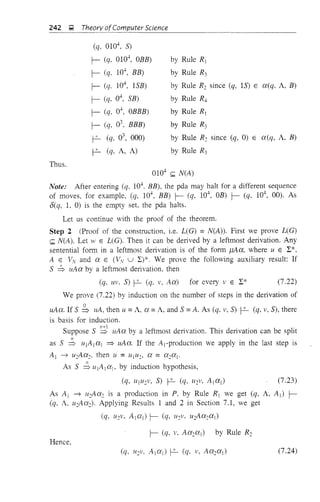
![Chapter 7: Pushdown Automata ~ 243
But U111: = u and a2a1 = ex. So from (7.23) and (7.24), we have
(q, uv, S) P- (q, v, Aa)
Thus (7.22) is true for S ~ uAa. By the principle of induction, (7.22) is true
for any derivation. Now we prove that L(G) k N(A). Let W E L(G). Then,
w can be obtained from a leftmost derivation,
S ~ uAv ~ uu'v =W
From (7.22),
(q, uu'v, S) P- (q, u'v, Av)
As A ~ u' is in P,
(q, u'v, Av) P- (q, z/v. u'v)
By Rule R:.
(q, u'v, u'v) p- (q, A, A)
Therefore,
Next we prove
tV = uu'v E N(A) proving L(G) k N(A)
N(A) k L(G)
Before proving the inclusion, let us prove the following auxiliary result:
S ~ ua if (q. uv, S) P- (q, v, a) (7.25)
We prove (7.25) by the number of moves in (q. uv, S) P- (q, v, a).
o
If (q, uv, S) p1- (q, v, a). then 1I =A, S =a; obviously, S => Aa. Thus
there is basis for induction.
Let us assume (7.25) when the number of moves is n. Assume
l"+l
(q, UV, S) r- (q, v, a) (7.26)
The last move in (7.26) is obtained either from (q, A, A) I- (C], A, a') or
from (q, a, a) I- (q, A, A). In the first case. (7.26) can be split as
(q, uv, S) P- (q, v, Aa:) I- (q, v, ala:) =(q, v, a)
By induction hypothesis, S ~ uAa2, and the last move is induced by
A ~ al' Thus, S ~ uAa: implies a1 a2 =ex. So,
S ~ lIAa: ~ uaJa2 = ua
In the second case. (7.26) can be split as
(q, uv, S) P- (q, av, aa) I- (q, v, a)
Also. 1I = u'a for some u' E L. So. (q, !I'av, S) P- (q, av, aa) implies (by
induction hypothesis) S ~ !I'aa =!la. Thus in both the cases we have shown
that S ~!lex. By the principle of induction, (7.25) is true.](https://image.slidesharecdn.com/automata-150510143406-lva1-app6891/85/Automata-256-320.jpg)
![244 g Theory ofComputer Science
Now, we can prove that if >v E N(A) then W E L(G), As W E N(A),
we have (q, w, S) r- (q, A, A), By taking II =W, V =A, ex =A and applying
(7,25), we get S ::; wA =H', i,e, w E L(G). Thus,
L(G) = N(A)
Theorem 7.4 If A = (Q, L. r, 0, qo. Zoo F) is a pda. then there exists a
context-free grammar G such that L(G) =N(A).
Proof We first give the construction of G and then prove that N(A) = L(G).
Step 1 (Construction of G). We define G = (Vv, L, P, S), where
Vv = {S} u {[q, Z, q'] Iq. q' E Q, Z E l}
i.e. any element of Vv is either the new symbol S acting as the start symbol
for G or an ordered tliple whose first and third elements are states and the
second element is a pushdown symbol.
The productions in P are induced by moves of pda as follows:
R j: S-productions are given by S ~ [qo, Zo, q] for every q in Q.
R< Each move erasing a pushdown symbol given by (q', A) E O(q, a, Z)
induces the production [q, Z, q'] ~ a.
R,,: Each move not erasing a pushdown symbol given by (qlo ZtZ: ... Zm)
E O(q, a, Z) induces many productions of the form
[q, Z, q'l ---7 a[qj. Zj, q:1[q:. Z:, q3] ... [qm' Zm' q']
where each of the states q', q2, .. " qll' can be any state in Q. Each move yields
many productions because of R3• We apply this construction to an example
before proving that L(G) = N(A).
EXAMPLE 7.8
Construct a context-free grammar G which accepts N(A), where
A = ({qo, qd, {a. b}, {Zo° Z}, 0, qo, Zo, 0)
and 0 is given by
O(qo, b, Zo) = {(qo, ZZo)}
O(qo, A, Zo) = {(qo, A)}
O(qo, b. Z) = {(qo, ZZ)}
O(qo, a, Z) = {(qj, Z)}
O(qj. b, Z) = {(qj. A)}
O(qj. a, 20) = {(qo, Zo)}
Solution
Let
G = (Vy. {a. b}, P. S)](https://image.slidesharecdn.com/automata-150510143406-lva1-app6891/85/Automata-257-320.jpg)
![Chapter 7: Pushdown Automata g 245
where Vv consists of S, [qo, Zo, qo], [qo, Zo, qd, [qo· Z. qa], [qo, Z, ql),
[CiI' Zoo qo], [cll, Zoo Cid, [c11. Z, Cio], [qj, Z. qd·
111e productions are
Pi: S -1 [qo, Zo, qe]
Po: S -1 [qo· Zo° qrJ
01 qo. b, Zo) = {(qe. ZZo)} yields
Po: [qo. Zo, qo] -1 b[qo. Z. qo][qo· ZCh qo]
P4: [qo. Zo, Cio] -1 b[Cio· Z, Lll][qj, Zo, qo]
Ps: [qo, Zoo qd -1 b[qo. Z, qa][qo, Zo, CiI]
P6: [c/o, Zo, q] -1 b[qo, Z, qI][c/1, Zo, qI]
o(qo. A. Ze) = {(qo, A)} gives
P7: [qo, Zo, qo] -1 A
o(qo. b. Z) = {(CJo. ZZ)} gives
Pg: [qo· Z. Cla] -1 b[c/o· Z. (/0] [qo, Z. qo]
P9: [cIa· Z. qo] -1 b[qo, Z. qd[Clj· Z, qo]
PIO: [qo· Z. qd -1 b[qo· z. qo][qo, Z. qd
P II : [qe, Z. ql] -1 b[Clo. z. ql][q], Z, LJI]
olqe, a. Z) {(LJI' Z)} yields
PI~: [cia, Z. LJo] -1 a[q], Z. qo]
P13 : [qo. Z. qd -1 a[qj, Z, q]]
6((/]. b. Z) = {(LJl , A)} gives
P14: [ql' Z. qd -1 b
6(ql' a. Zo) = {(qe· Zo)} gives
PIS: [qj, Zo, qo] -1 a[qo, Zo, qo]
P 16: [ell' Zo° ql] -1 a[qij, Zo, ql]
P1-P16 give the productions in P.
Using the techniques given in Chapter 6. we can reduce the number of
variables and productions.
Step 2 Proof of the constmction. i.e. N(A) = L(G).
Before proving that ll(A) = L(G), we note that a variable [q. Z. q'] indicates
t::it for the pda the current state is q and the topmost symbol in PDS is Z In
the course of a delivation. a state q' is chosen in such a way that the PDS is
emptied ultimately. This corresponds to applying R~. (Note that the production
given by R~ replaces a variable by a terminaL)](https://image.slidesharecdn.com/automata-150510143406-lva1-app6891/85/Automata-258-320.jpg)
![246 ~ Theory ofComputer Science
To prove N(A) = L(G), we need an auxiliary result, i.e.
*
[q, Z, q'] =g w
if and only if
(7.27)
(q, W, Z) r-- (q', A, A) (7.28)
We prove the 'if part by induction on the number of steps in (7.28). If
(q, w, Z) r- (q', A, A), then W is either a in I: or a in A. So, we have
(q', A) E 8(q, w, Z)
By R2 we get a production [q, Z, q'] ~ w. So, [q, Z, q'] ~ w. Thus there
is basis for induction. G
Let us assume the result, namely that (7.28) implies (7.27) when the
former has less than k moves. Consider (q, w, Z) t-L (q', A, A). This can be
split as
(7.29)
where W =aw' and a E I: or a =A, depending on the first move.
Consider the second part of (7.29). This means that the PDS has Z1Z2 ...
ZIl1' initially, and on application of w, the PDS is emptied. Each move of pda
can either erase the topmost symbol on the PDS or replace the topmost symbol
by some non-empty string. So several moves may be required for getting on the
top of PDS. Let WI be the prefix of w such that the PDS has Z2Z3 ... Zm after
the application of WI' We can note that the string Z2Z3 ... Zm is not disturbed
while applying WI' Lei Wi be the substring of w such that the PDS has
Zi+I ... Zm on application of Wi' Zi+I ... Zm is not disturbed while applying
Wb W2, .. "' H'i' The changes in PDS are illustrated in Fig. 7.3.
Z1
Z2 (' Z2 Z2
Zi
Zi+1 ?
Z~1?w Empty
bd
store
Zm Zm Zm Zm Zm Zm
'--r----J
w1 w2 wm
Fig. 7.3 Illustration of changes in pushdown store.](https://image.slidesharecdn.com/automata-150510143406-lva1-app6891/85/Automata-259-320.jpg)
![Chapter 7: Pushdown Automata ~ 247
In terms of IDs, we have
(qi, Wi, Z) f-2- (qi+1> A, A) for i = 1, 2, ..., m, qm+l = qt (7.30)
As each move in (7.30) requires less than k steps, by induction hypothesis we
have
(7.31 )
The first part of (7.29) is given by (% ZjZ2 ... ZII/) E /5(q, a, Z). By R3
we get a production
[q. Z, qt] ::S a[qj, Z1> q2][q2, Z2, q3] ... [qll/' Zm. qt]
From (7.31) and (7.32), we get
[q, Z. qt] ::S aWl w2 ... Hill/ = W
(7.32)
By the principle of induction. (7.28) implies (7.27).
We prove the 'only if part by induction on the number of steps in the
derivation of (7.27). Suppose [q, Z. q'] ~ w. Then [q. Z, qt] ~ W is a
production in P. This production is obtained by R2. So W =A or W ELand
(q', A) E /5(q. ,V, Z). This gives the move (q, w, Z) r- (q, A, A). Thus there
is basis for induction.
Assume the result for derivations where th~ number of steps is less than k.
Consider [q, Z. qt] b w. This can be split as
[q. Z. qt] ~ a[qJ. Zl' q2][q2. Z2. q3] ... [qll1' Z"" qt] k;1 W (7.33)
As G is context-free, we can write W =aWjW2 ... w"', where
[qi, Zi, qi+d ~ Wi and qll/+ 1 = qt
C'
By induction hypothesis. we have
for i = 1, 2, ..., m(qi' Wi, Z) f-2- (qi+l' A, A)i
By applying Results 1 and 2, we get
(qi. Wi, ZiZi+l ... ZII/) f-2- (qi+j, A, Zi+l ... Zm)
(7.34)
(Cli' WiWi+] ... WII/' Zi ... Zm) r- (qi+h Wi+l ... H'I/l' Zi+l ... Zm) (7.35)
By combining the moves given by (7.35), we get
(q], W]W2 ... WII/' Zl ... ZII/) f-2- (q', A, A) (7.36)
The first step in (7.33) is induced by (q]. Z]Z2 ... ZII/) E /5(q, a, Z). The
corresponding move is
(q, a, Z) r- (qj, A, ZjZ2 ... ZIl1)
By applying the Result 1, we get
(q, aWl ... Will' Z) r- (qJ. W] .. , WII/' ZI ... ZII;) (7.37)](https://image.slidesharecdn.com/automata-150510143406-lva1-app6891/85/Automata-260-320.jpg)
![(7.38)
248 ~ Theory ofComputer Science
From (7.37) and (7.36). we get (q, tv, Z) pc- (qt, A, A) . By the principle
of induction, (7.27) implies (7.28).
Thus we have proved the auxiliary result. In particular,
[ql), Zo, ql] ::2> 11 iff (ql). 11', ZI) pc- (qt, /, A)
Now 11' E L(G)
iff 5 :b 1'
iff S ~ lqo, ZQ. Q'1 :b tv (for some q' by R)
iff (qQ, W. Zo) pc- (e/, A. A) by the auxiliary result
iff 11' E N(A)
Thus. N(A) = L(G).
Corollary If A is a pda, then there exists a context-free grammar G such that
T(A) = L(G).
Proof By Theorem 7,2 we can find a pda At such that T(A) =N(A'). By
Theorem 7.4 we can construct G such that N(A') =LI G). Thus T(A) =L(G). I
EXAMPLE 7.9
Construct a pda accepting {a"blild' m. 11 :2': I} by null store. Construct the
corresponding context-free grammar accepting the same set.
Solution
The pda A accepting {(/'bll1
ail
m. n :2': I} is defined as follows:
A = ({qQ. qd, {a. b}, {a, ZQ}, O. qo. ZI). 0)
where 0 is defined by
R1: O(ql), a, Zo) = {(qo. aZo) }
R-,: O(qo· a. a) = { (qa. aa)}
R3: O(qo. b. a) = {(q l' a)}
R.:,: 6Cql' b. a) = {(qj, a)}
Rs: 8(ql' a. a) = {(eil· A)}
R6: 8(Q. A. ZoJ = {(ql, A)}
This is a modification of 8 given in Example 7.2.
We start storing a's until a b occurs (Rules R1 and R:J. When the current
input symbol is b. the state changes, but no change in PDS occurs (Rule R.,).
Once all the b' s in the input string are exhausted (using Rule R4). the
remaining a's are erased (Rule Rs). Using R(). ZI) is erased. So,
(ql). ai/bll'a", Zo) pc- (ql- A. Zo) r-(qlo A. A)
This means that a"blil
(/' E N(A). We can show that
N(A) = {d'b/lla" 1m. n :2': I}](https://image.slidesharecdn.com/automata-150510143406-lva1-app6891/85/Automata-261-320.jpg)
![Chapter 7: Pushdown Automata };l, 249
Define G =(V", {a, b}, P. S). where V" consists of
[qo, 20, qo]. [q1' Zo, qo]· [qo, a, qa], [q), a, qo]
[qo· Zo, q1]' [q), Zo, qI1. [qo· a, qd, [qj, a, qd
The productions in P are constructed as follows:
The S-productions are
PI: 5 -+ [qo, Zo, qa],
8(qo, a. Zo) = {(qo, aZo)} induces
P3: [qo, Zo, qo] -+ a[qo, a, qo][qo. Zo, qo]
P4: [qo, Zo, qo] -+ a[q(j, a. q1][q1, Zo, qo]
P5: [qo· Zo, q!l -+ a[qo, a. qo] [qo, Zoo q1J
P6: [qo, Zo, qj] -+ a[qo, a. ql][q], Zoo ql]
8(qo, a. a) = {(qo. aa)} yields
P7: [qo, a, qo] -+ a[c/o. a. qo][qo, a, qo]
Pg: [qo. a, qoJ -+ a[qo, a. q1][qj, a, qo]
P9: [qo, a. ql] -+ a[qo· a, qo][qo, a. qd
PIO: [qo· a, ql] -+ a[qo, a, q!l[ql, a, q!l
PlJ: [qo, a. qo] -+ b[ql' a. qo]
PI:: [qo· a, qd -+ b[({r, a, q1J
b(qj. b, a) = {(qj, a)} yields
p . [qj. a, qoJ -+ b[qj. a, qaJ. 13'
P j4: [q1, a, qd -+ b[qr, a, qd
8(q], a. 0) = {(qj. A)} gIves
Pj5 : [qj, a, qd -+ a
8(q;, A. Zo) = {(ql, A)} yields
P16: [qj, Zo· ql] -+ A
Note: When the number of states is a large number, it is neither necessary
nor advisable to write all the productions. We construct productions involving
those variables appearing in some sentential form. Using the constructions in
Chapter 6, vve can simplify the grammar further.
Theorem 7.5 Tne intersection of a context-free language L and a regular
language R is a context-free language.](https://image.slidesharecdn.com/automata-150510143406-lva1-app6891/85/Automata-262-320.jpg)
![250 Ji,t Theory ofComputer Science
Proof Let L be accepted by a pda A = (QA' L, T, ~'i' qo, Zo, FA) by final
state and R by DFA M = (QM' L, ~'11' Po, FM)·
We define a pda M' accepting L () R by final state in such a way that M'
simulates moves of A on input a in L and changes the state of M using ~w. On
input A, M' simulates A without changing the state of M. Let
M' = (QM X QA> L, r, 0, [Po, qo]. Zo, FM x FA)
where 0 is defined as follows:
o([p, q], a, X) contains ([P', q'], y) when ~"J(P, a) = p' and 0A(q, a, X)
contains (q', y). o([p, q], A, X) contains ([P, q'], y) when 0A(q, A. X)
contains (q', y).
To prove T(M') =L () R we need an auxiliary result, i.e.
(7.39)
if and only if
(7.40)
We prove the 'only if part by induction on i (the number of steps). If
i =0, the proof is trivial (In this case, p =Po, q =qo, w =A and y= Zo). Thus
there is basis for induction. Let us assume that (7.39) implies (7.40) when the
former has i-I steps.
Let ([Po, qo]. ,v'a, Zo) ~ ([P, q], A, y). This can be split into ([Po, qo],
w'a, Zo) ~ ([p', q']. a, f3) fM; ([P, q], A, y), where w =w'a and a is in L
or a = A depending on the last move. By induction hypothesis, we have
(qo, w', Zo) ~ (q'. A, f3) and o'~IP', w') =p'. By definition of 0, ([P', q'],
a, f3) ~ ([P, q], A, y) implies (q', a, f3) ~ (q, A, y) and o,wCp', a) =p.
(Note: p' =p when a =A.) So, o,'i1<Po, w'a) = o!'<IP', a) =p. By combining
the moves of A, we get (qo, w'a, ZQ) ~ (q', a, {3) ~ (q, A, y), i.e. (qo, w,
ZJ) r±- (q, A. y). So the result is true for i steps.
By the principle of induction the 'only if' part is proved.
We prove the 'if' part also by induction on i. It is trivial to see that there
is basis for induction.
Let us assume (7.40) with i-I steps. Assume that (qo, w, ZQ) ~ (q, A, y)
and ~"ho, w') = p. Writing w as w'a and taking oNIPo. w') as p', we get
(qo, }/a, ZQ) ~ (q', a, {3) ~ (q, A, y). So, (qo, w', 20) iT (q', A, {3).
By induction hypothesis, we get ([Po, qo], w', Zo) ~ ([P', q'], A, {3).
Also, 0fw<P', a) = p and (q', a, {3) ~ (q, A, y) implies ([P', q'], a, {3) ~
([p, qJ, A, y).](https://image.slidesharecdn.com/automata-150510143406-lva1-app6891/85/Automata-263-320.jpg)
![Chapter 7: Pushdown Automata !it 251
Combining the moves. we get ([Po· qo], w. Zo) f-:&- ([p, q], A, y).
Thus the result is true for i steps. By the principle of induction, the 'if'
part is proved.
Note: In Chapter 8 we vill prove that the intersection of two context-free
languages need not be context-free (Property 3. Section 8.3).
7.4 PARSING AND PUSHDOWN AUTOMATA
In a natural language, parsing is the process of splitting a sentence into words.
There are two types of parsing, namely the top-down parsing and the bottom-
up parsing. Suppose we want to parse the sentence "Ram ate a mango." If NP,
VP, N. V, ART denote noun predicate, verb predicate. noun. verb and article,
then the top-down parsing can be done as follows:
5 -1 NPVP
-1 Name VP
-1 Ram V NP
-1 Ram ate ART N
-1 Ram ate aN
-1 Ram ate a mango
The bottom-up parsing for the same sentence is
Ram ate a mango -1 Name ate a mango
-1 Name verb a mango
-1 Name V ART N
-1 NP VN P
-1 NP VP
-15
In the case of formal languages. we derive a terminal string in L(G) by
applying the productions of G. If we know that 11' E L* in L(G), then 5 ~ w.
The process of the reconstruction of the derivation of w is called parsing.
Parsing is possible in the case of some context-free languages.
Parsing becomes important in the case of programming languages. If a
statement in a prograffil11ing language is given. only the derivation of the
statement can give the meaning of the statement. (This is termed semantics.)
As mentioned earlier. there are two types of parsing: top-down parsing and
bottom-up parsing.
In top-down parsing. we attempt to construct the derivation (or the
corresponding parse tree) of the input string. starting from the root (with label
51 and ending in the given input string. This is equivalent to finding a leftmost
derivation. On the other hand. in bottom-up parsing we build the derivation
from the given input string to the top (root '.vith label 5).](https://image.slidesharecdn.com/automata-150510143406-lva1-app6891/85/Automata-264-320.jpg)
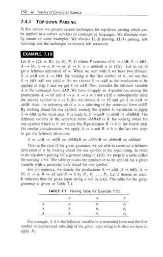

![254 ~ Theory ofComputer Science
In Examples 7.10 and 7.11 for getting a leftmost derivation, one
production among several choices was obtained by look ahead for k symbols.
This kind of nondeterminism cannot be resolved in some grammars even by
looking ahead.
This is the case when a grammar has two A-productions of the form A ~
a{3 and A ~ ay. By a technique called 'left factoring', we resolve this
nondeterminism. Another troublesome phenomenon in a context-free grammar
which creates a problem is called left recursion. A variable A is called left
recursive if there is an A-production of the form A ~ Aa. Such a production
can cause a top-down parser into an infinite loop. Left factoring and technique
for avoiding left recursion are provided in Theorems 7.6 and 7.7.
Theorem 7.6 Let G be a context-free grammar having two A-productions of
the form A ~ a{3 and A ~ ay. If A ~ a{3 and A ~ ay are replaced by
A ~ aA'. A' ~ {3 and A' ~ Y. where A' is a new variable then the resulting
grammar is equivalent to G.
Proof The equivalence can be proved by showing that the effect of applying
A ~ a{3 and A ~ ay in a derivation can be realised by applying A ~ aA',
A' ~ {3 and A' ~ Y and vice versa.
Note: The technique of avoiding nondeterminism using Theorem 7.6 is
called left factoring.
Theorem 7.7 Let G be a context-free grammar. Let the set of all
A-productions be {A ~ Aa1, ..., A ~ Aa,;' A ~ {31' .... A ~ {3m}. Then
the grammar G' obtained by introducing a new vmiable A' and replacing all
A-productions in G by A ~ {31A', ..., A ~ {3I1A', A' ~ a]A', ..., A' ~ a;A'
and A' ~ A is equivalent to G.
Proof Similar to proof of Lemma 6.3.
Theorems 7.6 and 7.7 are useful to construct a top-down parser only for
certain context-free grammars and not for all context-free grammars. We
summarize our discussion as follows:
Construction of Top-Down Parser
Step 1 Eliminate left recursion in G by repeatedly applying Theorem 7.7 to
all left recursive vmiables.
Step 2 Apply Theorem 7.6 to get left factoring wherever necessary.
Step 3 If the resulting grammar is LL(k) for some natural number k, apply
top-down parsing using the techniques explained in Examples 7.10 and 7.11.
EXAMPLE 7.12
Consider the language consisting of all arithmetic expressions involving +, '
( and) over the variables xl and x2. This language is generated by a grammar](https://image.slidesharecdn.com/automata-150510143406-lva1-app6891/85/Automata-267-320.jpg)


![Chapter 7: Pushdown Automata ~ 257
RIO : S(qll' A, B) = (q", as)
R1] S(q". A, B) = (q", b)
R12 Seq, $. 20) = (q, A)
Here R1 changes the initial ill (p, 11', Z) into (q, 11', SZ). R2 and R4 are for
remembering the next symbol. R6-Rll are simulating the productions. R3 and Rs
are for matching the cunent input symbol and the topmost symbol on PDS and
for erasing it (in PDS). Finally. R12 is a move for erasing Z and making the
PDS empty when the last symbol $ of the input string is read.
To get a leftmost derivation for an input string lV, apply the unique
transition given by RJ
to R12• When we apply R6 to R]J, we are using a
cOlTesponding production. By recording these productions we can test whether
]V E L(G) and get a leftmost derivation. The parsing for the input string
abbbab is given m Table 7.4.
The last column of Table 7.4 gives us a leftmost derivation of abbbab. It
is S =} aAB =} abSB =} abbBAB =} abbbAB =} abbbaB =} abbbab.
TABLE 7.4 Top-down Parsing for w of Example 7.13
Step State Unread input Pushdown stack Transition Production
used applied
1 p abbbabS Zo
2 q abbbabS SZo R1
3 qa bbbabS SZo R2
4 qa bbbabS aABZo R6 S ---7 aAB
5 q bbbabS ABZo R3
6 qb bbabS ABZo R4
7 qo bbabS bSBZo Rg A ---7 bS
8 q bbabS SBZo Rs
9 qb babS SBZo R4
10 qb babS bBABZo R7 S ---7 bBA
11 q babS BABZo Rs
12 qb ab$ BABZo R4
13 qb abS bABZo R11 B ---7 b
14 q abS ABZo Rs
15 qa b$ ABZo R2
16 qa b$ aBZo Rg A---7a
17 q b$ BZo R3
18 qb S BZo R4
19 qD $ bZo R1i B ---7 b
q S Zo Rs
21 q A A R12](https://image.slidesharecdn.com/automata-150510143406-lva1-app6891/85/Automata-270-320.jpg)


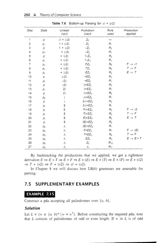
![(7.41)
(7.42)
(7.43)
(7.44)
(7.45)
(7.46)
(7.47)
(7.48)
(7.49)
(7.50)
(7.51)
(7.52)
Chapter 7: Pushdown Automata ~ 261
length, there is a middle symbol which need not be compared with any other
symbol. If w in L is of even length, the rightmost symbol of the first half is
the same as the leftmost symbol of the second half, The key idea of the
construction is to store the symbols in the first half (or the symbols lying to
the left of the middle of the input string) and matching them with the symbols
in the second half (or the symbols to right of the middle of the input string),
If there is no matching. the machine halts.
We define the pda M as follows:
M = ({qo, q], q:c}, {a, b}, {a, b, 2o}, 6, qo, zo, {qJ)
where 6 is defined by
6(qo, G, Zo) = {(qo, aZo), (qj, Zo)}
6(qo, b, Zo) = {(qQ, bZo), (q], Zo)}
6(qo, a. a) = {(qQ, aa), (ql> a)}
6(qo, b, a) = {(qo, ba), (q], a)}
6(qo. a. b) = {(qQ, ab), (qlo b)}
6(qQ' b. b) = {(qQ, bb), (q], b)}
6(qo, A. Zo)= {(q]. Zu)}
6(qo. A, a) = {(q)o n)}
6(qo, A. b) = {(q]. b)}
6(q], n. a)= {(qj. A)}
6(qlo b, b) = {(qlo A)}
6(q], A. Zo) = {(q:c. 2o)}
Obviously, M is a nondeterministic pda. (7.41)~(7.46) give us two
choices. The first choice can be used for storing the input symbol without
changing the state. (7.47)-(7.49) are used for indicating that the first half of
the input string is over: there is change of state in this case. The second choice
of (7.41)-(7.46) is used when w is a palindrome of odd length and the middle
symbol of w is reached: in this case. we ignore the middle symbol and make
no change in PDS. (7.50) and (7.51) are used to match symbols of the input
string (second half) and cancel the symbol in PDS when they match. (7.52)
is used to move to the final state q:c after reaching the bottom of PDS.
We can prove that L is accepted by M by final state. The reader can take
an odd palindrome and an even palindrome and check that the final state q:c
is reached.
EXAMPLE 7.16
Construct a deterministic pda accepting L = {w E {a, b} * Ithe number of a's
in HI equals the number of b's in w} by final state.](https://image.slidesharecdn.com/automata-150510143406-lva1-app6891/85/Automata-274-320.jpg)
![262 iii Theory ofComputer Science
Solution
We define a pda 11 as follows:
lvi = ({Cfo, qd· {a. b}. {a. b. ZoL O. qo, Zo, {qd)
where 0 is defined by
O(q(), a, Zo) = {(qi. Zo)}
O(qo, b. Zo) = {(qo, bZo)}
O(qo, a, b) = {(qo. A)}
O(qo, b, b) = {(qo. bb)}
O(CfI' a, Zo) = {(ql' aZo)}
O(Cfj. h. Zo) = {(qo. aZo)}
O(Cfj, a. a) = {(Cfl, aa)}
O(CfI' b, a) = {(Cfj, A)}
(7.53)
(7.54)
(7.55)
(7.56)
(7.57)
(7.58)
(7.59)
(7.60)
The construction can be explained as follows:
If the pda M is in the final state qj, it means it has seen more a's than
b·s. On seeing the first a. lvi changes state (from qo to ql) «7.53». Afterwards
it stores the a' s in PDS without changing state (7.57) and (7.59». It stores
the initial b in PDS ((7.54» and also the subsequent b's «(7.56». The pda
cancels a in the input string, with the first (topmost) b in PDS «(7.55». If all
b's are matched with stored a's, and M sees the bottom of PDS, M moves
from Cfj to Cfo ((7.58»). The b's in the input string are cancelled on seeing a
in the PDS (7.60»).
Ai is deterministic since 0 is not defined for input A. The reader is advised
to check that Cft is reached on seeing an input string h' in L
EXAMPLE 7.17
Construct a pda M accepting L = {c/hi(J Ii = j or j = k} by final state.
Solution
We define pda M as follows:
I'vi = ({qo. Cfj, ...• Cfd, {a, b, C}. {Z{), X}. 0, Cfo, 20, {Cfj, q3})
where 0 is given by
O(Cfo. A, Zo)= {(Cf], Z{). (Cf2· L{j). (Cf3, Zo)}
o(qj. c. 20)= {(Cf], Zo)}
0(Cf2' a. Zo) = {(Cf2' XZo)}
0(Q2, a. X) = t(Q2, XX)}
O(q2, b, X) = (q)" b. X) = {(Cf)" A)}
O(q),. A. Zo) = {(Cf], Zo)}
(7.61)
(7.62)
(7.63)
(7.64)
(7.65)
(7.66)](https://image.slidesharecdn.com/automata-150510143406-lva1-app6891/85/Automata-275-320.jpg)
![Chapter 7: Pushdown Automata 1; 263
0(q3' a. ZO) = {(q3' Zo)}
0(Q3' b. Zo) = {(q). XZo)}
0«(1). h. X) = {(q). XX)}
O(q). c, X) = O(qc,. c. X) = {(qc" A)}
o(C]c" A. Zo) = {«(/3. A)}
(7.67)
(7.68)
(7.69)
(7.70)
(7.71)
The states qb q:. C]~ stand for aObOck, dbick, dbici respectively where
i > 0, j ;:: O. k ;:: O. (7.61) indicates the initial guess. The three choices
correspond to the three cases.
(q(i. c'. 20) = (qo. Ac
k
• Zo) ~ (qlo c'. Zo) 1- (q], A, Zo)
by (7.61) and (7.62). As ql is a final state. ck
E TUvf).
The pda in state q: will not change state and stores a's in the input string
as X's in PDS «(7.63) and (7,64). On seeing the first b after many a·s. M
changes its state to qJ, and cancels X in PDS for subsequent b's «7.64)). If
it reaches the bottom of PDS. M goes back to ql. which is an accepting state
«(7.76)). So Iv! accepts dbi
• It continuous to be in state q! on seeing c's
subsequently «7.62). So. Ai accepts a'bic'.
For dealing with aibici. Ai makes the initial guess using (7.61) and reaches
state qo. It simply reads a's without changing state or PDS «7.67».
!vI subsequently replaces b with X and changes to state q). Afterwards M
goes on changing b's to Xs «7.69). On seeing a c, !vI changes state.
Subsequent c's are matched with X's (which correspond to b's read earlier)
and X's in PDS are cancelled. On reaching the bottom of PDS, M reaches q3.
a final state «7.71)).
Thus. aOhOck
• (/l/ck
, aibici
E TUYf) for i > O. j ;:: O. k ;:: O. Hence.
T(!vf) = L.
EXAMPLE 7.18
Convert the graJ1lJ11ar 5 -+ aSb! A. A -+ bSa I5 IA to a pda that accepts the
same language by empty stack.
Solution
We construct a pda A as
A = ({q}. {a. b}. {So A. a. b}. o. q, 5.0)
where 0 is defined by the following rules
o(q. A. 5) = {(q. aSb). (q. A)}
o(q. A. A) = {(q, bSA). (q. S). (q. A)}
O(q. a. a) = {(q, A)}
o(q. b. b) = {(C]. A)}
and A is the required pda.](https://image.slidesharecdn.com/automata-150510143406-lva1-app6891/85/Automata-276-320.jpg)

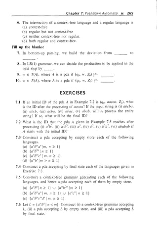


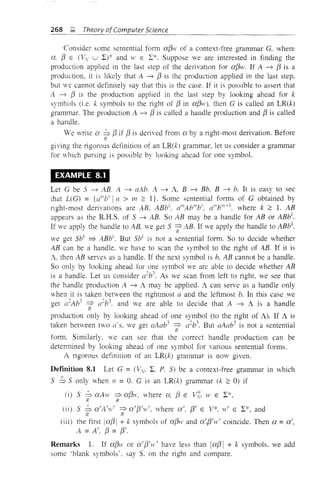
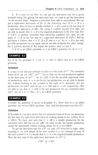
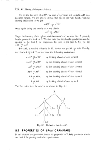
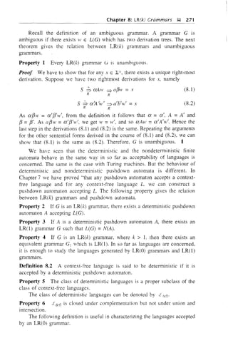
![272 ];i Theory ofComputer Science
~~~--~~~~~~~~~~--~~~
Defmition 8.3 A context-free language has prefix property if no proper
prefix of strings of L belongs to L.
Property 7 A context-free language is generated by an LR{O) grammar if
and only if it is accepted by a deterministic pushdown automaton and has
prefix property.
Property 8 There is an algorithm to decide whether a given context-free
grammar is LR(k) for a given natural number k.
8.3 CLOSURE PROPERTIES OF LANGUAGES
'vVe discussed closure properties under union, concatenation, and so on in
Chapter 4. In this section we will discuss closure properties under intersection,
complementation, etc. Recall that are the families of type 0
languages, context-sensitive languages. context-free languages and regular
languages, respectively.
Property 1 Each of the classes , i fl is closed under union,
concatenation. closure and transpose operations (Theorems 4.5-4.7).
Property 2 is closed under intersection and complementation (Theorems
5.7 and 5.8).
Property 3 ten is not closed under intersection and complementation.
We establish property 3 by a counter-example. We have already seen that
L1 = {a"bile" In 2 1. i 2 O} and L~ = {c/b"e" In 2 1, j 2 O} are context-free
languages (Examples 4.8 and 4.9). L) ( I~ = {d'H'd'ln 2 I}. In Example 6.18.
we have shown that {a"blle"! n 2 I} is not context-free. Thus. is not
closed under intersection.
Using DeMorgan's law. we can write I) ( I~ =(LI U L'2),. We have
proved in Chapter 4 that is closed under union. If were closed under
complementation. then L) (i L~ turns out to be context-free which is not true.
Hence. is not closed under complementation.
8.4 SUPPLEMENTARY EXAMPLES
EXAMPLE 8.4
Show that the grammar 5 ---+ aAc, A ---+ Abb I b is an LR(O) grammar.
Solution
It is easy to see that L(G) ={ab2
"+lc In 2 O}. The sentential forms of G are
aAc. aAb2
"c, ab~l1+ic. We consider the last production applied in the derivation
of ab~I1+1c. As aAc. Abb and b are the possible right-hand sides of productions,](https://image.slidesharecdn.com/automata-150510143406-lva1-app6891/85/Automata-285-320.jpg)
![Chapter 8: LR(k) Grammars ~ 273
only A --+ b can be the last production in the rightmost derivation of aPIl+lc.
(We do not have (lAc and Abb as substrings of ab2n
+] c). Similarly the last
productions for aAc and aAb21l
c are 5 --+ aAc and A --+ Abb respectively.
Hence G is an LR(O) grammar.
EXAMPLE 8.5
Show that S --+ aAb, A --+ cAc I c is not LR(k) for any natural number k.
Solution
It is easy to see that
L(G) = {ac2n
+
1
b 111 2': O}
Consider aeccb E L(G). The last production is A --+ c. But we can apply this
handle only by knowing the entire string. Tnis can be applied to the middle c
but this is knOvn only after looking at two symbols beyond the c which
replaces A. Continuing this argument, we can decide the handle of ac
21l
+
1
b by
only looking at n + 1 symbols beyond the c which replaces A. So it is not
LR(k) for any k.
EXAMPLE 8.6
Give an example of a language which can be generated by an LR(k) gram..'11ar
for some k and also by a grammar that is not LR(k) for any k.
Solution
Consider {ac21l
+1
b In :::: O}. This is generated by the grammar 5 --+ aAb.
A --+ cAc Ic which is not LR(k) for any k.
This language can also be generated by the grammar S --+ aAb,
A --+ Acc Ic. This is LR(O). (This grammar is similar to the grammar in
Example 8A.)
SELF-TEST
Choose the correct answer to Questions 1-5:
1. An LR(k) grammar has to be
(a) a type 0 grammar
(b) a type 1 grammar
(c) a type 2 grammar
(d) none of these.
~ An LR(k) gram..'11ar is
(a) ahvays unambiguous
(b) always ambiguous
(c) need not be unambiguous
(d) none of these.](https://image.slidesharecdn.com/automata-150510143406-lva1-app6891/85/Automata-286-320.jpg)
![274 g, Theory ofComputer Science
3. A handle is
(a) a string of variables and terminals
(b) a string of variables
(c) a string of terminals
(d) a production.
4. The automaton corresponding to an LR(k) grammar is
(a) a deterministic finite automaton
(b) a nondeterministic finite automaton
(c) a deterministic PDA
(d) a nondeterministic PDA.
5. J:dcfl is closed under
(a) union
(b) complementation
(c) intersection
(d) none of these.
EXERCISES
8.1 Show that the grammar 5 ~ aAb. A ~ aAb I a is an LR(l) or is it an
LR(O)?
8.2 Show that the grammar 5 ~ OA2, A ~ L4.1, A ~ 1 is not an LR(O).
8.3 Is 5 ~ AB, 5 ~ aA, A ~ aA, A ~ a, B ~ a an LR(k) for some k?
8.4 Show that {alll
bll1
c" IIn, 11 2': I} u {alll
b"cl1
IIn, 11 2': 1} cannot be generated
by an LR(k) grammar for any k.
8.5 Are the following statements true? (a) If G is unambiguous, it is LR(k)
for some k. (b) If G is unambiguous. it is LR(k) for every k. Justify your
answer.
8.6 Is 5 ~ C ID, C ~ aC Ib, D ~ aD Ian LR(O)?
8.7 For a production A ~ f3 of a context-free grammar G and w in L*$k
($ is a symbol not in Vv U L), define RkC'rv) to be the set of all strings
of the form af3~v such that A ~ f3 is a handle for af3ww' for some w'
in L* $* and 5$ :b aA,nv' => af3'vw'. (In other words, a string af3w is
R R
in Rk(w) if we get a penultimate step of a rightmost derivation of af3ww'
for some w'.) Show that Rk(w) is a regular set.
[Hint: Define G' = (V'v, v.v U L, p', 5'), where
Vv= {[A, w] IA E VN, WE p$k and Iwi = k}
5' = [5, $k]](https://image.slidesharecdn.com/automata-150510143406-lva1-app6891/85/Automata-287-320.jpg)
![Chapter 8: LR(k) Grammars ~ 275
Also show that each production in P induces a production in p' in the
following manner:
(a) If A ~ x is in P, where x E l:*, then [A w] ~ XH' is included in
p'.
(b) If A ~ XIX~ ... XII/ is in P, Xi E Vty, Xi+ l ... XII/H' ~ w'w" for
some w', w" in l:*$* with Iw/l = k, then [A lV] ~ BI ••. Bi-1
[Bi, H"] is included in V
As the productions in p' have either a terminal string or a terminal string
followed by a vmiable on R.H.S., G' can be reduced to an equivalent
regular grammar. Use the principle of induction to show that
[5, $k] ~ [A, w] if and only if for some w'S$k '? aAww
l
This will establish L(G
/
) =Rk(w).
8.8 Prove that a context-free grammar G is an LR(k) if and only if the
follOving holds: A string y in Rk(v,') corresponding to a production
Al ~ 131 is a substring of some element 8 in Rk(W
/
) corresponding to a
production A~ ~ f3~ implies y = 8. Al = A~, 131 = 132'
[Hint: The proof follows from the definition of LR(k) grammars.]
8.9 Prove Property 2 of Section 8.2.
Solution We give an outline of the construction of the required dpda
A A accepts a string w if S$k remains in the stack after the processing
of w. For this purpose. A has to simulate the reverse derivation of w.
This is achieved by finding suitable handles. Rk(w)'s are defined
precisely for this purpose (refer to Exercise 8.7). As Rk(w)'s are regular.
there exist deterministic finite automata Mk(w) corresponding to Rk(w).
For our deterministic pda A to contain the information regarding the
finite automata. the pushdown store of A is required to have an additional
track. In the first track. symbols from Vv u l: are written or erased. In the
additional track, the information regarding Mk(w)'s is stored in the fOlm
of maps. The map Na gives the states of finite automata lvh(w) after the
processing of a string a for all productions in G and strings w in l:*$*
of length k. The existence of a suitable handle is indicated by a final state
of Mk(w) (in the second track).
We can describe the way A acts as follows: A is capable of reading
k + 1 symbols on PDS, where 1 is the length of the longest R.H.S. of
productions of G. (This can be achieved by modifying the finite control.)
A reads the top m symbols on track 1 for some m ~ k + l. The second track
is suitably manipulated. For example. if Xl ... Xm is in track 1, then
track 2 stores the maps NYINxIX2 ... Ny! .. XII1' If a suitable handle is
found, then a sentential form is obtained by replacing the R.H.S. of the](https://image.slidesharecdn.com/automata-150510143406-lva1-app6891/85/Automata-288-320.jpg)


![280 J;;i, Theory of Computer Science
Left sequence
I 8482 •
Right sequence
Present Symbol under
state RIW head
Fig. 9.3 Representation of 10.
Notes: (1) For constructing the ID, we simply insert the current state in the
input string to the left of the symbol under the RIW head.
(2) We observe that the blank symbol may occur as part of the left or right
substring.
Moves in a TM
As in the case of pushdown automata, 8(q, x) induces a change in ID of the
Turing machine. We call this change in ID a move.
Suppose 8(q, Xj) =(P, y, L). The input string to be processed is X1X2 ... Xn,
and the present symbol under the RIW head is Xi' So the ID before processing
Xi is
After processing Xi, the resulting ID is
This change of ID is represented by
If i = 1, the resulting ID is p Y X2 X3 ••. XI/'
If 8(q, xJ = (p, y, R), then the change of ID is represented by
Xj X2'" 'Yi-1q xi'" .In r- X j X 2'" Xi-lypXi+l'" x"
If i = 11, the resulting ID is XjX2 ... Xn-l Y P b.
We can denote an ill by Ij for some j. Ij r-1k defines a relation among IDs.
So the symbol f2- denotes the reflexive-transitive closure of the relation r-'
In particular, Ij f2- Ij . Also, if I] f2- In' then we can split this as II r- 12 r-
Io r- ... r- I" for some IDs, 12, ... , 1,,-1'
Note: The description of moves by IDs is very much useful to represent the
processing of input strings.
9.2.2 REPRESENTATION BY TRANSITION TABLE
We give the definition of 8 in the form of a table called the transition table. If
8(q, a) = (y, a. (3). we write a(3yunder the a-column and in the q-row. So if](https://image.slidesharecdn.com/automata-150510143406-lva1-app6891/85/Automata-293-320.jpg)


![Chapter 9: Turing Machines and Linear Bounded Automata ~ 283
The change brought about by processing the symbol 0 can be represented as
-t J-
bOOllb (O.x.R) > bxOllb
qj q2
~b
Rrw head
Fig. 9.5 TM processing 0011.
The entire computation sequence reads as follows:
J- J- J-
bOOllb
(O.x.R!
bxOllb
(O.O.RI
bxOllb) ~
ql q2 q2
J- J- J-
(l.,'.LI ) bxOylb (O.O.L) ) bxOylb (x.x.R)
bxOvlb)
qo, q4 ql
J-
IO.x.R) 'b b--~) xxvI
q2
J-('.'.R)
,. ) bxxylb
q2
J-(1.'.L)
, ) bxxyyb
qj
(".,LI J- (x..t.R) b J, (".".R) J,
" >bxxyyb ) xxyyb " ) bxxyyb
qo, qs qs
(,. ,.R) J, (b.b.R) J,
" ) bxxyyb ) bxxyybb
qs q6
9.3 LANGUAGE ACCEPTABILITY BY TURING
MACHINES
I F't us consider the Turing machine M = (Q. '2:, 1. (5, qo, b. F). A string w in
'2:* is said to be accepted by M if qoVl' r- (XIP(X2 for some P E F and (x], (X:c
E r*.
M does not accept VI' if the machine M either halts in a nonaccepting state
or does not halt.](https://image.slidesharecdn.com/automata-150510143406-lva1-app6891/85/Automata-296-320.jpg)
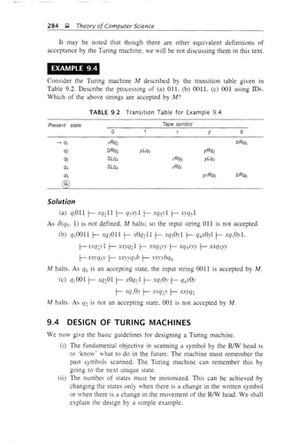
![Chapter 9: Turing Machines and Linear Bounded Automata g 285
EXAMPLE 9.5
Design a TUling machine to recognize all stlings consisting of an even number
of 1's.
Solution
The construction is made by defining moves in the following manner:
(a) ql is the initial state. M enters the state q2 on scanning 1 and writes b.
(b) If M is in state q2 and scans 1, it enters q, and writes b.
(c) q] is the only accepting state.
So M accepts a stJing if it exhausts all the input symbols and finally is in
state qj. Symbolically,
M = ({qj, q2}, {I. b}, {l, b}, 8, q, b. {qd)
"here 8 is defined by Table 9.3.
TABLE 9.3 Transition Table for Example 9.5
Present state
Let us obtain the computation sequence of 11. Thus, q j ll f- bq21 f- bbql'
As ql is an accepting state. 11 is accepted. qllil f- bq211 f- bbq]l f- bbbq2'
Af halts and as q2 is not an accepting state, III is not accepted by M.
EXAMPLE 9.6
Design a Turing machine over {I. b} which can compute a concatenation
function over L = {I}. If a pair of words (Wj. 11'2) is the input. the output has
to be W(H'2'
Solution
Let us assume that the two words ,Vj and W2 are written initially on the input
tape separated by the symbol b. For example, if 11'] = 11, W2 = 111. then the
input and output tapes are as shown in Fig. 9.6.
G]1!1=
Fig. 9.6 Input and output tapes.
We observe that the main task is to remove the symbol b. This can be done
in the following manner:
(a) The separating symbol b is found and replaced by 1.](https://image.slidesharecdn.com/automata-150510143406-lva1-app6891/85/Automata-298-320.jpg)
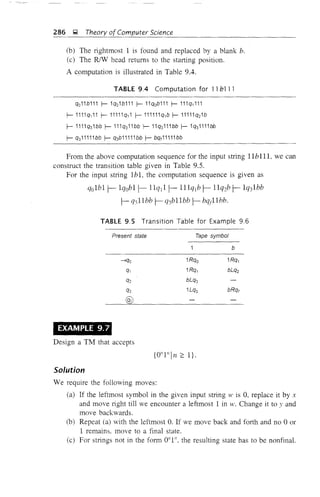

![288 g Theory ofComputer Science
Solution
Before designing the required Turing machine M, let us evolve a procedure for
processing the input stJing 112233. After processing, we require the ID to be
of the form bbbbbbq;. The processing is done by using five steps:
Step 1 qj is the initial state. The RJW head scans the leftmost 1, replaces 1
by b, and moves to the right. M enters q2'
Step 2 On scanning the leftmost 2, the RJW head replaces 2 by b and moves
to the right. M enters q3'
Step 3 On scanning the leftmost 3. the RJW head replaces 3 by b, and moves
to the right. M enters q4'
Step 4 After scanning the rightmost 3, the RJW heads moves to the left until
it finds the leftmost 1. As a result. the leftmost 1. 2 and 3 are replaced by b.
Step 5 Steps 1-4 are repeated until alll's, 2's and 3's are replaced by blanks.
The change of IDs due to processing of 112233 is given as
qj 112233 1-bq212233 1- blq22233 1- blbq3233 1- blb2q333
r-blb2bq..j31- blb2qsb3 1- b1bqs2b3 1- b1qsb2b3 1- bqs1b2b3
r-q6b1b2b31- bq]lb2b31- bbq2b2b3 1- bbbq22b3
r- bbbbq3b3 1- bbbbbq33 1- bbbbbbq..jb r- bbbbbq;bb
Thus.
q112233 ~ q7bbbbbb
As q7 is an accepting state, the input string 112233 is accepted.
Now we can construct the transition table for M. It is given in Table 9.6.
TABLE 9.6 Transition Table for Example 9.7
Present state Input tape symbol
2 3 b
-'>q., bRq2
q2 1Rq2 bRq3
q3 2Rq3 bRq4
q4 3Lqs
qs 1Lqa 2Lqs
qs 1Lqs
(~
bRq1
bRq2
bRq3
bLq7
bLQs
bRQ1
It can be seen from the table that strings other than those of the form 0"1"2"
are not accepted. It is advisable to compute the computation sequence for
strings like 1223, 1123. 1233 and then see that these strings are rejected by M.](https://image.slidesharecdn.com/automata-150510143406-lva1-app6891/85/Automata-301-320.jpg)
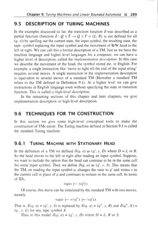
![290 );l Theory of Computer Science
9.6.2 STORAGE IN THE STATE
Weare using a state, whether it is of a FA or pda or TM, to 'remember' things.
We can use a state to store a symbol as well. So the state becomes a pair
(q, a) where q is the state (in the usual sense) and a is the tape symbol stored
in (q, a). So the new set of states becomes Q x r.
EXAMPLE 9.9
Construct a TM that accepts the language 0 1* + 1 0*.
Solution
We have to construct a TM that remembers the first symbol and checks that it
does not appear afterwards in the input string. So we require two states, qa, qj.
The tape symbols are 0, 1 and b. So the TM, having the 'storage facility in
state'. is
M = ({qa, qd x {O. L b}, {O, I}, {O, 1, b}, 0, [cIa, b], {[Cf], bJ})
We desClibe 0 by its implementation description.
L In the initial state, M is in qa and has b in its data portion. On seeing
the first symbol of the input sting w, M moves right, enters the state
Cft and the first symbol. say a, it has seen.
2. M is now in [q], a). (i) If its next symbol is b, M enters [cIt- b), an
accepting state. (ii) If the next symbol is a, M halts without reaching
the final state (i.e. 0 is not defined). (iii) If the next symbol is a
(a =°if a =1 and a =1 if a =0), M moves right without changing
state.
3. Step 2 is repeated until M reaches [qj, b) or halts (0 is not defined for
an input symbol in vv).
9.6.3 MULTIPLE TRACK TURING MACHINE
In the case of TM defined earlier, a single tape was used. In a multiple track
TM. a single tape is assumed to be divided into several tracks. Now the tape
alphabet is required to consist of k-tuples of tape symbols, k being the number
of tracks. Hence the only difference between the standard TM and the TM with
multiple tracks is the set of tape symbols. In the case of the standard Turing
machine, tape symbols are elements of r; in the case of TM with multiple track,
it is rk
. The moves are defined in a similar way.
9.6.4 SUBROUTINES
We know that subroutines are used in computer languages, when some task has
to be done repeatedly. We can implement this facility for TMs as well.](https://image.slidesharecdn.com/automata-150510143406-lva1-app6891/85/Automata-303-320.jpg)

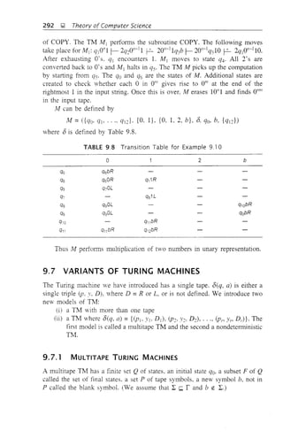
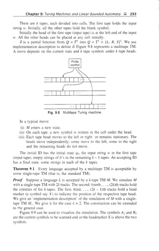

![Chapter 9: Turing Machines and Linear Bounded Automata J; 295
Proof Let AI be a k-tape TM. After 11 moves of M, the head markers of M]
will be separated by 211 cells or less. (At the worst. one tape movement can be
to the left by 11 cells and another can be to the right by II cells. In this case the
tape headmarkers are separated by 211 cells. In the other cases, the 'gap'
between them is less). To simulate a move of M, the TM M] must visit all the
k headmarkers. If M starts with the leftmost headmarker, M I will go through all
the headmarkers by moving right by at most 211 cells. To simulate the change
in each tape. M] has to move left by at most 271 cells; to simulate changes in
k tapes, it requires at most two moves in the reverse direction for each tape.
Thus the total number of moves by M 1 for simulating one move of M is
atmost 411 + 2k. (211 moves to light for locating all headmarkers, 211 + 2k moves
to the left for simulating the change in the content of k tapes.) So the number
of moves of M] for simulating n moves of M is 11(411 + 2k). As the constant k
is independent of 11, the time taken by M] is O(n:;).
9.7.2 NONDETERMINISTIC TURING MACHINES
In the case of standard Turing machines (hereafter we refer to this machine as
deterministic TM). 8(q). a) was defined (for some elements of Q x n as an
element of Q x r x {L R}. Now we extend the definition of 8. In a
nondetemlinistic TM. 8(ql, a) is defined as a subset of Q x r x {L R}.
Defmition 9.5 A nondeterministic Turing machine is a 7-tuple (Q, L r. 8, qo.
b. F) where
1. Q is a finite nonempty set of states
2. r is a finite nonempty set of tape symbols
3. b E r is called the blank symbol
4. L is a nonempty subset of 1. called the set of input symbols. We
assume that bEL.
5. qo is the initial state
6. F r;;;; Q is the set of final states
7. 8 is a partial function from Q x r into the power set of Q x r x
{L. R}.
1Vote: If q E Q and x E rand 8(q. x) = {(ql. :'), D 1). (q:;, .':;, D:;). ...,
(q", )'11' Dill) then the NTM can chose anyone of the actions defined by
(qi' )'i, DJ for i = 1. 2..... 11.
We can also express this in terms of f- relation. If 8(q. x) ={(qi, )ii, DJI
i =1. 2...., 11} then the ID zq.nv can change to anyone of the 11 IDs specified
by the l1-element set 8(q. x).
Suppose 8(q, x) ={(q], .'1, L). (q:;, ":;. R). (Q3, '3, L)}. Then
or
or](https://image.slidesharecdn.com/automata-150510143406-lva1-app6891/85/Automata-308-320.jpg)
![296 ~ Theory of Computer Science
So on reading the input symbol, the NTM M whose cun-ent ID is 2]2: ...
ZkqxZk+] ... 2/1 can change to anyone of the three IDs given earlier.
Remark When o(q, x) = {(qi' Yi, D i) Ii = 1. 2, .... n} then NTM chooses any
one of the n triples totally (that is, it cannot take a state from one triple, another
tape symbol from a second tliple and a third D(L or R) from a third triple, etc.
Definition 9.6 W E L* is accepted by a nondetenninistic TM M if qaw ~
xqfY for some final state qt.
The set of all strings accepted by M is denoted by T(M).
Note: As in the case of NDFA, an ID of the fonn xqy (for some q tt: F) may
be reached as the result of applying the input string w. But 'v is accepted by M
as long as there is some sequence of moves leading to an ID with an accepting
state. It does not matter that there are other sequences of moves leading to an
ID with a nonfinal state or TM halts without processing the entire input stling.
Theorem 9.3 If M is a nondeterministic TM, there is a deterministic TM Mj
such that T(M) = TUY!I)'
Proof We constmct M] as a multitape TM. Each symbol in the input string
leads to a change in ID. M] should be able to reach all IDs and stop when an
ID containing a final state is reached. So the first tape is used to store IDs of
M as a sequence and also the state of M. These IDs are separated by the symbol
* (induded as a tape symbol). The cun-ent ID is known by marking an x along
with the ID-separator * (The symbol * marked with x is a new tape symbol.)
All IDs to the left of the cun-ent one have been explored already and so can be
ignored subsequently. Note that the cun-ent ID is decided by the cun-ent input
symbol of w.
Figure 9.10 illustrates the deterministic TM M j •
Tape 1
Tape 2
x
101 * 102 * 103 * 104 * 105 * 106 * •.•
Fig. 9.10 The deterministic TM simulating M.
To process the current ID. M] perfOlIDs the follOving steps.
1. Mj examines the state and the scanned symbol of the cun-ent ID. Using
the knowledge of moves of M stored in the finite control of Mjo M]
checks whether the state in the cun-ent ID is an accepting state of M.
In this case M I accepts and stops simulating M.](https://image.slidesharecdn.com/automata-150510143406-lva1-app6891/85/Automata-309-320.jpg)
![Chapter 9: Turing Machines and Linear Bounded Automata J;! 297
2. If the state q say in the current ID xqa), is not an accepting state of M 1
and O(q, a) has k triples, M1 copies the ID xqay in the second tape and
makes k copies of this ID at the end of the sequence of IDs in tape 2.
3. M j modifies these k IDs in tape 2 according to the k choices given by
O(q, a).
4. M1 returns to the marked current ID. erases the mark x and marks the
next ID-separator * with x (to the * which is to the left of the next ID
to be processed). Then M j goes back to step 1.
M j stops when an accepting state of M is reached in step 1.
Now M 1 accepts an input string IV only when it is able to find that M has
entered an accepting state, after a finite number of moves. This is clear from
the simulated sequence of moves of M j (ending in step 1)
We have to prove that M j will eventually reach an accepting ID (that is,
an ID having an accepting state of M) if M enters an accepting ID after n
moves. Note each move of M is simulated by several moves of M j •
Let m be the maximum number of choices that M has for various (q, a)'s.
(It is possible to find m since we have only finite number of pairs in Q x r.)
So for each initial ID of M. there are at most m IDs that M can reach after one
move. at most m2
IDs that I'v! can reach after two moves. and so on. So
corresponding to n moves of M, there are at most 1 + m + m
2
+ ... + mil moves
of M 1• Hence the number of IDs to be explored by M 1 is at most nm".
We assume that M] explores these IDs. These IDs have a tree structure
having the initial ID as its root. We can apply breadth-first search of the nodes
of the tree (that is. the nodes at level 1 are searched. then the nodes at level 2,
and so on.) If At reaches an accepting ID after n moves. then M1 has to search
atmost nm/! IDs before reaching an accepting ID. So. if M accepts lV, then M 1
also accepts lV (eventually). Hence T(M) = T(Mj ).
9.8 THE MODEL OF LINEAR BOUNDED AUTOMATON
This model is important because (a) the set of context-sensitive languages is
accepted by the model. and (b) the infinite storage is restricted in size but not
in accessibility to the storage in comparison with the Turing machine model. It
is called the linear bounded automaton (LBA) because a linear function is used
to restrict (to bound) the length of the tape.
In this section we define the model of linear bounded automaton and
develop the relation between the linear bounded automata and context-sensitive
languages. It should be noted that the study of context-sensitive languages is
important from practical point of view because many compiler languages lie
between context-sensitive and context-free languages.
A linear bounded automaton is a nondetelministic Turing machine which
has a single tape whose length is not infinite but bounded by a linear function](https://image.slidesharecdn.com/automata-150510143406-lva1-app6891/85/Automata-310-320.jpg)

![Chapter 9: Turing Machines and Linear Bounded Automata ~ 299
that k changes to k - 1 if the RIW head moves to the left and to k + 1 if the
head moves to the right.
The language accepted by LBA is defined as the set
{w E (l: - {¢, $})*I(qo, ¢,v$, 1) rc- (q, ex, i)
for some q E F and for some integer i between 1 and n},
Note: As a null string can be represented either by the absence of input string
or by a completely blank tape, an LBA may accept the null string,
9.8.1 RELATION BETWEEN LBA AND CONTEXT-SENSITIVE
LANGUAGES
The set of strings accepted by nondeterministic LBA is the set of strings
generated by the context-sensitive grammars, excluding the null strings, Now
we give an important result:
If L is a context-sensitive language, then L is accepted by a linear bounded
automaton. The converse is also true.
The construction and the proof are similar to those for Turing machines
with some modifications.
9.9 TURING MACHINES AND TYPE 0 GRAMMARS
In this section we construct a type 0 grammar generating the set accepted by
a given Turing machine M. The productions are constructed in two steps. In
step 1 we construct productions which transform the string [ql¢ w$] into the
string [q2bJ, where qj is the initial state, q2 is an accepting state, ¢ is the left-
endmarker. and $ is the right-endmarker. The grammar obtained by applying
step 1 is called the transfonnational grammar. In step 2 we obtain inverse
production rules by reversing the productions of the transformational grammar
to get the required type 0 grammar G. The construction is in such a way that
11' is accepted by M if and only if w is in L(G).
9.9.1 CONSTRUCTION OF A GRAMMAR CORRESPONDING
TO TM
For understanding the construction. we have to note that a transition of ID
corresponds to a production. We enclose IDs within brackets. So acceptance of
, by M corresponds to the transformation of initial ID [ql ¢ W $] into [q2b].
Also, the 'length' of ID may change if the RIW head reaches the left-end or the
right-end, i.e. when the left-hand side or the right-hand side bracket is reached.
So we get productions corresponding to transition of IDs with (i) no change in
length, and (ii) change in length, We assume that the transition table is given,](https://image.slidesharecdn.com/automata-150510143406-lva1-app6891/85/Automata-312-320.jpg)
![300 ~ Theory of Computer Science
We now describe the construction which involves two steps:
Step 1 (i) No change in length of IDs: (a) Right move. akRqt corresponding
to qt-row and arcolumn leads to the production
qta) -+ ak-Cft
(b) Left move. akLqt cOlTesponding to qt-row and arcolumn yields several
productions
for all am E r
(ii) Change in length of IDs: (a) Left-end. akLqt cOlTesponding to q/-row
and arcolumn gives
[q;a; -+ [cltbak
When b occurs next to the left-bracket, it can be deleted. This is achieved
by including the production [b -+ [.
(b) Right-end. When b occurs to the left of ], it can be deleted. This is
achieved by the production
a;b] -+ a;J for all aj E r
When the RJW head moves to the right of ], the length mcreases.
Corresponding to this ve have a production
q;] -+ qtb] for all qt E Q
(iii) lmrodllction ofendmarkers. For introducing endmarkers for the input
string, the following productions are included:
at -+ [qj ¢ a; for at E r. at 1= b
for all at E r, at 1= b
For removing the brackets from [q2b], we include the production
[q2b] -+ S
Recall that qj and q2 are the initial and final states, respectively.
Step 2 To get the required grammar, reverse the arrows of the productions
obtained in step 1. The productions we get can be called inverse productions.
The new grammar is called the generative grammar. We illustrate the
construction 'lith an example.
EXAMPLE 9.11
Consider the TM described by the transition table given in Table 9.9. Obtain
the inverse production rules.
Solution
In this example. qj is both initial and final.
Step 1 (i) Prodllctions corresponding to right moves
(9.1)](https://image.slidesharecdn.com/automata-150510143406-lva1-app6891/85/Automata-313-320.jpg)
![Chapter 9: Turing Machines and Linear Bounded Automata ~ 301
(ii) (a) Productions corresponding to left-end
[b ~ [
(b) Productions corresponding to rig',ot-end
(9.2)
bb] ~ b],
(iii) 1 ~ [qj¢1,
lb] ~ 1],
1 ~ IS],
ql] ~ qlb],
[qlb] ~ S
(9.3)
(9.4)
TABLE 9.9 Transition Table for Example 9.11
Present state b
Step 2 The inverse productions are obtained by reversing the arrows of the
productions (9.1)-(9.4).
¢ql ~ ql¢ bq~ ~ ql l, bql ~ q~l
[ ~ [b, b] ~ bb], 1] ~ lb]
qlb ~ ql], q~b ~ q~]. [cII¢l ~ 1
1$] ~ 1, S ~ [q1b]
Thus we have shown that there exists a type 0 grammar corresponding to
a Turing machine. The converse is also true (we are not proving this), i.e. given
a type 0 grammar G. there exists a Tming machine accepting L(G). Actually,
the class of recursively enumerable sets, the type 0 languages, and the class of
sets accepted by TM are one and the same. We have shown that there exists
a recursively enumerable set which is not a context-sensitive language (see
Theorem 4.4). As a recursive set is recursively enumerable, Theorem 4.4 gives
a type 0 language which is not type 1. Hence, 4s1 c.~ (d Property 4,
Section 4.3) is established.
9.10 LINEAR BOUNDED AUTOMATA AND LANGUAGES
A linear bounded automaton M accepts a string w if. after starting at the initial
state with RIW head reading the left-endmarker, M halts over the right-end-
marker in a final state. Otherwise, w is rejected.
The production rules for the generative grammar are constructed as in the
case of Turing machines. The following additional productions are needed in
the case of LBA.
Qiqr$ ~ qf$
¢lrS ~ ¢qr,
for all Qi E r
¢qf ~ qt](https://image.slidesharecdn.com/automata-150510143406-lva1-app6891/85/Automata-314-320.jpg)
![302 g Theory of Computer Science
EXAMPLE 9.12
Find the grammar generating the set accepted by a linear bounded automaton
M whose transition table is given in Table 9.10.
TABLE 9.10 Transition Table for Example 9.12
Present state Tape input symbol
~ $ 0
---7q1 ~Rq1 1Lq2 ORq2
q2 ~Rq4 1Rq3 1Lq1
q3 $Lq1 1Rq3 1Rq3.
® Halt OLq4 ORq4
Solution
Step 1 (A) (i) Productiolls corresponding to right moves. The seven right
moves in Table 9.10 give the following productions:
(9.5)
q30 ~ lq3
q3 1 ~ lq3
q.+l ~ Oq.+
qlc): ~ c):qj.
qjl ~ OC):.
q:c): ~ C):C).+,
q:O ~ lq3
(ii) Productions corresponding to left moves. There are four left moves in
Table 9.10. Each left move yields four productions (corresponding to the four
tape symbols). These are:
(a) lLq: corresponding to ql-row and O-column gives
c):qjO ~ q:¢l, SqjO ~ C)2$}, OqlO ~ q201, lq j O ~ q211 (9.6)
(b) lLql corresponding to qj-rmv and I-column yields
¢q:l ~ ql¢l, Sq:l ~ qjSL Oq:l ~ ql0!, lq:l ~ qlll (9.7)
(c) SLqj corresponding to qrroV and $-column gives
c):q3$ ~ qj¢$, Sq3$ ~ CJlS$, 0CJ3$ ~ CJjO$, lCJ3$ ~ CJll$ (9.8)
(d) OLq.+ corresponding to CJ.+-row and O-column yields
¢CJ.+O ~ CJ.+¢O, $q.+O ~ q.+$O, Oq.+O ~ q.+OO, lq.+O ~ q410 (9.9)
(B) There are no productions corresponding to change in length.
(C) The productions for introducing the endmarkers are
¢~ [C)l¢¢
$ ~ [CJ1¢$,
°~ [(1J¢0,
1 ~ [ql¢L
[q.+] ~ S
¢ -+ ¢$]
$ ~ $$]
°~ OS]
1 ~ 1$]
(9.10)
(9.11)](https://image.slidesharecdn.com/automata-150510143406-lva1-app6891/85/Automata-315-320.jpg)


![Chapter 9: Turing Machines and Linear Bounded Automata ~ 305
where 8 is defined by
8(qo, 0) =(e/j, 0, R)
8(q], 0) = (qj, 0, R)
8(q], b) =(q2' b, L)
8(q2, 0) =(q3' b, L)
8(q3' 0) =(q3' 0, L)
8(q3' b) = (q4' b, R)
8(qo, 1) =(qj, 1, R)
8(qj' 1) = (ql' 1, R)
8(q2' 1) =(q3' b, L)
8(q3' 1) = (q3' 1, L)
(R])
(R2)
(R3)
(R4)
(Rs)
(~)
Let w be the input string, By (R]) and (R2), M reads the entire input string
w. At the end, M is in state qj' On seeing the blank to the right of w, M reaches
the state q2 and moves left. The rightmost string in w is erased (by (R4)) and
the state becomes q3' Afterwards M moves to the left until it reaches the left-
end of w, On seeing the blank b to the right of w, M changes its state to q4'
which is the final state of M. From the construction it is clear that the rightmost
symbol of w is erased.
EXAMPLE 9.16
Construct a TM that accepts L = {02
1i
I11 2: O}.
Solution
Let ,v be an input string in {O} *. The TM accepting L functions as follows:
1. It wlites b (blank symbol) on the leftmost 0 of the input string w. This
is done to mark the left-end of w.
2. M reads the symbols of w from left to right and replaces the alternate
O's with x's.
3. If the tape contains a single 0 in step 2, M accepts w.
4. If the tape contains more than one 0 and the number of O's is odd in
step 2, M rejects w.
5. M returns the head to the left-end of the tape (marked by blank b in
step 1).
6. M goes to step 2.
Each iteration of step 2 reduces w to half its size. Also whether the number
of O's seen is even or odd is known after step 2. If that number is odd and
greater than 1, IV cannot be 02
1i
(step 4). In this case M rejects w. If the number
of 0's seen is 1 (step 3), M accepts w (In this case 0
211
is reduced to 0 in
successive stages of step 2).
We define M by
M = ({qo, qj, (f2, q3' q4' ql' ql}, {O}, {O, x, b}, 8, qo, b, {qiD
where 8 is defined by Table 9.12.](https://image.slidesharecdn.com/automata-150510143406-lva1-app6891/85/Automata-318-320.jpg)
![306 J;I, Theory ofComputer Science
TABLE 9.12 Transition Table for Example 9.16
Present state Tape symbol
0 b .r
qo bRq1 bRqt xRqt
q1 .rRq2 bRqf xRq1
q2 ORq3 bRq4 xRq2
q3 xRq2 bRq6 xRq3
q4 OLQ4 bRQ1 xLQ4
Qr
Qt
From the construction, it is apparent that the states are used to know
whether the number of O's read is odd or even.
We can see how M processes 0000.
qoOOOO ~ bCf1000 ~ bJ.(1200 ~ b.xxl30 ~ bX{)XCf2b
~ bxOq.+xb ~ bxq.+Oxb ~ bq4--r:Oxb ~ q4bxOxb
~ bq1xO.-r:b ~ bxq10xb ~ bx.-r:Cf2Xb ~ bxxxq2b
~ bxxq4xb ~ bxq.+xxb ~ bqJ,xxxb ~ qJ,bxxxb
~ bqlxxxb ~ bXqlxxb ~ bxxqjxb ~ bxxxqjb
~ bxxxbCfI'
Hence M accepts i'.
Also note that M always halts. If M reaches qt, the input stling 11' is
accepted by M. If M reaches qr- }t' is not accepted by M; in this case M halts
in the trap state.
EXAMPLE 9.17
Let M = ({qo, qj, q2}. {O. I}. {O, 1, b}. 8, qo, {q2})
where 8 is given by
8(qo, 0) = (qj, 1, R)
8(qj, 1) = (qo- 0, R)
8(qj. b) =(q2' b, R)
(Rj )
(R2)
(R3)
Find T(M),
Solution
Let 11' E T(M), As 8(qo, 1) is not defined, w cannot start with 1. From (Rd
and (R2), we can conclude that M starts from qo and comes back to Cfo after
reaching 01.
So. qo(OI)" f-2- (lO)"qo· Also, qoOb ~ lq]b ~ Ibq2'](https://image.slidesharecdn.com/automata-150510143406-lva1-app6891/85/Automata-319-320.jpg)
![Chapter 9: Turing Machines and Linear Bounded Automata J;! 307
So, (On"O E T(M). Also, (OltO is the only string that makes M move from
qo to Cf~· Hence, T(M) = {(Olto In;:: O}.
SELF-TEST
Choose the correct answer to Questions 1-10:
1. For the standard TM:
(a) L =r
(b) r <;:;;; L
(c) L <;:;;; r
(d) L is a proper subset of r.
2. In a standard TM. D(q. a), q E Q, a E r is
(a) defined for all (q. a) E Q x r
(b) defined for some. not necessarily for all (q, a) E Q x r
(c) defined for no element (q. a) of Q >< r
(d) a set of triples with more than one element.
3. If D(q. .J = (p. Y. I), then
(a) XlX~ Xi-lqxi x" ~ XIX2 xi_~pxi_l.vxi+l ... .en
(b) XIX~ xi_lqxi x" ~ Xl.Y2 'Yi-lYi'JXi+I ... x"
(c) XIX~ xi_IqXi XI) ~ XI ·'(i-3P.Yi-~Xi-1YXi+l ... XII
(d) XIX~ xi-lqxi XII ~ XI Xi+J1T'Xi+~ ... Xn
4. If D(q. X;) =(p. y. R). then
(a) XIX~ 'Yi-lqxi Xii ~ XIX~ Xi-lypXi+l x"
(b) X1X~ xi-lqxi Xli ~ X)X2 XiPXi+l .1'1/
(e) X,X2 xi-lq'Yi X" ~ X)'Y2 Xi-1PXiXi+l x"
(d) X!X~ Xi-1CfXi X1/ ~ .1'1"2 Xi-lypXi+J X1/
5. If D(q. Xl) =(p, y. I). then
(a) qXlx~ Xii ~ p.vX~ Xli
(b) q.YIX~ X" ~ yp.Y~ Xli
(e) qXJX~ X" ~ pbx] XI1
(d) qx(r~ X" ~ pbx~ x"
6. If D(q. xl1
) = (v. Y. R). then
(a) Xl ... x n_lqx" ~ PYX2J:3 Xn
(b) x • ... X1/-1q·, p:- PYX~X3 XII
(c) Xl x n_lqxl1 ~ XIX~ X"_l)pb
(d) Xl X"_lqx,, p:- XIX~ xn_lypb
7. For the TM given in Example 9.6:
(a) qolbll p:- bqj llbbl
(b) qn lbll i- bqrllbhl
(c) Cj(Jlbll ~ lqoblll
(d) Cjolbll ~ (j3bllbbl](https://image.slidesharecdn.com/automata-150510143406-lva1-app6891/85/Automata-320-320.jpg)


![Chapter 10: Decidability and Recursively Enumerable Languages I;! 311
Definition 10.4 A problemflanguage is undecidable if it is not decidable.
Note: A decidable problem is called a solvable problem and an undecidable
problem an unsolvable problem by some authors.
10.3 DECIDABLE LANGUAGES
In this section we consider the decidability of regular and context-free
languages.
First of all. we consider the problem of testing whether a detenninistic
finite automaton accepts a given input string lV,
Definition 10.5
Am; = {(B, lV) IB accepts the input string w}
Theorem 10.1 ADFA is decidable.
Proof To prove the theorem. we have to construct a TM that always halts
and also accepts ADf.-' We describe the TM M using high level description
(refer to Section 9.5). Note that a DFM B always ends in some state of B after
n transitions for an input string of length n.
We defme a TM M as follows:
1. Let B be a DFA and w an input string. (B, w) is an input for the Turing
machine M.
2. Simulate B and input H' in the TM M.
3. If the simulation ends in an accepting state of B. then M accepts w.
If it ends in a nonaccepting state of B, then M rejects w.
We can discuss a few implementation details regarding steps 1. 2 and 3
above. The input (B, H') for 11 is represented by representing the five
components Q, L, 8, qo, f by strings of L* and input string W E L*. M checks
whether (B. w) is a valid input. If not. it rejectes (B, w) and halts. If (B, w)
is a valid input. ['vi writes the initial state qo and the leftmost input symbol of
w. It updates the state using 0 and then reads the next symbol in w. This
explains step 2.
If the simulation ends in an accepting state w' then M accepts (B, w)..
Otherwise, Iv! rejects (B, IV). This is the description of step 3.
It is evident that M accepts (B, if and only if H' is accepted by the
DFA B. I
Definition 10.6
ACFG = {(G, w) i the context-free grammar G accepts the input string w}
Theorem 10.2 ACFG IS decidable.
Proof We convert a CFG into Chomsky 110lmal form. Then any derivation
of H' of length k requires 2k - 1 steps if the grammar is in C]IF (refer
to Example 6.18). So for checking whether the input string ft of length k is](https://image.slidesharecdn.com/automata-150510143406-lva1-app6891/85/Automata-324-320.jpg)

![Chapter 10: Decidahility and Recursively Enumerahle Languages l;l 313
10.4 UNDECIDABLE LANGUAGES
In this section we prove the existence of languages that are not recursively
enumerable and address the undecidability of recursively enumerable
languages.
Theorem 10.4 There exists a language over 2: that is not recursively
enumerable.
Proof A language L is recursively enumerable if there exists a TM M such
that L =T(M). As L is finite, 2:* is countable (that is, there exists a one-to-
one correspondence between 2:* and N).
As a Turing machine M is a 7-tuple (Q. 2:, f', 8, qo. b, F) and each
member of the 7-tuple is a finite set M can be encoded as a string. So the
set I of all TMs is countable.
Let J: be the set of all languages over 2:. Then a member of J: is a subset
of P (Note that P is infinite even though I is finite), We show that ;i is
uncountable (that is, an infinite set not in one-to correspondence with N).
We prove this by contradiction. If ;L were countable then J: can be
written as a sequence {L[, L2• L3, ... }. We Tite 2:* as a sequence {11']. W2'
We, . ... }. So Li can be represented as an infinite binary sequence XnXi2Xi3' ..
where
r1 ihv} E L;
lO otherwise
Using this representation we write L; as an infinite binary sequence.
L] XI]X12X 13 x]i
L, x2I x ::x :3 x:}
Li Xil Xi2Xi3 xi)
Fig. 10.1 Representation of T
We define a subset L of 2:* by the binary sequence ."].":."3 ... where Y; =
1 - Xii' If Xii =0, Yi =1 and if Xii =I, ."; =O. Thus according to our assumption
the subset L of I* represented by the infinite binary sequence YIY:Y3 ...
should be Lk for some natural number k. But L =f. Lt. since Wk E L if and only
if Hk It: Lk~ This contradicts our assumption that ci is countable. Therefore 1.
is uncountable. As J is countable. ;L should have some members not
corresponding to any TM in 1. This proves the existence of a language over
2: tnat is not recursively enumerable. I
Defmition 10.8 ATM = {(M, w) IThe TM M accepts w}.](https://image.slidesharecdn.com/automata-150510143406-lva1-app6891/85/Automata-326-320.jpg)


![Chapter 10: Decidability and Recursively Enumerable Languages Q 317
We state the following theorem by Emil Post without proof.
Theorem 10.7 The PCP over 2: for 12:1 ;::: 2 is unsolvable.
It is possible to reduce the PCP to many classes of two outputs
(yes/no) problems in formal language theory. The following results can be
proved by the reduction technique applied to PCP.
1. If L1 and L2 are any two context-free languages (type 2) over an
alphabet 2: and 12:1 ;::: 2, there is no algorithm to determine whether or
not
(a) L] (l L2 = 0,
(b) L1 (l L2 is a context-free language,
(c) L] k L2, and
(d) L1 =L2•
2. If G is a context-sensitive grammar (type 1), there is no algorithm to
determine whether or not
(a) L(G) = 0,
(b) L(G) is infinite, and
(c) Xo E L(G) for a fixed string Xcr
3. If G is a type 0 grammar, there is no algorithm to determine whether
or not any string x E 2:* is in L(G).
10.7 SUPPLEMENTARY EXAMPLES
EXAMPLE 10.4
If L is a recursive language over 2:, show that I (I is defined as 2:* - L) is
also recursive.
Solution
As L is recursive, there is a Turing machine M that halts and T(M) =L. We
have to construct a TM M 1, such that T(M1) = [ and M 1 eventually halts.
M] is obtained by modifying M as follows:
1. Accepting states of M are made nonaccepting states of MI'
2. Let M 1 have a new state qf After reaching qfi M] does not move in
further transitions.
3. If q is a nonaccepting state of M and 6(q, x) is not defined, add a
transition from q to qf for lvh
As M halts, M 1 also halts. (If M reaches an accepting state on w, then M]
d.~es not accept wand halts and conversely.)
Also M] accepts w if and only if M does not accept w. So I is recursive.](https://image.slidesharecdn.com/automata-150510143406-lva1-app6891/85/Automata-330-320.jpg)
![318 );;,] Theory ofComputer Science
EXAMPLE 10.5
If Land L are both recursively enumerable. show that Land L are recursive.
Solution
Let M 1 and M 2 be two TMs such that L =T(M1) and L =T(M2). We construct
a new two-tape TM M that simulates M] on one tape and M2 on the otheL
If the input string w of M is in L, then M1 accepts wand we declare that
M accepts w. If w E [, then M2 accepts wand we declare that M halts without
accepting. Thus in both cases, M eventually halts. By the construction of M
it is clear that T(lvl) =T(M]) =L Hence L is recursive. We can show that
[ is recursive, either by applying Example lOA or by interchanging the roles
of M) and M 2 in defining acceptance by M.
EXAMPLE 10.6
Show that ATM
is not recursively enumerable.
Solution
We have already seen that Anv! is recursively enumerable (by Theorem 10.5).
If itTIY! were also recursively enumerable, then ATM is recursive (by
Example 10.5). This ~ a contradiction since ATM is not recursive by
Theorem 10.5. Hence A TM is not recursively enumerable,
EXAMPLE 10.7
Show that the union of two recursively enumerable languages is recursively
enumerable and the union of two recursive languages is recursive.
Solution
Let L 1 and L2 be two recursive languages and M 1, M2 be the corresponding
TMs that halt. We design a Th1 M as a two-tape TM as follows:
1. w is an input string to M.
2. M copies ,von its second tape.
3. M simulates M) on the first tape. If w is accepted by M10 then M
accepts ,v.
4. M simulates /'112 on the second tape. If w is accepted by M2, then M
accepts w.
M always halts for any input w.
Tnus LJ U L2 = T(M) and hence LJ
U L2 is recursive.
If L) and L2 are recursively enumerable. then the same conclusion gives
a proof for L) U L2 to be recursively enumerable. As M 1 and M2 need not
halt, M need not halt.](https://image.slidesharecdn.com/automata-150510143406-lva1-app6891/85/Automata-331-320.jpg)

![Chapter 10: Decidability and Recursively Enumerable Languages g 321
10.18 Prove that PCP is solvable if Il: I = l.
10.19 Let x =(Xl' .. X,,) and Y =(YI ... y,,) be two lists of nonempty strings
over l: and Il: I2: 2. (i) Is PCP solvable for n =I? (ii) Is PCP solvable
for n = 2?
10.20 Prove that the PCP with {(01, 011), (1, 10), (I,ll)} has no solution.
(Here, Xl =01, X2 = 1, X3 = 1, YI =011, 1'2 = 10, Y3 = 11.)
10.21 Show that the PCP with S = {(O, 10), (12
0, 03
), (02
1, IOn has no
solution. [Hint: No pair has common nonempty initial substring.]
10.22 Does the PCP with X =(b3
, ab2
) and Y =(b3
, bab3
) have a solution?
10.23 Find at least three solutions to PCP defined by the dominoes:
1
10m
I
10
10.24 (a) Can you simulate a Turing machine on a general-purpose
computer? Explain.
(b) Can you simulate a general-purpose computer on a Turing
machine'? Explain.](https://image.slidesharecdn.com/automata-150510143406-lva1-app6891/85/Automata-334-320.jpg)
 = 4, U?(2, 4, 7) =2, utO, 4, 7)
_ '7
- I
TABLE 11,1 Initial Functions Over tv
Zero function Z defined by Z(x) = 0,
Successor function S defined by S(x) = x + 1
Projection function U/" defined by Ur"(.'1 "" xn) = x"
Note: As Ul(x) = x for every x in N. ui is simply the identity function. So
Uf' is also termed a generalized identity function.
The initial functions over L are given in Table 11.2. In pmticular,
nil (abab) = A
cons a(abab) =aabab
cons b(abab) = babab
Note: We note that cons a(x) and cons b(x) simply denote the concatenation
of the 'constant' string a and X and the concatenation of the constant string
band x.
TABLE 11.2 Initial Functions Over {a, b}
nil (x) = A
cons a(x) = ax
cons b(x) = bx](https://image.slidesharecdn.com/automata-150510143406-lva1-app6891/85/Automata-336-320.jpg)

![Chapter 11: Computahility J;;;! 325
The next definition gives a mechanical process of computing a function.
Definition 11.2 A function f(x) over N is defined by recursion if there exists
a constant k (a natural number) and a function hex, y) such that
flO) =k, fen + 1) = hen, fin)) (11.1)
By induction on n, we can define fen) for all n. As f (0) =k, there is basis
for induction. Oncef(n) is known,f(n + 1) can be evaluated by using (11.1).
E;XAMPLE 11.4
Define n! by recursion.
Solution
flO) = 1 and fen + 1) = hen, fen)), where hex, y) = Sex) * y.
The above definition can be generalized for f(x]o X2, ..., Xll' X,,+I)' We
fix n variables in f(XI, X2, ..., XII+I), say. XI, X2, ..., XII" We apply Definition
11.2 to f(x], X2, ..., XII' y). In place of k we get a function g(Xlo X2, ..., XII)
and in place of hex, y), we obtain hex], X2, ..., X", y, f(x], ..., Xll' y)).
Definition 11.3 A function f of n + 1 variables is defined by recursion if
there exists a function g of n variables, and a function lz of n + 2 variables,
and f is defined as follows:
fCx:], X2• ..., XII' 0) = g(x]. X2, .... x,,) (11.2)
f(x] ... XII' Y + 1) = h(x]o X2, ..., X'I' y, f(XI, X2, ..., Xll' y)) (11.3)
We may note that f can be evaluated for all arguments (x]o X2, ..., x"' y)
by induction on y for fixed Xj. X2, ..., X/1" The process is repeated for every
Xl' X2, .... XII"
Now ve can define the primitive recursive functions over N.
11.2.2 PRIMITIVE RECURSIVE FUNCTIONS OVER N
Definition 11.4 A total function f over N is called primitive recursive
(i) if it is anyone of the three initial functions, or (ii) if it can be obtained
by applying composition and recursion a finite number of times to the set of
initial functions.
EXAMPLE 11.5
Show that the function fl(X, y) =X + Y is ptimitive recursive.
Solution
fl is a function of two variables. If we want f] to be defined by recursion, we
need a function g of a single variable and a function h of three variables.
fleX, 0) =X + 0 = x](https://image.slidesharecdn.com/automata-150510143406-lva1-app6891/85/Automata-338-320.jpg)
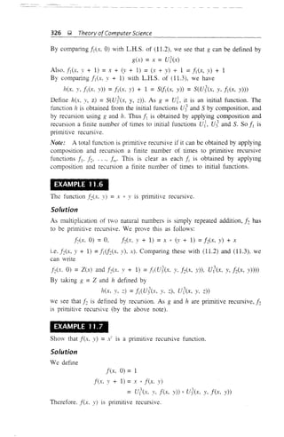

![Chapter 11: Computability ~ 329
concat(ax], X2) =cons a (concat(xb X2))
concat(bx], X2) =cons b (concat(x], X2))
SO concat is defined by recursion using id, cons a and cons b.
Therefore, concat is primitive recursive.
(d) The transpose function can be defined by trans(x) = xT
. Then
trans(A) = A
trans(ax) = concat(trans(x), a(x))
trans(bx) = concat(trans(x), b(x))
Therefore, trans(x) is primitive recursive.
(e) The head function head(x) satisfies
head(A) =A
head(ax) = a(x)
head(bx) = b(x)
Therefore, head(x) is primitive recursive.
(f) The tail function tail(x) satisfies
tail(A) =A
tail(ax) = id(x)
tail(bx) =id(x)
Therefore, tailex-) is pnm]t]ve recursive.
(g) The conditional function can be defined by
cond(x], X2, X3) = "if x] "* A then X:; else X3"
Then,
cond(A, Xb x3) = id(x3)
cond(ax], X:;, X3) = id(x:;)
cond(bx], X2, X3) = id(x:;)
Therefore, id(x], x2. :"3) is primitive recursive.
11.3 RECURSIVE FUNCTIONS
By introducing one more operation on functions, we define the class of
recursive functions, which includes the class of primitive recursive functions.
Def"mition 11.8 Let g(x], X2' ..., X/1' y) be a total function over N. g is a
regular function if there exists some natural number Yo such that g(x], X2, .. ",
XII' Yo) = 0 for all values X], X2, ..., X/1 in N.](https://image.slidesharecdn.com/automata-150510143406-lva1-app6891/85/Automata-342-320.jpg)
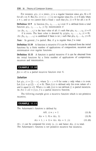


![Chapter 11: Computability l;;! 333
11.4.2 A TURING MODEL FOR COMPUTATION
As in the model introduced in Chapter 9, Q, qo and r denote the set of states.
the initial state, and the set of tape symbols, respectively. The blank symbol b
is in r. The only difference is in the transition function. In the present model
the transition function represents only one of the following three basic
operations:
(i) Writing a new symbol in the cell scanned
(ii) Moving to the left cell
(iii) Moving to the right cell
Each operation is followed by a change of state. Suppose the Turing machine
M is in state q and scans ai' If ai is written and M enters q', then this basic
operation is represemed by the quadruple qaiad. Similarly. the other two
operations are represented by the quadruples qaiLq' and qaiRq'. Thus the
transition function can be specified by a set P of quadruples. As in Chapter 9.
we can define instantaneous descriptions, i.e. IDs.
Each quadruple induces a change of IDs. For example, qa;ajq' induces
P. ' , [3CI.qail-' I aq ai
The quadruple qaiLq' induces
and qaiRq' induces
When we require M to perform some computation, we 'feed' the input by
initial tape expression denoted by X. So qaX is the initial ID for the given
input. For computing with the given input X. the Turing machine processes
X using appropriate quadruples in P. As a result. we have qoX =IDi r- ID2
r- .... When an ID. say IDil' is reached. which cannot be changed using any
quadruple in P, M halts. In this case, ID" is called a terminal ill. Actually,
aqj a[3 is a terminal ID if there is no quadruple starting with qi{l. The terminal
ID is called the result of X and denoted by Res(X). The computed value
cOlTesponding to input X can be obtained by deleting the state appeming in it
as also some more symbols from Res(X).
11.4.3 TURING-COMPUTABLE FUNCTIONS
Before developing the concept of Turing-computable functions. let us recall
Example 9.6. The TM developed in Example 9.6 concatenates two strings a
aej [3. Initially, a and [3 appear on the input tape separated by a blank b.
Finally, the concatenated string a[3 appears on the input tape. The same
method can be adopted with slight modifications for computing I(x] , ..., x,,')'
Suppose we want to construct a TM which can compute I(xl' ..., XII,) over](https://image.slidesharecdn.com/automata-150510143406-lva1-app6891/85/Automata-346-320.jpg)
![334 ~ Theory ofComputer Science
N for given arguments a], .... am' Initially, the input OJ, a2' ..., am appears
on the input tape separated by markers Xj, ... , Xlii' The computed value
f(a] , ..., am)' say, c appears on the input tape, once the computation is over.
To locate c ,ve need another marker. say y. The value c appears to the right
of X m and to the left of v. To make the construction simpler, we use the tally
notation to represent the elements of N. In the tally notation, 0 is represented
by a string of b's. A positive integer n is represented by a string consisting
of II 1's. So the initial tape expression takes the form 1"lx,1{/2x: ... 1{/mxmby.
As a resulr of computation, the initial ID qOFtxll"2X2 ... l{/lI/xlII by is changed
to a terminal ID of the form 1{/lXl1{/2X: ... 11lmx",1'q'y for some q' E Q. In
fact, the position of q' in a tenninal ID is immaterial and it can appear
anywhere in Res(X). The computed value is found between XIII and y.
Sometimes we may have to omit the leading b's.
We say that a function f(x] . ..., x",) is Turing-computable for arguments
aj, .... (1m if there exists a Turing machine for which
where IDII
is a terminal ID containing f(al' ..., alii) to the left of y.
Our ultimate aim is to prove that partial recursive functions are Turing-
computable. For this purpose. first of all we prove that the three initial primitive
recursive functions are Turing-computable.
11.4.4 CONSTRUCTION OF THE TURING MACHINE THAT
CAN COMPUTE THE ZERO FUNCTION Z
The zero function Z is defined as Zeal) = 0 for all al :::: O. So the initial tape
expression can be taken as X = 11l'xlby. As we require the computed value
Zeal)' namely O. to appear to the left of y, we require the machine to halt
without changing the input. (Note that 0 IS represented by b in the tally
notation.)
Thus we define a TM by taking Q = {qo, qd, r = {b. LXI_ Y},
X = l"jx,by. P consists of qobRqo, qolRqo. q(~llx1ql' qobRqo and qolRqo are
used to move to the right until Xl is encountered. q~llx1ql enables the TM to
enter the state ql' M enters qj without altering the tape symbol. In terms of
change of IDs. we have
a l"lx by f.2- l"la-li bv L- l"I('IX by10 I . ; 1(} . . I 1. , .
As there is no quadruple starting with ql' M halts and Res(X) =11Ij(11X1by.
By deleting ql in Res(X), we get l"lxlby (which is the same as X) yielding 0
(given by b).
Note: We can also represent the quadruples in a tabular form which is
similar to the transition table obtained in Chapter 9. In this case we have to
specify (i) the new symbol written. or (ii) the movement to the left (denoted
by L/. or (iii) the movement to the right (denoted by R). So we get
Table 11.3.](https://image.slidesharecdn.com/automata-150510143406-lva1-app6891/85/Automata-347-320.jpg)
![Chapter 11: Computability g 335
TABLE 11.3 Representation of Quadruples
State b y
r = {h. 1. Xj. y},
11.4.5 CONSTRUCTION OF THE TURING MACHiNE FOR
COMPUTING-THE SUCCESSOR FUNCTION
The successor function S is defined by Sea)) = aj + 1 for all aj 2': O. So the
initial tape expression can be taken as X =1({lX1by (as in the case of the zero
function). At the end of the computation. we require 1([1+
1
to appear to the left
of Y. Hence we define a TM by taking
Q = {qo. .. " q9},
where P consists of
(i) qobRqo. qolbql' q(}"t!Rqc;
(ii) q1bRqj. qjlRqj. qlxjRqj. qj'lq~
(iii) q~ lRq~. C]~byq3'
(iy) q3bLq3' q31Lq3' q3yLq3. q,X1Lq.+
(v) qJ,lLqJ,. C]J,blq).
(vi) q)lRqo.
(vii) qc;bRq6' qc;lRq6' C]fY"tjRq6' q6yu17
(viii) q71Lq7. q7b1qs.
(ix) qsbLqs. qslLqs· qsyLqs. q8x IX jq9'
The corresponding operations can be explained as follows:
(i) If :'v.f starts from the initial lD. the head replaces the first 1 it
encounters by b. Afterwards the head moves to the right until it
encounters Y (as a result of q()lbqj. qjbRql' qllRql. qlxlRql)'
(ii) y is replaced by 1 and M enters q~. Once the end of the input tape is
reached. y is added to the next cell. M enters q3 (qjylq~. q~lRq~.
q~byq3)'
(iii) Then the head moves to the left and the state is not changed until Xl
is encountered (q3)'Lq3. q3yLq3' q3bLq3)'
(iv) On encountering Xlo the head moves to the left and 11 enters qJ,. Once
again the head moves to the left till the left end of the input string is
reached (q3xjLqJ,. q)LqJ,).
(v) The leftmost blank (written in point (i)) is replaced by 1 and M enters
q) ((].+blq)).
Thus at the end of operations (i)-(v). the input part remains unaffected but
the first 1 is added to the left of y.](https://image.slidesharecdn.com/automata-150510143406-lva1-app6891/85/Automata-348-320.jpg)
![336 !;! Theory ofComputer Science
(vi) Then the head scans the second 1 of the input string and moves right,
and M enters qo (qs1Rqo).
Operations (i)-(vi) are repeated until all the 1's of the input part
(i.e. in 1ii1 ) are exhausted and 11 ... 1 (al times) appear to the left
of y. Now the present state is qo, and the current symbol is Xj.
(vii) M in state qo scans Xl, moves right. and enters CJ6' It continues to move
to the right until it encounters y (CJoxlRCJ6, q6bRCJ6, CJ61RCJ6, CJfrYIRCJ6)'
(viii) On encountering y. the head moves to the left and M enters CJ7, after
which the head moves to the left until it encounters b appearing to the
left of 1"1 of the output part. This b is changed to 1, and M enters
CJs (CJ6yLCJ7. ql lLq7, q7b jCJS)'
(ix) Once M is in qs, the head continues to move to the left and on scanning
Xl. M enters CJ9' As there is no quadruple starting with q9, M halts
(qsbLqs· CJsILqs, qsxIXICJ9)'
The machine halts, and the terminal ill is 1Ulq9Xjl"I+1y. For example, let
us compute S(I). In this case the initial ill is CJolx] by. As a result of the
computation, we have the following moves:
CJOlxlby 1- CJjbxjby r- bCJ]xjby
f- bXICJ/J)'I- bx1bqlY r- bxjbCJ:1
r- bxlblCJ2b r- bxlblq3Y r- bxlbCJ31y
r- bCJ,xlb1y r- CJ4bxl b1y r- qslx1b1y
r- 1CJ6-y j bh r- 1xjb1CJ6Y r- l.ylbq71y
r- LrjCJ7b1y r- lxjCJsllv r- 1Qsxj lly
r- lCJ9xj 11y
Thus. M halts and SO) =2 (given by 11 to the left of y).
11.4.6 CONSTRUCTION OF THE TURING MACHINE FOR
COMPUTING THE PROJECTION Ur
Recall Ut'(al' .... a/l1) =ai' The initial tape expression can be taken as
We define a Turing machine by taking Q = {qo, ..., qs}
r = {b. L Xl> .... XII!' y}. P consists of
qozRqo
qoxiLqj.
CJ:;:RCJ:
CJ::vlCJ,·
for all ;: E r - {x;}
qlbbqg' qlbq:
for all ;: E r - {y}
q3 1Rq3' q3bYCJ4](https://image.slidesharecdn.com/automata-150510143406-lva1-app6891/85/Automata-349-320.jpg)
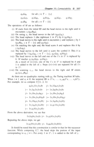
![338 ~ Theory ofComputer Science
Thus we have shown that the three initial primitive recursive functions are
Turing-computable. Next we construct Turing machines that can perform
composition, recursion. and minimization.
11 .4.7 CONSTRUCTION OF THE TURING MACHINE THAT
CAN PERFORM COMPOSITION
Let fIC-'l' X.2' ..., .,,)•...• fiJxI, .... XIII) be Turing-computable functions. Let
g(YI' .. " YI.) be Turing-computable. Let h("I, ..., XIII) =g(fl(XI ...• xm) .•••
.MXi' . , ., XIII»' We construct a Turing machine that can compute h(aj, ...• am)
for given arguments aj, .... am' This involves the following steps:
Step 1 Construct Turing machines All' .... Mk which can compute fl' ..., .I;.
respectively. For the TMs Mj, .... lvII.:' let T' = {I, b, Xl. X.:;• .... xn , y} and
X = 1°1,] 10m
X in by. But the number of states for these TMs will vary.
Let 111 + 1. 11k + 1 be the number of states for /.11, .... A'h. respectively.
As usuaL the initial state is (jo and the states for Mi are qQ, ..., q,,;, As in the
earlier constructions. the set Pi of quadruples for Mi is constructed in such a
way that there is no quadruple starting with ql1;'
Step 2 Let f;(ai' ..., am) = bi for i = 1. 2, ..., k. At the end of step 1,
we have M;'s and the computed values bi's. As g is Turing-computable. we
can construct a TM A'h+l which can compute g(b] • .... bk)· For Mk+l •
X, - Ihl .' 10m ' l .- X ••• X III 7)
(Ve use different markers for Mk+ 1 so that the TM computing h to be
constructed need not scan the inputs a] . ..., am') Let I1k+ + 1 be the number
of states of Mk+]. As in the earlier constructions, Mk+ 1 has no quadruples
starting with qk+ I'
Step 3 At the end of step 2. we have TMs M I , ..., Mb lvh+1 which give
bl ..... bin and g(b] . .... bJ = c (say). respectively. So we are able to
compute h(al' .... am) using k + 1 Turing machines. Our objective is to
construct a single TM kh+.2 which can compute heal' ..., an,). We outline the
construction of M without giving the complete details of the encoding
mechanism. For M. let
T' = {1. b, Xi' " .. X"I' x'.
(1) In the beginning, lv! simulates Mj • As a result. the value bj =
fi(al' ..., am) is obtained as output. Thus we get the tape expression
1°xI 1!!2x.:; ... 1(1mxmlbl y which is the same as that obtained by M1
while halting. lv! does not halt but cbanges y to x'] and adds by to the
right of X'I' The head moves to the left to reach the beginning of X.](https://image.slidesharecdn.com/automata-150510143406-lva1-app6891/85/Automata-351-320.jpg)
![Chapter 11: Computability J;;t 339
(ii) The tape expression obtained at the end of (i) is
The construction given in (i) is repeated. i.e. M simulates M2• .•.• Mk,
changes y to x;, and adds by to the right of x;. After simulating Mk>
the tape expression is
X' = I"IXl ... I"mxm 1btx'l ... 1bk-lXk_tlbkx'k by
Then the head moves to the left until it is positioned at the cell having
1 just to the right of xm.
(iii) M simulates Mk+1• Mk+1 with initial tape expression X' halts with the
tape expression Iblx'i ... Ibkx;" 1'y. As a result, the corresponding tape
expression for M is obtained as
·1"1.- I"2x 1"",.- 1b1 ,J Ibh-' Ii'v.,1 2' . . "", AI'" ., k ~
(iv) The required value is obtained to the left of y. but Ib
tx'l ... Ihkx'k also
appears to the left of c. M erases all these symbols and moves Iiy just
to the right of XIII' The head moves to the cell having x", and M halts.
The final tape expression is 1"lxJI"2x2 ... 1"mxm I(y.
11.4.8 CONSTRUCTION OF THE TURING MACHINE THAT
CAN PERFORM RECURSION
Let g(XI' .... x",). h(Yl' 1'2, .... Ym.d be Turing-computable. Let f(x[o ...,
Xm+1) be defined by recursion as follows:
f(XI' .... Xm • 0) = g(x] ... XII,)
f(x) . ..., x"', I' + 1) = h(xio ..., xm, y, f(xJ' ..., Xm' Y»
For the Turing machine Ai, computing f(a1o .... am, c), (say k), X IS
taken as
As the construction is similar to the construction for computing
composition. ve outline below the steps of the construction.
Step 1 Let l'vf simulate the Turing machine M' which computes g(at, ..., am)'
The computed value, namely g(a) , all,). is placed to the left of y. If
c = O. then the computed yalue g(a] , a,/i) is f(a]- .... am, 0). The head
is placed to the right of Xl/! and M halts.
Step 2 If c is not equal to zero, lito the left of Xm+1 is replaced by bi. The
marker Y is changed to Xm+2 and bv is added to the right of X",+2' The head
moves to the left of 1"1.
Step 3 h is computable. M is allowed to compute h for the arguments at •...,
a",_ O. g(at . ..., am) vhich appear to the left of XJ' ... , xm' Xm+1o XII/+2,](https://image.slidesharecdn.com/automata-150510143406-lva1-app6891/85/Automata-352-320.jpg)
![340 'I Theory of Computer Science
respectively. The computed value is f(a J •••• , 0.1/1' 1). And f(a], ..., 0.1/1' 2)
... f(a], .. " am. c) are computed successively by replacing the rightmost b
and computing h for the respective arguments.
The computation stops with a terminal ill. namely
bI"!>-I'" q··I'·y Ik,. k f( (C')-'I -... .t AI/+] ." =. a], ... , [m'
11.4.9 CONSTRUCTION OF THE TURING MACHINE THAT
CAN PERFORM MINIMIZATION
When f(x], ..., xm) is defined from g(x] . .. " X"1' y) by minimization,
f(xj . .... XI/) is the least of all k's such that g(xlo .... Xm' k) =O. So the
problem reduces to computing g(aj . .... 0.111' k) for given arguments
a), ..., am and for values of k starting from O. f(aj, ..., am) is the first k
for which g(a], .... 0.111' k) = O. Hence as soon as the computed value of
g(a] . .... am' y) is zero, the required Turing machine M has to halt. Of
course, when no such y exists. M never halts, andf(a), ...• am) is not defined.
Thus the construction of M is in such a way that it simulates the TM that
computes g(a] . .... alii' k) for successive values of k. Once the computed value
g(al' .... am' k) =afor the first time. M erases by and changes xlll+I to y. The
head moves to the left of :r,n and M halts.
As partial recursive functions are obtained from the initial functions by a
finite number of applications of composition. recursion and minimization
(Definition 11.11) by the various constructions we have made in this section.
the partial recursive functions become Turing-computable.
Using Godel numbering vhich converts operations of Turing machines
into numeric quantities. it can be proved that Turing-computable functions are
partial recursive. (For proof. refer Mendelson (1964).)
11.5 SUPPLEMENTARY EXAMPLES
EXAMPLE 11.1 3
Shmv that the function f(x), x~, ..., Xli) = 4 IS primitive recursive.
Solution
4 = 5"+(0)
= 5"Z('YtJ)
= 5"+(Z(Uj'(x. x~. ..., XII»)
I.e.
f(x]. X~, .... XII) = S"+(Z( U{'(Xj, X~, ..., xl/)))'
As f is the composition of initial functions, f is primitive recursive.](https://image.slidesharecdn.com/automata-150510143406-lva1-app6891/85/Automata-353-320.jpg)

![344 i;1. Theory ofComputer Science
gif x> v
(f) L(x. ,) =
if x :S y
(1 if x = v
(g) Eer, v) =
to if x *- v
11.3 Compute A(3, 2). A(2, 3), A(3, 3).
11.4 Show that the following functions are primitive recursive:
(a) q(x. y) = the quotient obtained when x is divided by y
(b) rex, y) = the remainder obtained when x is divided by y
{
2X if x is a perfect square
(c) f(x) =
2x + 1 otherwise
11.5 Show that f(x) = integral part of j; is patti'll recursive.
11.6 Show that the Fibonacci numbers are generated by a primitive recursive
function.
11.7 Let f(O) = 1, f(l) = 2, f(2) = 3 and f(x + 3) =f(x) + f(x + 1)1 +
fi.'( + 2)3. Shovv that f(:r) is primitive recursive.
11.8 The characteristic function XA of a given set A is defined as
ra if a ~ A
x(a) = ~
II if a E A
If A, B are subsets of Nand XAo XB are recursive, show that X/, XAuB,
Xv.. B are also recursive.
11.9 Show that the characteristic function of the set of all even numbers is
recursive. Prove that the characteristic function of the set of all odd
integers is recursive.
11.10 Show that the function lex. .1') = x - v is partial recursive.
11.11 Show that a constant function over N. i.e. fen) =k for all n in N where
k is a fixed number. is primitive recursive.
11.12 Show that the characteristic function of a finite subset of N is primitive
recurSIve.
11.13 Show that the addition function fl (x, y) is Turing-computable.
(Represent x and v in tally notation and use concatenation.)
11.14 Show that the Tming machine 1'v1 in the Post notation (i.e. the transition
function specified by quadruples) can be simulated by a Turing
machine Iv! (as defined in Chapter 9).
[Hint: The transition given by a quadruple can be simulated by two
quintuples of i'v1' by adding new states to M~]](https://image.slidesharecdn.com/automata-150510143406-lva1-app6891/85/Automata-357-320.jpg)
![348 ];I Theory of Computer Science
Corollary The order of a polynomial is detennined by its degree.
Defmition 12.2 An exponential function is a function q : N -'7 N defined by
q(n) = a" for some fixed a > 1.
When n increases, each of n, n". 2" increases. But a comparison of these
functions for specific values of 11 will indicate the vast difference between the
growth rate of these functions.
TABLE 12.1 Growth Rate of Polynomial and Exponential Functions
n fen) =n2
g(n) =n2
+ 3n + 9 q(n) =2"
1 1 13 2
5 25 49 32
10 100 139 1024
50 2500 2659 (113)1015
100 10000 10309 (1.27)1030
1000 1000000 1003009 (1.07)10301
From Table 12.1. it is easy to see that the function q(ll) grows at a very fast
rate when compared to fen) or g(ll). In particular the exponential function
grows at a very fast rate when compared to any polynomial of large degree.
We prove a precise statement comparing the growth rate of polynomials and
exponential function.
Deftnition 12.3 We say g '* O(j), if for any constant C and No, there exists
n :2: No such that g(l1) > Cf(n).
Definition 12.4 If f and g are two functions and f = O(g), but g '* O(f),
we say that the growth rate of g is greater than that of.f (In this case
g(n)/f(n) becomes unbounded as 11 increases to 00.)
Theorem 12.2 The growth rate of any exponential function is greater than
that of any polynomial.
Proof Let pen) =ae/ + ak-lnk-1 + . , . + a1n + ao and q(n) = a" for some
a > 1.
As the growth rate of any polynomial is determined by its term with the
highest power, it is enough to prove that Ilk = O(a") and a" '* O(ll), By
L'Hospital's rule. log 11 tends to 0 as n -'7 00. (Here log n = 10gel1.) If
n
then.
I
(~(n»" = le
(log n 'I
As 11 gets large, k ~-'-l-) tends to 0 and hence ~(Il) tends to O.](https://image.slidesharecdn.com/automata-150510143406-lva1-app6891/85/Automata-361-320.jpg)
![is unbounded for large
Chapter 12: Complexity &;! 349
So we can choose No such that ::;(n) ::; a for all n 2: No. Hence n' =
::;(n)" ::; all, proving It' = Oed').
To prove a" i= O(n'), it is enough to show that a"hl is unbounded for
large n. But we have proved that n' ::; a" for large n and any positive integer
a"
k and hence for k + 1. SO ,/+J ::; d' or t:+l:::: 1.
n
Multiplying by n, n (~) 2: n, which means a~nk+l n
values of 11. I
Note: The function n1og " lies between any polynomial function and d 1
for
any constant a. As log n 2: k for a given constant k and large values of n,
nJog " ;:: 11' for large values of n. Hence nJog 11 dominates any polynomial. But
100 Joo , 1 . 1 1 I' (log x)2 B L"H '1'n ,,11= (eJog ,,) "I =e(Jog"f.Letuscacuate 1m . y . ospnas
x~O) ex
. (logx)2 I' 21 lIx I' 210gx l' 2 0
rule, 11m = 1m( ogx)- = 1m --- = 1m - = .
x~o: ex x~o: e X~O: ex X~O: ex
So (log n)2 grows more slowly than en. Hence I1
Jog " = e{]og 11)2 grows more
slowly than 2'''. The same holds good when logarithm is taken over base 2
since logell and lOg211 differ by a constant factor.
Hence there exist functions lying between polynomials and exponential
functions.
12.2 THE CLASSES P AND NP
In this section we introduce the classes P and l'Ii"'P of languages.
Definition 12.5 A Turing machine M is said to be of time complexity T(n)
if the following holds: Given an input 11' of length n. M halts after making at
most T(n) moves.
Note: In this case. lH eventually halts. Recall that the standard TM is called
a deterministic TM.
Definition 12.6 A language L is in class P if there exists some polynomial
T(n) such that L = TUI1) for some deterministic TM M of time complexity
T(n).
EXAMPLE 12.2
Construct the time complexity T(n) for the Turing machine M gIven in
Example 9,7.](https://image.slidesharecdn.com/automata-150510143406-lva1-app6891/85/Automata-362-320.jpg)
![Chapter 12: Complexity f;;! 351
We have seen that a deterministic TM i'vJI simulating a nondetenninistic
TM At exists (refer to Theorem 9.3). If T(n) is the complexity of M, then the
complexity of the equivalent deterministic TM M I is 2°!TIII)). This can be
justified as follows. The processing of an input string w of length n by M is
equivalent to a ·tree' of computations by M j • Let k be the maximum of the
number of choices forced by the nondeterministic transition function. (It is
maxlo(q, .1.')1, the maximum taken over all states q and all tape symbol K)
Every branch of the computation tree has a length T(n) or less. Hence the total
number of leaves is atmost kT(n). Hence the complexity of M I is at most
20ITII/I)
It is not known whether the complexity of M] is less than 2°([(11)). Once
again an answer to this question will prove or disprove P 1= NP. But there do
exist algorithms where T(n) lies between a polynomial and an exponential
function (refer to Section 12.1).
12.3 POLYNOMIAL TIME REDUCTION AND
NP-COMPLETENESS
If P j and P~ are tvo problems and P~ EO P, then we can decide whether
Pi EO P by relating the tVO problems P j and P~. If there is an algorithm for
obtaining an instance of P~ given any instance of Pj, then we can decide about
the problem Pj' Intuitively if this algOlithm is a polynomial one, then the
problem PI can be decided in polynomial time.
DefInition 12.8 Let PI and P~ be two problems. A reduction from PI to P~
is an algorithm which converts an instance of PI to an instance of P~. If the
time taken by the algOlithm is a polynomial pen), n being the length of the
input of Pj. then the reduction is called a polynomial reduction PI to P~.
Theorem 12.3 If there is a polynomial time reduction from Pj to P: and if
P: is in P then Pj is in P.
Proof Let In denote the size of the input of PI' As there is a polynomial-
time reduction of Pj to P:. the corresponding instance of P~ can be got in
polynomial-time. Let it be O(;1'zi), So the size of the resulting input of P: is
atmost Cln! for some constant c. As P~ is in P. the time taken for deciding the
membership in P: is O(ni:} n being the size of the input of P:. So the total
time taken for deciding the membership of m-size input of PI is the sum of
the time taken for conversion into an instance of p, and the time for decision
of the corresponding input in P~. This is O[mi + (cmjll which is the same
as o(mfk). So PI is in P.
Definition 12.9 Let L be a language or problem in NP. Then L is NP-
complete if
1. L is in NP](https://image.slidesharecdn.com/automata-150510143406-lva1-app6891/85/Automata-364-320.jpg)


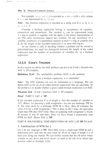
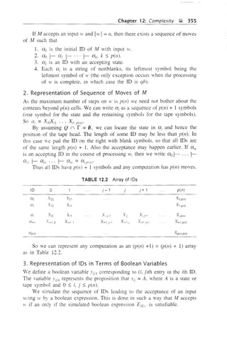
![356 l;! Theory of Computer Science
4. Polynomial Reduction of M to SAT
In order to check that the reduction of M to SAT is correct. we have to ensure
the correctness of
(a) the initial ID.
eb) the accepting ID. and
(c) the intermediate moves between successive IDs,
(al Simulation of initial ID
Xoo must start with the initial state qo of M followed by the symbols of
H' = ala: ' .. all of length n and ending with b's (blank symbol). The
cOlTesponding boolean expression S is defined as
S = )'00'10 i )'Ola; / )'O]a, / ... / )'Olla" / YO,II+1-I) / . .. / YO'P(III,b
Thus given an encoding of M and 1V, we can write S in a tape of a multiple
TM M t, This takes O(p(n)) time,
(b) Simulation of accepting ID
a')II" is the accepting ID. If Pi, P:. . , ., P, are the accepting states of M, then
~Ji'" contains one of Pi' s. 1 :S i :S k in any place j. If al'ill! contains an accepting
state Pi in jth position. then is the accepting state Pi' The corresponding
boolean expression covering all the cases (0 :S j :S pen), 1 :S i :S k) is given
by
F =Fo V F] v .. , V Fpinl
where
F· -,- v 1', V ... v
Each Fi has k variables and hence has constant number of symbols
depending on M but not on n. The number of F;'s in F is pen). Thus given
an encoding of M and H, F can be V11tten in O(p(n)) time on the multiple
TMMI ,
(c) Simulation of intermediate moves
We have to simulate valid moves a i r ai+], i = 0, 1, 2, '" pen).
COlTesponding to each move. ve have to define a boolean variable Ni. Hence
the entire sequence of IDs leading to acceptance of w is
N = No / Nt / ... / NpiliH
First of all note that the symbol X i+Lj can be determined from Xi,j-lo Xij,
Xi.)+] by the move (if there is one changing ai to a different ai+i)' For every
position (i, j). we have t70 cases:
Case 1 The state of ai is at position j.
Case 2 The state of ai is not in any of the (j - l)th, jth and (j + l)th
positions.](https://image.slidesharecdn.com/automata-150510143406-lva1-app6891/85/Automata-369-320.jpg)
![Chapter 12: Complexity ~ 357
Case 1 is taken care of by a variable Ai} and Case 2 by a variable Bu.
The variable Ni will be designed in such a way that it gurantees that ID
(X,+] is one of the IDs that follows the ID (Xi'
X i+l,j can be determined from
(i) the three symbols Xi,j_], Xi). Xi,I+] above it
(ii) the move chosen by the nondeterministic TM M when one of the three
symbols (in (i» is a state.
If the state of (Xi is not Xij, X i.j- 1 or X i.j+l • then Xi+],j = XU, This is taken
care of by the variable BU'
If Xu is the state of (Xi, then X i.I+1 is being scanned by the state Xu' The
move corresponding to the state-tape symbol pair (Xu' X i.i +]) will determine
the sequence X i+1•i - 1 Xi+l. j Xi+1,j+!' This is taken care of by the variable Au'
We write Ni =Ai (Aii v BIi), where A is taken over all is, 0 :::: j :::: pen).
(i) Formulation of Bij When the state of (Xi is none of Xi.i- b Xli' Xi.j +].
then the transition corresponding to (Xi r-- ai+l will not affect X i.i +l • In this
case Xi+l,i = Xij
Denote the tape symbols by ZI' Z:, ..., Z,. Then Xi,i-I' Xi,i and Xi,i+]
are the only tape symbols. So we ""Tite Bii as
Bij =(Yi.i-1. Zl V Yi.i-1. Z2 V ." V Yi.}-1. z) A
V Yi.j+1. z) A
C'i,i, Zl A Zj) V Z2 A Yi+l.j,Z2 V '" V (Yi,j.z,. A Yi+J,j,Z)
This first line of Bij says that Xi. H is one of the tape symbols
ZI_ Z:, . , ., Zj" The second and third lines are regarding Xi.
i and Xi.
i+]. The
fourth line says that Xli and Xi,j+1 are the same and the common value is any
one of Zj_ Z:. ..., Zj"
Recall that the head of M never moves to the left of O-cell and does not
have to move to the right of the p(n)-cell. So Bio will not have the first line
and Bi. jJlil will not have the third line.
(ii) Formulation of Ai} This step corresponds to the correctness of
the 2 x 3 array (see Table 12.3).
TABLE 12.3 Valid Computation
'I- - - - - , - - - - - - - - , . - - - - - - 1
I Xi )-l X f j , xi )+' I
~--- - - - - i - - - 1
!X,r+1,j-1 Xi+1,.) xi+1 ,j+11](https://image.slidesharecdn.com/automata-150510143406-lva1-app6891/85/Automata-370-320.jpg)
![358 J;;i Theory ofComputer Science
The expression B
U
takes care of the case when the state of (Xi is not at the
position X i.j - I , X i.j or X i.j +!. The AU cOlTesponds to the case when the state
of (Xi is at the position Xi)' In this case we have to assign boolean variables
to six positions given in Table 12.3 so that the transition conesponding to
(Xi ~ (Xi+1 is described by the variables in the box correctly.
We say that that an assignment of symbols to the six variables in the box
IS valid if
1. Xu is a state but X i.j _1 and X i.j +! are tape symbols.
2. Exactly one of X i+ l .j- b Xi+l,j, Xi+l. j +i is a state.
3. There is a move which explains how (Xi.j _l , XU, Xi,j+l) changes to
(Xi+1.j-l, Xi+l,j, X i+1.j+l) in (Xi ~ (Xi+!'
There are only a finite number of valid assignments and AU is obtained
by applying OR (that is v) to these valid assignments. A valid assignment
conesponds to one of the fol1owing four cases:
Case A
Case B
Case C
Case D
(p, C, L) E O(q, A)
(p. C, R) E O(q, A)
(Xi =(Xi+! (when (Xi and (Xi"-l contain an accepting state)
j = 0 and j =pen)
Case A Let D be some tape symbol of Ai. Then Xi.j-1XijXi,j+1 = DqA and
X i+1. i-IXi+ Li X i+Li+ 1 =pDC. This can be expressed by the boolean variable.
Yi.j-I, D ; Yi.j. '/ / Yi,j+L / Yi+J.j-l.p / Yi+l.j. D / Yi+Lj+L C
Case B As in case A, let D be any tape symbol. In this case Xi j-1XUXi,j+ I
= DqA and Xi-. i-lXi+1 ,jXi+1.j+l = DCp. The corresponding boolean
expression is
D / q / )'i/+1.-1 / "i+J.!-J.D / Yi+J.j,C / Yi+l,j+J.p
Case C In this case Xij-1XUXi]+1 = Xi"-Li-lXi+l.jXi+l.j+I'
In this case the same tape symbol say D appears in Xi,j-J and Xi+Lj- i ; some
other tape symbol say D ' in X i.j +1 and X i+1.j+I' Xi,j and Xi+!,j contain the
same state. One typical boolean expression is
)'i,j-LZ,. / "i.j.'! / "i,]+J.Zi / Yi+l.j-LZk / Yi+Lj,'! / Yi+Lj+I'zi
Case D Vhen j = 0, we have only X!C0il and Xi+l. 0 Xi+J. I' This is a special
case of Case B. j = pen) conesponds to a special case of Case A.
So. Aii is defined as the OR of all valid telTTIS obtained in Case A to
Case D.
(iii) Definition of N i and N We define Ni and N by
N i = (A iO v B iO) / (Ail v B il ) / ... / (Ai. Pill) V B i,
N = / NI / No / , .. / NpIllJ-1](https://image.slidesharecdn.com/automata-150510143406-lva1-app6891/85/Automata-371-320.jpg)
![Chapter 12: Complexity ~ 359
(iv) Time taken for writing N The time taken to write Bii is a constant
depending on the number Ir I of tape symbols. (Actually the number of
variables in BU is SI r I). The time taken to write AU depends only on the
number of moves of M. As N; is obtained by applying OR to AU / Bij,
o::; i ::; pen) - L 0 ::; j ::; pen) - 1, the time taken to write on Ni is O(p(n».
As N is obtained by applying / to No, Nj, .. " Nl;ll1l~j' the time taken to write
N is p(n)O(p(n» = O(p~(n). .
5. Completion of Proof
Let EM. H = S / N / F.
We have seen that the time taken to write Sand Fare O(p(n» and the
time taken for N is O(p~(n», Hence the time taken to write Elf." is O(p~(n».
Also M accepts ]V if and only if EAt.! is satisfiable.
Hence the deterministic multitape TM Mj can convert w to a boolean
expression EM. II in O(p~(n» time~ An equivalent single tape TM takes
01/'(11» time. This proves the Part II of the Cook's theorem. thus completing
the proof of this theorem. I
12.6 OTHER NP-COMPLETE PROBLEMS
In the last section, we proved the NP-completeness of SAT. Actually it is
difficult to prove the NP-completeness of any problem. But after getting one
NP-complete problem such as SAT. ve can prove the NP-completeness of
problem P' by obtaining a polynomial reduction of SAT to P'. The
polynomial reduction of SAT to P' is relatively easy. In this section we give
a list of NP-complete problems without proving their NP-completeness. Many
of the NP-complete problems are of practical interest.
1. CSAT-Given a boolean expression in Cp,r (conjunctive normal
form-Definition 1.10), is it satisfiable?
We can prove that CSAT is NP-complete by proving that CSAT is
in NP and getting a polynomial reduction from SAT to CSAT,
'1 Hamiltonian circuit problem--Does G have a Hamiltonian circuit (i.e.
a circuit passing through each edge of G exactly once)?
3. Travelling salesman problem (TSP)-Given n cities, the distance
between them and a number D, does there exist a tour programme for
a salesman to visit all the cities exactly once so that the distance
travelled is at most D?
4. Vertex cover problem-Given a graph G and a natural number k, does
there exist a vertex cover for G with k vertices? (A subsets C of
vertices of G is a veltex cover for G if each edge of G has an odd
vertex in C.)](https://image.slidesharecdn.com/automata-150510143406-lva1-app6891/85/Automata-372-320.jpg)

![Chapter 12: Complexity );! 361
12.8.1 QUANTUM COMPUTERS
We know that a bit (a 0 or a 1) is the fundamental concept of classical
computation and information. Also a classical computer is built from an
electronic circuit containing wires and logical gates. Let us study quantum bits
and quantum circuits which are analogous to bits and (classical) circuits.
A quantum bit, or simply qubit can be described mathematically as
Ilf/) = alO; + 1310)
The qubit can be explained as follows. A classical bit has two states, a °and
a 1. Two possible states for a qubit are the states 10; and 11). (The notation
I-l is due to Dirac.) Unlike a classical bit, a qubit can be in infinite number
of states other than 10) and 11). It can be in a state IVJ> =alO) + 1310), where
a and 13 are complex numbers such that lal2
+ 11312
= 1. The 0 and 1are called
the computational basis states and IVJ> is called a superposition. We can call
Ilf/) = alO) + 1310) a quantum state.
In the classical case, we can observe it as a 0 or a 1. But it is not possible
to determine the quantum state on observation. When we measure/observe a
qubit we get either the state 10; with probability lal2
or the state 11) with
probability 11312.
This is difficult to visualize. using our 'classical thinking' but this is the
source of power of the quantum computation.
Multiple qubits can be defined in a similar way. For example. a two-qubit
system has four computational basis states, 100), 1°1), 110; and Ill) and
quantum states Ilf/) = O'{)oIOO) + aodOl) + aiOlI0) + a11I11) with 10'{)o12 + lo:od2
+ la101
2
+ lal112
= l.
Now we define the qubit gates. The classical NOT gate interchanges 0
and 1. In the case of the qubit the NOT gate, a 10) + 1311), is changed to
al1) + 1310;.
The action of the qubit NOT gate is linear on two-dimensional complex
vector spaces. So the qubit NOT gate can be described by
lal~[O 1]la]=[13]
L13J 1 °l13 a
The matrix [~ ~] is a unitary matrix. (A matrix A is unitary if A adjA = I.)
We have seen earlier that {NOR} is functionally complete (refer to
Exercises of Chapter 1). The qubit gate conesponding to NOR is the
cLntrolled-NOT or CNOT gate. It can be described by
IA. B) -7 IA. B EB A)](https://image.slidesharecdn.com/automata-150510143406-lva1-app6891/85/Automata-374-320.jpg)
![362 g Theorv of Computer Science
where EB denotes addition modulo 2. The action on computational basis is
100) ~ 100). 101) ~ 101). 110) ~ Ill), Ill) ~ 110). It can be described by
the following 4 x 4 unitary matrix:
1
° °
~I° 1
°u cx
° ° °
° ° 1 OJ
Now. we are in a position to define a quantum computer:
A quantum computer is a system built from quantllm circuits, contaznmg
wires and elementary quantum gates, to carry out manipulation of quantum
il(foJ7natiol/.
12.8.2 CHURCH-TURING THESIS
Since 1970s many techniques for controHing the single quantum systems have
been developed but with only modest success. But an experimental prototype
for performing quantum cryptography. even at the initial level may be useful
for some real-world applications.
Recall the Church-Turing thesis which asserts that any algorithm that can
be performed on any computing machine can be performed on a Turing
machine as well.
NIiniaturization of chips has increased the power of the computer. The
grmvth of computer power is now described by Moore's law. which states that
the computer power will double for constant cost once in every two years.
Now it is felt that a limit to this doubling power will be reached in two or
three decades. since the quantum effects will begin to interfere in the
functioning of electronic devices as they are made smaller and smaller. So
efforts are on to provide a theory of quantum computation vhich wi]]
compensate for the possible failure of the Moore's law.
As an algorithm requiring polynomial time was considered as an efficient
algorithm. a strengthened version of the Church-TUling thesis was enunciated.
Any algorithmic process can be simulated efficiently by a Turing machine.
But a challenge to the strong Cburch-Turing thesis arose from analog
computation. Certain types of analog computers solved some problems
efficiently whereas these problems had no efficient solution on a TUling
machine. But when the presence of noise was taken into account, the power
of the analog computers disappeared.
In mid-1970s. Robert Soiovay and Volker Strassen gave a randomized
algorithm for testing the primality of a number. (A deterministic polynomial
algorithm was given by Manindra Agrawal. Neeraj Kayal and Nitein Saxena
of IIT Kanpur in 2003.) This led to the modification of the Church thesis.](https://image.slidesharecdn.com/automata-150510143406-lva1-app6891/85/Automata-375-320.jpg)
![366 ~ Theory ofComputer Science
EXAMPLE 12.5
Show that P is closed under (a) union, (b) concatenation, and (c) comple-
mentation.
Solution
Let L j and L2 be two languages in P. Let w be an input of length n.
(a) To test whether W E L j U L2, we test whether W E L j • This takes
polynomial time pen). If W eo L b test another W E L2. This takes
polynomial time q(n). The total time taken for testing whether
W E L j U L2 is pen) + q(n), which is also a polynomial in n. Hence
L j U L2 E P.
(b) Let w =xIX2 •.. x//, For each k, 1 ::; k ::; n - 1, test whether XjX2 •.• Xk
E L j and Xk+jXk+2 ... X/1 E L2• If this happens, W E L jL2. If the test
fails for all k, W eo Lj L2• The time taken for this test for a particular
k is pen) + q(n), where pen) and q(n) are polynomials in n. Hence the
total time for testing for all k's is at most n times the polynomial
pen) + q(n). As n(pn) + q(n) is a polynomial, L]L2 E P.
(c) Let M be the polynomial time TM for Lt. We construct a new TM
AIj as follows:
1. Each accepting state of M is a nonaccepting state of Mj from
which there are no further moves. So if M accepts w, M] on
reading W will halt without accepting.
2. Let qf be a nev state. which is the accepting state of Mj • If
O(q, a) is not defined in M, define 0,11
(q. a) = (qji a, R). So,
W e: L if and only if M accepts wand halts. Also Mj is a
polynomial-time TM. Hence L{ E P.
EXAMPLE 12.6
Show that every language accepted by a standard TM M is also accepted by
a TM lvl] with the following conditions:
1. Mj ' s head never moves to the left of its initial position.
2. M j will never write a blank.
Solution
It is easy to implement Condition 2 on the new machine. For the new TM,
create a new blank b'. If the blank is written by M, the new Turing machine
writes b'. The move of this new TM on seeing b' is the same as the move of
M for b. The new TM satisfies the Condition 2. Denote the modified TM by
M itself. Define the modified M by
M = (Q. 2:. r, 0, q2, b, F)
Define a new TM M j as
M j = (Qj. 2: x {b}, r i • OJ, qQ, [b, bJ, F j )](https://image.slidesharecdn.com/automata-150510143406-lva1-app6891/85/Automata-379-320.jpg)
![Chapter 12: Complexity !;I, 367
where
QI = {qo, qd u (Q x {U. L})
Ij = (I x n u {[x, *] Ix E n
qo and ql are used to initiate the initial move of M. The two-way infinite tape
of M is divided into two tracks as in Table 12.4. Here * is the marker for the
leftmost cell of the lower track. The state [q, U] denotes that M 1 simulates M
on the upper track. [q, L] dentoes that Mj simulates M on the lower track. If
M moves to the left of the cell with *, M 1 moves to the right of the lower
track.
TABLE 12.4 Folded Two-way Tape
Xo X1 X2 II
* K..1 K..2 K.:J
i
I
We can define F 1 of M j by
F1 =F x {U, L}
We can describe D as follows:
1. Dj(qo, [a, bJ) = (qj, [a. *], R)
D(qj. [X, bJ) = ([q:, U], [X, b], L)
By Rule 1, M j marks the leftmost cell in the lower track with * and
initiates the initial move of M.
2. If D(q, X) =(p, Y, D) and 2 E r. then:
(i) D1([q, [;1, [X, 2]) = ([P, [n [Y, 2], D) and
(ii) Dj([q, L], [2, X]) = ([P, L], [2, Y], 15)
where 15 = L if D = Rand 15 = R if D = L.
By Rule 2. M 1 simulates the moves of M on the appropriate track. In
(i) the action is on the upper track and 2 on the lower track is not
changed. In (ii) the action is on the lower track and hence the
movement is in the opposite direction 15; the symbol in the upper
track is not changed.
3. If D(q. X) = (p, Y, R) then
Dj([q. L], [X, *J) = D1([q, [;1, [X, *J) = ([P, [;1, [Y, ,,], R)
When M1 see * in the lower track. M moves right and simulates M
on the upper track.
4. If D(q, X) = (p. Y, L), then
D1([q, L], [X, *J) = D1([q, [;1, [X, "J) = ([P. L]. [1', *]. R)
When Mj sees' in the lower track and M's movement is to the left
of the cell of the two-way tape corresponding to the ;, cell in the
lower track. the M's movement is to X_I and the M1's movement is
also to X_I but towards the right. As the tape of M is folded on the](https://image.slidesharecdn.com/automata-150510143406-lva1-app6891/85/Automata-380-320.jpg)
![368 ~ Theory of Computer Science
cell with *. the movement of M to the left of the *' cell is equivalent
to the movement of MI to the right.
M reaches q in F if and only if M] reaches [q, L) or [q, R). Hence
T(M) = T(ivII ).
EXAMPLE 12.7
We can define the 2SAT problem as the satisfiability problem for boolean
expressions written as / of clauses having two or fewer variables. Show that
2SAT is in P.
Solution
Let the boolean expression E be an instance of the 2SAT problem having 11
variables.
Step 1 Let E have clauses consisting of a single variable (xi or x;). If (x;)
appears as a clause in E, then Xi has to be assigned the truth value T in order
to make E satisfiable. Assign the truth value T to Xi' Once Xi has the truth value
T, then (Xi V)) has the truth value T irrespective of the truth value of 'Yi (Note
that Xi can also be x). So (.I:i V x) or (Xi v x) can be deleted from E. If
E contains (x i V as a clause, then xi should be assigned the truth value T
in order to make E satisfiable. Hence we replace (Xi v Xi) by xi in E so that
.,> should be assigned the truth value T is order to make E satisfiable. Hence
we replace (x i V x) by ."li in E so that xi can be assigned the truth value T
later. If we repeat this process of eliminating clauses with a single variable (or
its negation). we end up in tvo cases.
Case 1 We end up with (Xi) / (x J In this case E is not satisfiable for any
assignment of truth values. We stop.
Case 2 In this case all clauses of E have two variables. (A typical clause is
xi v Xi or Xi v X
Step 2 We have the apply step 2 only in Case 2 of step 1. We have already
assigned truth values for variables not appealing in the reduced expression E.
Choose one of the remaining variables appearing in E. If we have chosen Xi,
assign the truth value T to Xi' Delete ''Ci v Xj or Xi v xi from E. If xi V Xj
appears in E, delete xi to get (Yi)' Repeat step 1 for clauses consisting of a
single variable. If Case 1 occurs. assign the truth value F for Xi and proceed
with E that ve had before applying step 1.
Proceeding with these iterations, we end up either in unsatisfiability of E
or satisfiability of E.
Step 2 consists of repetition of step 1 at most 11 times and step 1 requires
0(11) basic steps.](https://image.slidesharecdn.com/automata-150510143406-lva1-app6891/85/Automata-381-320.jpg)


![380 ;;!. Solutions (or Hints) to Chapter-end Exercises
2.12 Suppose f(x) :::: fey). Then eLY :::: ay. So, x :::: y. Therefore, f is one-one.
f is not onto as any string with b as the first symbol cannot be written
as f(x) for any x E {a, b} *.
2.14 (a) Tree given in Fig. 2.9.
2.15 (a) Yes.
(b) 4. 5. 6 and 8
(c) L 2, 3 and 7
(d) 3 (The longest path is 1 -7 3 -7 7 -7 8)
(e) 4-5-6-8
(f) 2
(g) 6 and 7
2.16 Form a graph G whose vertices are persons. There is an edge
connecting A and B if A knows B. Apply Theorem 2.3 to graph G.
2.17 Proof is by induction on IXI. When IXI :::: L Xis a singleton. Then
2x :::: {0. X}. There is basis for induction. Assume !2X
I :::: 21X1 when
X has 11 - 1 ·elements. Let Y :::: {aj. a~, ..., an}
Y:::: X U {a"L where X:::: {al' a~, ., .. an-d. Then X has 11 - 1
elements. As X has 11 - 1 elements. !2Xj :::: 2[X] by induction hypothesis.
Take any subset Y1 of Y. Either YI is a subset of X or YI - {an}
is a subset of X. So each subset of Y gives rise to two subsets of X.
Thus. !2 Y
:::: 2!2xl. But 12X
:::: i X
. Hence !2Y
:::: 2[Yi. By induction the
result is true for all sets X.
2.18 Ca) When /1 :::: L 1~:::: 1(1 + 1)(1 + 2) :::: L Thus there is basis for
6
induction. Assume the result for 11 - 1. Then
n-l
:::: I k~ -+- 11~
k=1
::::
(11 - 1)(/1 - 1 + 1)(211 - 1) ~
6 +11 [by induction hypothesis]
11(11 + 1)(2/1 + 2) . . . .
:::: 6 on slmphflCatlOn.
Thus the result is true for 11.
(cl When 11 :::: 2, lo~n - 1 :::: 9999 which is divisible by 11. Thus
there is basis for induction. Assume lO~(n-l) - 1 is divisible by 11.
Then, lO~n - 1 :::: lO~lO~(n - I) - 1 :::: 1O~[10~(n - 1) - 1] + 10~ - L As
1O~' 11-1, - 1 and 10~ - 1 are divisible by 11, 1O~" - 1 is divisible by
11. Thus the result is true for 11.](https://image.slidesharecdn.com/automata-150510143406-lva1-app6891/85/Automata-392-320.jpg)
![Solutions (or Hints) to Chapter-end Exercises );1 381
2.19 (b) 22
> 2 [Basis for induction]. Assume 2" - ] > n - 1 for n > 2.
Then. 2" = 2 . 2" - I > 2(n - 1), i.e. 2" > n + n - 2 > n (since
n > 2). The result is true for n. By the principle of induction, the
result is true for all n > 1.
2.20 (a) When n = 1, F(2n + 1) = F(3) = F(l) + F(2) = F(O) + F(2). So,
I
F(2n + 1) = L F(2k).
k=O
Thus there is basis for induction. Assume
,,-1
F(2n - 1) = L F(2k)
k=O
F(2n + 1) =F(2n - 1) + F(2n)
By induction hypothesis,
[by induction hypothesis]
[by definition]
n--l
F(2n + 1) = L F(2k) + F(2n) =
k=O
So the result is true for n.
"
L F(2k)
k=O
2.21 In a simple graph, any edge connects two distinct nodes. The
number of ways of choosing two nodes out of n given nodes is
"e = nell -1) . So the maximum number of edges in a simple graph
- 2
n(n-l)
IS
2
2.22
2.23
We prove by induction on Iwl. When w= A, we have abA = Aab.
Clearly, IAI = 0, which is even. Thus there is basis for induction.
Assume the result for all wwith Iwl < n. Let wbe of length nand
abw = wab. As abw = wab, w = abw] for some w in {a, b}*. So
ababw] = abw]ab and hence abw] = w]ab. By induction hypothesis,
IwI! is even. As Iwl = Iwd + 2, Iwl is also even. Hence by the principle
of induction, the result is true for all w.
Let pen) be the 'open the nth envelope'. As the person opens the first
envelope, P(l) is true. Assume Pen - 1) is true. Then the person
follows the instruction contained therein. So the nth envelope is
opened, i.e. pen) is true. By induction, Pen) is true for all n.
Cnapter 3
3.1 101101 and 000000 are accepted by M. 11111 is not accepted hy M.
3.2 {qo, q], q4}' Now. 8(qo, 010) = {qo, qJ and so 010 is not accepted
by M.](https://image.slidesharecdn.com/automata-150510143406-lva1-app6891/85/Automata-393-320.jpg)
![382 .;!, Solutions (or Hints) to Chapter-end Exercises
3.3 Both the strings are not accepted by M.
3.4 As b(q!, a) = b(q[, a), R is reflexive. Obviously it is symmetric.
If q!Rq2, then b(q[, a) = b(q2, a).
If q2Rq3 then b(q2' a) =b(q3, a). Thus b(q[, a) =b(q3' a), implying
that q!Rq3' So R is an equivalence relation.
3.5 The state table of NDFA accepting {ab, ba} is defined by Table A3.1.
TABLE A3.1 State Table for Exercise 3.5
StatelI. a b
The state table of the corresponding DFA is defined by Table A3.2.
TABLE A3.2 State Table of DFA for Exercise 3.5
StatelI.
[qo]
[q1]
[q2]
~
o
a b
3.6 The NDFA accepting the given set of strings is described by
Fig. A3.1. The corresponding state table is defined by Table A3.3.
a, b
Fig. A3.1 NDFA for Exercise 3.6.
TABLE A3.3 State Table for Exercise 3.6
State/I. a b
qo qo- q1 qo
q1 q2
q2 q3
q3
The DFA accepting the given set is defined by Table A3.4.](https://image.slidesharecdn.com/automata-150510143406-lva1-app6891/85/Automata-394-320.jpg)
![Solutions (or Hints) to Chapter-end Exercises J,;iJ, 383
TABLE A3.4 State Table of DFA for Exercise 3.6
State/I. a b
[qQ] [qQ, q1] [q1]
[qQ, q1] [qQ, q1] [qQ, q2]
[qQ, q2] [qQ, q1, q3] [qoJ
[qQ, q1, q3] [qQ, q1] [qQ, q2]
3.7 The state table for the required DFA is defined by Table A3.5.
TABLEA3.5 State Table for Exercise 3.7
State
[qQ]
[q4]
[q1' q4]
[q2, q3]
o
o 2
[q2, q3]
o
o
[q2' q3]
o
3.9 The state table for the required DFA is defined by Table A3.6.
TABLE A3.6 State Table for Exercise 3.9
State
[q1]
[q2. q3]
[q1' q2]
[q1. q2, q3]
o
[q2, q3]
[q1. q2]
[q1, q2, q3]
[q1, q2, q3]
[q1]
[q1, q2]
[q1]
[q1, q2]
3.10 The required transition system is given in Fig. A3.2. Let L denote
{a, b, c, ..., z}. * denotes any symbol in L - {c, r}. ** denotes any
symbol in L - {c, a, r}. *** denotes any symbol in L.
c
Fig. A3.2 Transition system for Exercise 3.10
3.11 The corresponding Mealy machine is defined by Table A3.7.](https://image.slidesharecdn.com/automata-150510143406-lva1-app6891/85/Automata-395-320.jpg)
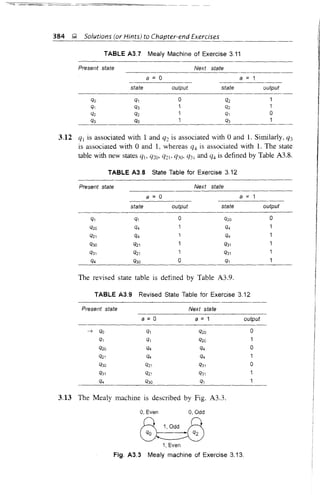


![Solutions (or Hints) to Chapter-end Exercises &,;l, 389
4.17 Let the given granm1ar be Gj . The production A ~ xB where
x =ala2 ... all is replaced by A ~ alAj, Al ~ a2A2, ..., An-I ~
allB. The production A ~ y, where y =blb2 ... bm is replaced by
A ~ bjB], B j ~ b2B2, •••, B/1/-1 ~ b/1/' The grammar G2 whose
productions are the new productions is regular and equivalent to Gj .
Chapter 5
5.1 (a) 0 + 1 + 2
(b) 1(11)*
(c) w in the given set has only one a which can occur anywhere in
w. So w =xay, where x and y consist of some b's (or none).
Hence the given set is represented by b* ab*.
(d) Here we have three cases: w contains no a, one a or two a's.
Arguing as in (c), the required regular expression is
b* + b* ab* + b* ab* ab*
(e) aa(aaa)*
(0 (aa)* + (aaa)* + aaaaa
(g) a(a + b)* a
5.2 (a) The strings of length at most 4 in (ab + a)* are A, a, ab, aa,
aab, aba, abab, a:;, aaba, aaab and d+. The strings in aa + bare
aa and b. Concatenating (i) strings of length at most 3 from the
first set and aa and (ii) strings of length 4 and b, we get the
required strings. They are aa, aaa, abaa, aaaa, aabaa, abaaa,
as, ababb, aabab, aaabb, and aaaab.
(c) The strings in (ab + a) + (ab + a)2 are a, ab, aa, abab, aab and
aha. The strings of length 5 or less in (ab + a)3 are a
3
, abaa,
aaab, ababa. The strings of length 5 or less in (ab + a)4 are a4
,
a3
ab, aba3
• In (ab + a)5, as is the only string of length 5 or less.
The strings in a* are in (ab + a)* as well. Hence the required
strings are A, a, ab, a2, abab, aab, aba, a3
, abaa, aaab, ababa,
a4
, aaaab, abaaa, and as.
5.3 (a) The set of all strings starting with a and ending in abo
(b) The strings are either strings of a's followed by one b or strings
of b's followed by one a.
(c) The set of all strings of the form vw where a's occur in pairs in
v and b's occur in pairs in w.
5.5 The transition system equivalent to (ab + a)*(aa + b) (5.2(a» is
given in Fig. AS.l.](https://image.slidesharecdn.com/automata-150510143406-lva1-app6891/85/Automata-401-320.jpg)

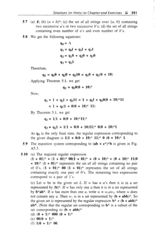

![Solutions (or Hints) to Chapter-end Exercises J;i 393
TABLE A5.1 State Table of DFA for Exercise 5.12
StatelI 0
[qol
[qo, q" q3]
[qo, q2]
[qo, q" Q3, q4]
[qo, q" q3, q,]
[qo, q2, qs]
[qo, q" q3J
[qo, q" q3, q4]
[qo, q" q3, or]
[qo, q" q3, q4]
[qo, q" q3, q4]
[qo, q" q3, qr]
[qo]
[qo, q2]
[qo]
[qo, q2, as]
[qo, q2]
lao]
5.13 Similar to Exercise 3.10.
5.14 The state table for the NDFA accepting (a + b)* abb is defined by
Table A5.2.
TABLE A5.2 State Table for Exercise 5.14
StatelI a b
The corresponding DFA is defined by Table A5.3.
TABLE A5.3 State Table of DFA for Exercise 5.14
StatelI a b
lao] [qo, q,] [qo]
[ao, q,] [qo, q,] [qo, a2]
lao, q2] [00, q,] [qo, qr]
[qo, qr] [qo, q,] [qo, qr]
5.15 Let L be the set of all palindromes over {a, b}. Suppose it is accepted
by a finite automaton M = (Q, L, 8, q, F). {8(qo, a") in 2: I} is a
subset of Q and hence finite. So 8(qo, a") = 8(qo, alll) for some
m and n, m < n. As a"b2"a" E L, 8(qo, a"b2"d') E F. But 8(qo, alll)
= 8(Qo, a"). Hence 8(qo, alllb2"a") = 8(qo, al
b2"a/), which means
alllb2ll
a" E L. This is a contradiction since alllb2
"a" is not a palindrome
(remember m < n). Hence L is not accepted by a finite automaton.
5.16 The proof is by contradiction. Let L = {d'b" In > O}. {8(qo, a") I
n 2 O} is a subset of Q and hence finite. So 8(qo, a") = 8(qo, a1/})
for some m and n, m i= n. So 8(qo, alllb") = 8(8(qo, alll), b") =
8(8(qo, a"), b") = 8(qo, a"b/). As a"b" E L, 8(qo, a"b/) is a final state
and so is 8(qo, a'"b"). This means alllb" E L with m i= n. which is a
contradiction. Hence L is not regular](https://image.slidesharecdn.com/automata-150510143406-lva1-app6891/85/Automata-405-320.jpg)
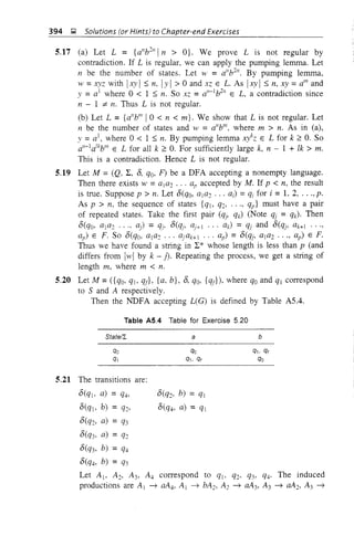
![Solutions (or Hints) to Chapter-end Exercises J; 395
bA4, A4 ~ bA3 (corresponding to the first six transitions) and A2 ~
bAj, A2 ~ b, A4 ~ aAJ, A4 ~ a (corresponding to the last two
transitions). So G = ({Aj, A2, A3, A4 }, {a, b}, P, A j), where P
consists of the induced productions given above.
5.22 The required productions are:
S ~ ASjlBSjl .,. IZSJ,
SI ~ ASI!BSjl '" IZSj,
SI ~ OSlllSI! ... 19S1
Sj ~ AIBI ... IZ and Sj ~ 0[11 '" 19
5.24 The given grammar is equivalent to G =({S, A, B}, {a, b}, P, S),
where P consists of S ~ as IbS IaA, A ~ bB, B ~ a(B ~ aC and
C ~ A is replaced by B ~ a). Let qo, qj and q2 correspond to S, A
and B. qf is the only final state. The transition system M accepting
I(G) is given as
M = ({qo, qj, q2' qf}, {a, b}, 8, qo, {qr})
where qo, qj, and q2 correspond to S, A and Band qf is the (only)
final state. S ~ as, S ~ bS, S ~ aA and A ~ bB induce transitions
from qo to qo with, labels b and a, from qo ~ qj with label a and
from qj to q2 with label b. B ~ a induces a transition from q2 to qf
with label a. M is defined by Fig. AS.5.
a, b
Fig AS.S Transition system for Exercise 5.24.
The equivalent DFA is given in Table AS.S.
TABLE AS.S State Table of DFA for Exercise 5.24
State/I. a b
[qQ] [qQ, q1] [qQl
[qQ, q1] [qQ, q1] [qQ, q2]
[qQ, q2] [qQ. q1. qf] [qQ]
[qQ, q1, qf] [qQ. q1] [qQ. q2]](https://image.slidesharecdn.com/automata-150510143406-lva1-app6891/85/Automata-407-320.jpg)

![398 g Solutions (or Hints) to Chapter-end Exercises
Step 3 We eliminate unit productions. We then have
W(S) = {S} W(A) = {A], WeE) = {E} Wo(B) = {B},
W](B) = {B} u {C}, W2{B) = {B, C} u {D},
W3(B) = {B, C, D, E} = W(B) , W(e) = {C, D, E}, WeD) = {D, E}.
The productions in the new grammar G3 are S ~ AB, A ~ a,
B ~ b, B ~ a and E ~ a. G3 contains the redundant symbol E. So
G3 is not the equivalent grammar in the most simplified form.
6.12 (a) As there are no null productions or unit productions, we can
proceed to step 2.
Step 2 Let GI = (V;y, {O, I}, Pj, S), where PI and V;v are
constructed as follows:
(i) A ~ 0, B ~ 1 are included in Pj.
(ii) S ~ lA, B ~ IS give rise to S ~ CIA, B ~ CIS and CI ~ 1.
(iii) S ~ OB, A ~ OS give rise to S ~ CoB, A ~ CaS and Co ~ 0.
(iv) A ~ lAA, B ~ OBB give rise to A ~ ClAA and B ~ CoBB.
V~y = {S, A, B, Co' Cd.
Step 3 G2 = (Vil, [0. I}, P2, 5), where P2 and v,~, are constructed
as follows:
(i) A ~ 0, B ~ 1, S ~ CIA, B ~ CjS, Cj ~ 1, S ~ CoB,
A ~ CaS, Co ~ °are included in P2•
(ii) A ~ ClAA and B ~ CoBB are replaced by A ~ CIDj, D1 ~
AA, B ~ CoD2' D2 ~ BB.
Thus, G2 = ({S, A, B, Co, Cj, Dj. D 2 }, {O, I}, P2, S) is in CNF and
equivalent to the given grammar where P2 consists of S ~ CjAICoB,
A ~ O!CoS!CIDj, B ~ 1ICISICoD2, CI ~ 1, Co ~ 0, DI ~ AA and
D2 ~ BB.
(b) Step 2 GI = (V'x, {a, b, C}, Pj, S), where PI and V'N are
defined as follows:
(i) S ~ a, S ~ b are included in PI
(ii) S ~ cSS is replaced by S ~ CSS, C ~ c, V",v = {S, C}
Step 3 G2 = (V,<:, {a, b, C}, P2, S). where P2 is defined as follows:
(i) S ~ a, S ~ b, C ~ C are included in P2•
(ii) S ~ CSS is replaced by S ~ CD and D ~ SS.
Thus, the equivalent grammar in CNF is G2 =({S, C, D}, {a, b, c},
P2, S). where P2 consists of S ~ albl CD, C ---;} c, D ---;} SS.
6.13 Consider G =({S}, {a. b, +, *}, P, S), where P consists of S ---;} S + S,
S ---;} S * S. S ~ a, S ~ b.
Step 2 GI = (V(, {a, b, +, 8}, P lo S), where P j is constructed as
follows:
(i) S ~ a, S ~ b are included in PI,
(ii) S ~ S + Sand S ~ S * S are replaced by S ~ SAS, S ~ SBS,
A ~ +, B ~ *
V~· = {S, A, B}](https://image.slidesharecdn.com/automata-150510143406-lva1-app6891/85/Automata-410-320.jpg)
![Solutions (or Hints) to Chapter-end Exercises g 399
Step 3 G: = (~<:, {a, b, +, *}. P:, S), where P2 is constructed as
follows:
(i) S ~ a, S ~ b, A ~ + and B ~ * are included in P2•
(ii) S ~ SAS and S ~ SBS give rise to S ~ SA b A j ~ AS,
S ~ SBj. Bj ~ BS.
The required grammar in CNF is
G2 = ({S, A, B, Aj, Bd, {a, b, +, *}. Pb S)
where P2 consists of
S ~ alblSAdSBj, A ~ +, B ~ *, A j ~ AS and Bj ~ BS
6.14 (a) Rename S as Aj, By Remark following Theorem 6.9, it is enough
to replace terminals by new variables to get an equivalent grammar
Gj. Now, Gj is defined as
Gj = ({A j, A2, A3}, {O, I}, Pb A j)
where Pj consists of
A j ~ AjAIiA2AjA3IA2A3' A2 ~ 0 and A3 ~ 1
This completes step 1.
Step 2 All productions of Gj except A j ~ A jAj are in proper form.
Applying Lemma 6.2 to A j ~ AjA]> we get a new variable Zj and
new productions A j ~ A2A jA3Z j l A2A3Zj, Zj ~ Aj, Zj ~ AjZj • The
new grammar IS
G2 = ({A b A2, A3, Zd, {a, b}, P2, A j)
where P: consists of
A j ~ A2AjA31A2A31A2AtA3ZjlA2A3Zj
Zj ~ AjZj, Zj ~ A j, A2 ~ 0 and Aj ~ 1
Step 3 As A3-productions and Arproductions are in proper form we
have to modify only the A j-productions using Lemma 6.1. So the
modified A j-productions are
A j ~ OA jA31 OA310AjA3ZjlOA3Zj
Step 4 The productions Zj ~ A j and Zj ~ A jZj are modified using
Lemma 6.1. They are:
Zj ~ OA jA31 OA31 OA jA3Z j l OA3Z j
Zj ~ OA jA3Z j IOA3Zj I OA jA3Z jZ j IOA3ZjZj
Thus the required equivalent grammar in GNF is
G3 = ({A j• A:> A3• Zd. {O, I}. P3, A j). where Pj consists of
A j ~ OA j A31 OA31 OA j A3Zj lOA3Z j
A, ~ 0, A3 ~ 1
Zj ~ OA j A31 OA31OA jA3Z j I OA3Z j
Zj ~ OA jA3Z j IOA3Z j IOA j A3Z jZ j IOA3ZjZj](https://image.slidesharecdn.com/automata-150510143406-lva1-app6891/85/Automata-411-320.jpg)


![402 &;l, Solutions (or Hints) to Chapter-end Exercises
production by S ---+ aSBj , B[ ---+ b. (Note: In this problem we can also
replace S ---+ aSb by S ---+ aSB alone. B ---+ b is already in the grammar
and there are no other B-productions.)
(d) The given language is generated by a grammar whose productions
are S ---+ aSb, S ---+ cS. S ---+ c. The equivalent grammar in GNP is
G = ({S, B}, {a, b, c}, P, S),
where P consists of S ---+ aSB, B ---+ b, S ---+ cS, S ---+ c.
6.18 (i) Let W E L(G) and Iwl =k. In the Chomsky normal form, each
production yields one terminal or two variables but nothing else. For
getting the terminals in w, we have to apply production of the form
A ---+ a (k times). The corresponding string of variables, which is of
length k, can be obtained by k - 1 steps. (Each production A ---+ Be
increases the number of variables by one.) So the total number of
steps is 2k - 1. (The reader is advised to prove this result by induction
on Iwl.)
(ii) When G is in GNP, the number of steps in the derivation of w
is k(k = Iwl). The number of terminals increases by 1 for each
application of a production to a sentential form. Hence the number of
steps in the derivation of l-V is k.
6.19 Step 1 Let 11 be the natural number obtained by applying pumping
lemma.
Step 2 Let .:: = a"
2
• Write.:: = UVl-V.xy where 1 ~ Ivxl ~ 11. (This is
possible since Ivwxl ~ n by (ii) of pumping lemma.) Let Ivxl =m,
m ~ n. By pumping lemma, uv2
wx2
y is in L. As luv
2
wx2
yl > n
2
,
IUV2
HX
2
yl = k, where k ;:: n + 1. But luv
2
wx
2
yl = n
2
+ m < n
2
+
2n + 1. So luv2w~yI strictly lies between n2 and (n + 1)2 which means
uv2
wx2
y E L. a contradiction. Hence {a"
2
: n;:: I} is not context-free.
6.20 (a) Take.:: =d'b"c" in L(G). Write z =UVw,xy, where 1 ~ Ivxl ~ n.
So vx cannot contain all the three symbols a, band c. So uv2
wx2
y
contain additional occurrences of two symbols (found in vx) and the
number of occurrences of the third symbol remains the same. This
means the number of occurrences of the three symbols in UV
2
WX
2
y are
not the same and so uv2w~y E L. This is a co~tradiction. Henc~ the
language is not context-free.
(b) As usual, n is the integer obtained from pumping lemma.
Let z = d'b"c21
. Then z = uV],VX)', where 1 ~ Ivxl ~ n. So vx cannot
contain all the three symbols a, band c. If vx contains only a's and
b's then we can choose i such that uviwxiy has more than 2n
occurrences of a (or b) and exactly 2n occurrences of c. This means
uviwxiy E L, a contradiction. In other cases too, we can get a
contradiction by proper choice of i. Thus the given language is not
context-free.](https://image.slidesharecdn.com/automata-150510143406-lva1-app6891/85/Automata-414-320.jpg)
![Solutions (or Hints)to Chapter-end Exercises ~ 403
6.21 (a) Suppose G = (VN, L, P, S) is right-linear. A production of the
form A ~ a]a2 ... amB, m ~ 2 can be replaced by A ~ alA],
A] ~ a2A2 ..., Am_] ~ amB. A ~ b]b2 ... bm, m ~ 2, can be
replaced by A ~ bIB], B] ~ b2Bb ..., Bm-2 ~ blll_]Bm_], Bm_] ~
bm. The required equivalent regular grammar G' is defined by the new
productions constructed above.
If G =(VN, L, P, S) is left-linear, then an equivalent right-linear
grammar can be defined as G) =(V'N, L, Ph S), where PI consists of
(i) S ~ W when S ~ W is in P and W E L*,
(ii) S ~ wA when A ~ W is in P and W E L*,
(iii) A ~ wB when B ~ Aw is in P and w E L*,
(iv) A ~ w when S ~ Aw is in P and w E L*.
Let w E L(G). If S => w then S ~ w is in P. Therefore, S ~ w is
in PI (by (i».
Assume S => Alwl => A2W2W] => ... Am_1wm_] ... WI => WmWm_1
... WI =W is a derivation in G. Then the productions applied in the
derivation are S ~ Alw], A] ~ A2W2, ..., AIIl- 1 ~ Wm. The induced
productions in G] are
A] ~ WI, A2 ~ W2A h A3 ~ W02, ., ., S ~ wlI,Am-]
(by (ii), (iii) and (iv)' in the construction of PI)'
Taking the productions in the reverse order we get a derivation of G]
as follows:
Thus L(G) ~ L(G'). The other inclusion can be proved in a similar
way. So G is equivalent to a right-linear grammar G] which is
equivalent to a regular grammar.
(b) Let G = ({S, A}, {a, b, e}, P, S). where P consists of S ~
Sc IAc, A ~ aAb lab. G is linear (by the presence of A ~ aAb).
L(G) = {allbl/ellli m, n ~ I}
Using pumping lemma we prove that L(G) is not regular. Let n be the
number of states in a finite automaton accepting L(G).
Let w =a'W'c". By pumping lemma w =xyz, where Ixyl ::; nand
Iy I> O. If y =J< then xz =a"-kYle". This is not in L(G). By pumping
lemma. xz E L(G) a contradiction.
6.22 L =L(G), where G is a regular grammar. For every variable A in G.
A :b ex implies ex =uB, where u E L* and B E V, Thus Gis nonself-
embedding. To prove the sufficiency part, assume that G is a nonself-
embedding, context-free grammar. If G' is reduced, in Greibach
normal form and equivalent to G, then G' is also nonself-embedding.
(This can be proved.) Let IL I =nand m be the maximum of the
lengths of right-hand sides of productions in G'. Let ex be any](https://image.slidesharecdn.com/automata-150510143406-lva1-app6891/85/Automata-415-320.jpg)
![404 g Solutions (or Hints) to Chapter-end Exercises
sentential form. By considering leftmost derivations, we can show that
the number of variables in a is ::; mn. (Use the fact that G/ is in GNF).
Define:
Gl = (Vf:, ~, PI, 5) where
Vf: = {[a]llal ::; mn and a E Vn
51 = [51]
PI = {[Af3] ~ b[a 13] IA ~ ba is in P, 13 E Vf: and laf3l ::; mn}
GI is regular. It can be verified that L(GI ) = L(G').
Chapter 7
7.1 (qo, aacaa, Zo) t- (qo, acaa, aZo) r- (qo, caa, aaZo) r- (qj, a, aaZo)
r- (qjo a, aZo) r- (qj, A, Zo) r- (qj' A, Zo)·
(i) Yes, the final ill is (qr, A, Zo)·
(ii) Yes, the final ill is (qjo A, aZo)·
(iii) No, the pda halts at (ql' ba, aZo)·
(iv) Yes, the final ill is (ql' A, abaZo)
(v) Yes, the final ill is (qo, A, babaZo)·
7.2 (i) (qj, A, aZo).
(ii) Halts at (q), b. A).
(iii) (qo, A, a5
Zo)·
(iv) Does not move.
(v) Does not move.
(vi) Halts at (qjo ab, Zo).
7.3 (a) Example 7.9.
(b) The required pda A is defined as follows:
A = ({qo, ql' q:;}, {a, b}, {a, Zo}, 6, qo, Zo, 0). 6 is defined by
6(qo, a, Zo) = {(ql' aZo)} , 6(ql' a, a) = {(qlo aa)}
6(qlo b, a) = {(q:;, a)}, 6(q:;, b, a) = {(qj, A)}
6(q, A, Zo) = {(qjo A)}.
(c) A = ({qo, qd, {a, b, C}, {Zo, Zd, 6, qo, Zo, 0)
6 is defined by
6(qo, a, Zo) = {(qo, ZIZa)}, 6(qo, a, ZI) = {(qo, ZIZ1)}
6(qo, b, Z) = {(qj, A)}, 6(ql' b, ZI) = {(qlo A)}
6(qlo c, Zo) = {(ql, Za)}, 6(ql' A, Zo) = {(ql' A)}
Note that on reading a, we add ZI; on reading b we remove ZI and
the state is changed. If the input is completely read and the stack
symbol is Zo, then it is removed by a A-move.
7.4 (a) Example 7.9 gives a pda accepting {a"blll
a" 1m, n ~ I} by null
store. Using Theorem 7.1, a pda B accepting the given language by
final state is constructed.](https://image.slidesharecdn.com/automata-150510143406-lva1-app6891/85/Automata-416-320.jpg)
![406 ~ Solutions (or Hints) to Chapter-end Exercises
7.7 (i) Define G = ({S}, {a, b}, P, 5). where P consists of
S ~ SaSbSaS, S ~ SaSaSbS, S ~ SbSaSaS. S ~ A
(Refer to Exercise 4.1O(e).) G is the required grammar. (ii) Apply
Theorem 7.3. (iii) Apply Theorem 7.1 to the pda obtained in (ii).
7.8 Let A =({qo, qd, {a. b}, {Zo. a, b}, 8, qo, Zo, 0). where 8 is given
by
8(qo. a. Zo) = {(qo. aZo)}' 8(qo, b, Zo) = {(qo, bZo)}
8(qo. a. h) = {(qo. ab)}, 8(qo, b. a) = {(qo. ba)}
8(qo, a, a) = {(qo. aa). (q)o A)}
8(qo, b. b) = {(qo. bb), (q, A)}
8(qo, A, Zo) = {(qlo A)}
8(qj. a. a) = {(qjo A)}, 8(qlo b, b) = {(qlo A)}
8(ql. A. Zo) = {(qlo A)}
A makes a guess whether it has reached the centre of the string. A
reaches the centre only when the input symbol and the topmost
symbol on PDS are the same. This explains the definition of
8(qo, a. a) and 8(qo. b. b). A accepts the given set by null store.
7.9 Example 7.6 gives a pda A accepting the given set by empty store.
The only problem is that it is not deterministic. We have 8(q. a, Zo)
= {(q. aZo)} and 8(q. A, Zo) = {(q, A)}. So A is not deterministic
(refer to Definition 7.5). But the construction can be modified as
follows:
Al = ({q. q]}, {a, b}, {Zo. a, b}, 8, q. Zo. 0)
where 8 is defined by the following rules:
8(q. a, Zo) = {(qto aZo)}. 8(q. b. Zo) = {(ql. bZo)}
8(q], a. a) = {(ql, aa)}, 8(ql. b, b) = {(qlo bb)}
8(q]. a, b) = {(qlo A)}, 8(qlo b. a) = {(q]o A)}
8(q]o A, Zo) = {(% A)}
A] is deterministic and accepts the given set by empty store.
7.10 The S-productions are
S ~ [qo. Zo. qo] I [qo, Zo, qJJ
8(q]. b, a) = {(ql. A)}, 8(q]o A, Zo) = {(qlo A)}
and
8(qo, b. a) = {(q]o A)}
Now these induce [qlo a. qJJ ~ b. [q], Zo. ql] ~ A and [qo, a. qd
~ b. respectively. 8(qo, a, Zo) = {(qo, aZo)} induces](https://image.slidesharecdn.com/automata-150510143406-lva1-app6891/85/Automata-418-320.jpg)
![Solutions (or Hints) to Chapter-end Exercises ); 407
[qo, 7-{), qo] ~ a[qo, a, %][qo, Zo, qo]
[qo, Zo, qo] ~ a[qo, a, qJJ[qj, Zo, qo]
[qo, Zo, ql] ~ a[qo, a, qo][qo, Zo, qd
[qo, Zo, qd ~ a[qo, a, qd(qlo Zo, qd
8(qo, a, a) = {(qo, aa)} induces
[qo, a, qo] ~ a[qo, a, qo][qo, a, qo]
[qo,a, qo] ~ a[qo, a, qd(qIo a, qo]
[qo, a, qJJ ~ a[qo, a, qo][qo, a, ql]
[qo, a, qI] ~ a[qo, a, ql][qlo a, qd
7.13 Let M =(Q, L, 8, qo, F) be a DFA accepting a given regular set.
Define a pda A by A =(Q, L, {Zo}. 8Io qo, ~, F). 8 is given by the
following rule:
81(q, a, Zo) = {(qQ, Zo)} if 8(q, a) =q'
It is easy to see that T(M) =T(A). Let w E n~. Then 8(qo, w) =
q' E F.
8(qo, w, Zo) = {(q', Zo)}· So W E T(A), i.e., T(M) C T(A). The
proof that T(A) C T(M) is similar.
7.15 If 8(q, a, z) contains (q', 2122 ... 211), n ~ 3. we introduce new states
qj, q2, ..., qn-2' We define new transitions involving new states as
follows:
(i) (% 211
_ 1211 ) is included in (Kq, a, Z)
(ii) 8(qi, A, ZIl_i) = {(qi+Io 21l- i- 1 2,,_)} for i = 1, 2, ..., n - 3
(iii) 8(q"_2' A, 22) = {(q', 2 122)}
This construction is repeated for every transition given by (q', y) E
8(q, a, 2), IYI ~ 3. Deleting such transitions and adding the new
transitions induced by them we get a pda which never adds more than
one symbol at a time.
Chapter 8
8.1 For a sentential form such as a"+lbll
, A ~ a is the production applied
in the last step only when a is followed by abo So A ~ a is a handle
production if and only if the symbol to the right of a is scanned and
found to be b. Similarly, A ~ aAb is a handle production if and only
if the symbol to the right of aAb is b. Also, S ~ aAb is a handle
production if and only if the symbol to the right of aAb is A.
Therefore, the grammar is LR(l), but not LR(O).
8.2 We can actually show that the given grammar is not LR(k) for any
k ~ O. Suppose it is LR(k) for some k. Consider the rightmost](https://image.slidesharecdn.com/automata-150510143406-lva1-app6891/85/Automata-419-320.jpg)


![Solutions (or Hints) to Chapter-end Exercises Q 411
10.14 Suppose there exists a Turing Machine Mover {O, l} and a state qlll
such that the problem of determining whether or not M will enter qm
is unsolvable. Define a new Turing machine M' which simulates M and
has the additional transition given by 6(qm' A) = (qm' 1, R). Then M
enters qlll when it starts with a given tape configuration if and only if
M' prints 1 when it starts with a given tape configuration. Hence the
given problem is unsolvable.
10.17 According to Church's thesis we can construct a Turing Machine which
can execute any given algorithm. Hence the given statement is false.
(Of course, the Church's thesis is not proved. But there is enough
evidence to justify its acceptance.)
10.18 Let L ={a}. Let x =(x], X2, ..., xn) and Y =(YI, Y2, ..., Yn), where
. - k; • _ 1 2 d }. - Ii . - 12Th ()Il( )IZX, - a , I - , , ..., n an )j - a·, ] - , , ..., n. en Xl X2
.. .(xjlJ =(Yli1(Y2)kZ... (Y,ilJ
• Both are equal to aLkil
;. Hence PCP is
solvable when IL I = 1.
10.20 Xl =01, Y1 =OIl, X2 =1, Y2 = 10, x3 = 1, Y3 =1. Hence IXi I < IYi I
for i = 1, 2, 3. So XilXi2 ... xim :;t. YiIYiz ... Yim for no choice of i's.
Note: IxilXiz ... xlm 1 < 1Yi1Yiz ... Yim I· Hence the PCP with the given
lists has no solution.
10.21 Xl =0, Y1 =10, X2 = 110, Y2 =000, X3 =001, Y3 = 10. Here no pair
(Xlo YI), (x2' Y2) or (x3' Y3) has common nonempty initial substring. So
XilXiz ... xim :;t. YilYiz ... Yim for no choice of i/s. Hence the PCP with
the given lists has solution.
10.22 As Xl =Y1, the PCP with the given lists has a solution.
10.23 In this problem, Xl = 1, X2 = 10, X3 = 1011, Y1 = 111, Y2 = 0,
Y3 = 10. Then, XJX1X1X2 =Y3Y1Y1Y2 = 101111110. Hence the PCP with
the given lists has a solution. Repeating the sequence 3, 1, 1, 2, we can
get more solutions.
10.24 Both (a) and (b) are possible. One of them is possible by Church's
thesis. Find out which one?
Chapter 11
11.1 (a) The function is defined for all natural numbers divisible by 3.
(b) x =2
(c) x ;:: 2
(d) all natural numbers
(e) all natural numbers
11.2 (a) X(Oj(O) = 1, X(Oj(x + 1) -'- X(Ojsgn(p(x»)
(b) f(x + 1) = x2
+ 2x + 1
So, f(x + 1) = f(x) + S(S(Z(x»)) * ui(x) + S(Z(x»](https://image.slidesharecdn.com/automata-150510143406-lva1-app6891/85/Automata-423-320.jpg)


![414 j; Solutions (or Hints) to Chapter-end Exercises
11.15 qo1ll1xlby ~ llllqoXlby ~ llllqlxby. As b lies between Xl and y,
Z(4) =0 (given by b).
11.16 In Section 11.4.5 we obtained q01xlby ~ qs1xbbly. Similarly,
qoll1xlby ~ qs1llxlb1y ~ 1qollxlbly. Proceeding further,
1qollxlb1y ~ 1qsllxlblly ~ llqolxlblly f-"'- lllqc;Xllllly (as in
Section 11.4.5). Hence S(3) = 4.
11.18 Represent the argument x in tally notation. j(x) = S(S(x». Using the
construction given in Section 11.4.7, we can construct a TM which
gives the value S(S(x».
11.19 f(x]> X2) =S(S(U?(x]> X2»)' Use the construction in Section 11.4.7.
11.20 Represent (Xl> X2) by P1bl'2. By taking the input as $1'Ib1'2($ is
representing the left-end) and suitably modifying the TM given in
Example 9.6, we get the value of Xl + X2 to the right of $.
Chapter 12
12.1 Denote j(n)
k
= L aini and g(n) =1=0
I
L bini, where aj, bi' are positive
./=0 <
k
integers. Assume k :2 t. Then fen) + g(n) = L (ai + bJn
i
, where bi = 0
1=0
for i > l. f(n) + g(n) is a polynomial of degree k. Hence j(n)g(n) =
O(nk+/).
12.2 As n2
dominates n log nand n2
10g n dominates n2
, the growth rate of
hen) > growth rate of g(n). Note f(n) =g(n) = 0(n2
).
Jl II 11
12.3 As L i =n(n + 1)/2, L P=n(n + 1)(211 + 1)/6 and L P=(n(n + 1)12)2,
1=0 1=0 1=0
the answers for (i) and (ii) are 0(n3
) and O(n (iii) a(1 - r")/l - r =
n
O(l'lr) = 0(1'-1). (iv) '2 [2a + (n-1)d] = 0(n2
).
12.4 As log2 n, 10g3 n, loge n, differ by a constant factor, j(n) = O(r/ log n)
12.5 gcd =3.
12.6 The principal disjunctive normal form of the boolean expression has
5 terms (refer to Example 1.13). P ; Q ; R is one such term. So
(T, T, T) satisfies the given expression. Similar assignments for the
other four terms.
12.7 No.
12.8 (T. T, F, F) makes the given expression satisfiable.
12.9 Only if: Take an NP-complete problem L. Then r is in CO-NP = NP.](https://image.slidesharecdn.com/automata-150510143406-lva1-app6891/85/Automata-426-320.jpg)


This document is the preface to a textbook on the theory of computer science. It discusses the changes made in the third edition of the book compared to the second edition. Some of the key changes include adding a new chapter on decidability and recursively enumerable languages, expanding the sections on pigeonhole principle and induction, including a proof of Kleene's theorem in regular languages chapter, and adding a new chapter on complexity theory and quantum computation. The preface provides an overview of the topics covered in each chapter and emphasizes that the book includes numerous examples, detailed solutions to exercises, and self-test questions in each chapter to aid student learning.