Multi-layer perceptrons (MLPs) are a type of artificial neural network used in machine learning, characterized by their multiple layers including at least one hidden layer. MLPs are trained using the backpropagation learning algorithm, which adjusts weights based on errors from predicted and actual outputs. They are effective classifiers across various domains, such as optical character recognition and image classification tasks like those involving the MNIST dataset.

1. Sajid Majeed -220380-PhD CyS-III
Muhammad Shahzad-230405 PhD CyS-I
Department of Cyber Security
Air University ,Islamabad
Multi-layer Perceptrons (MLPs)

2. Introduction -What is an MLP?
• Multi-layer perceptrons (MLPs) are a type of
artificial neural network that have been widely
used for various machine learning tasks.
• An MLP is a feedforward neural network that
consists of multiple layers of perceptrons.
• It is called a "multi-layer" network because it
has at least one hidden layer between the
input and output layers.
• A Multilayer Perceptron (MLP) is a fully
connected neural network, i.e., all the nodes
from the current layer are connected to the
next layer.
• A MLP consisting in 3 or more layers: an input
layer, an output layer and one or more hidden
layers.

3. What is an MLP? Cont..
• Perceptrons are the basic building blocks of an MLP.
• They take a set of input values, apply weights to them, and produce an output value
based on an activation function.
• Activation functions are used to introduce non-linearity into the output of the
perceptrons.
• Common activation functions used in MLPs include sigmoid, tanh, and ReLU.
• Forward propagation is the process of passing input data through the network to
produce an output.
• Each layer of perceptrons takes the output of the previous layer and applies weights
and activation functions to produce its own output.
• Backpropagation is the process of adjusting the weights in the network based on
the error between the predicted output and the actual output.
• It uses the chain rule of differentiation to calculate the gradient of the loss function
with respect to the weights in each layer.
4 September 2024

4. Multi-layer Perceptron neural architecture
4 September 2024
• In a typical MLP network, the input units (Xi) are fully
connected to all hidden layer units (Yj) and the hidden layer
units are fully connected to all output layer units (Zk)
• Each of the connections
between the input to hidden
and hidden to output layer
units has an associated weight
attached to it (Wij or Wjk)
• The hidden and output layer
units also derive their bias
values (bj or bk) from
weighted connections to units
whose outputs are always 1
(true neurons)

5. MLP training algorithm
4 September 2024
• A Multi-Layer Perceptron (MLP) neural network trained
using the Backpropagation learning algorithm is one of the
most powerful forms of supervised neural network system.
• MLP utilizes a supervised learning technique called back
propagation for training.
• The training of such a network involves three stages:
• Feedforward of the input training pattern,
• Calculation and backpropagation of the associated error
• Adjustment of the weights
• This procedure is repeated for each pattern over several
complete passes (epochs) through the training set.
• After training, application of the net only involves the
computations of the feedforward phase.

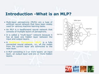
6. Backpropagation Learning Algorithm
4 September 2024
Feed Forward phase:
• Xi = input[i]
• Yj = f( bj + XiWij)
• Zk = f( bk + YjWjk)
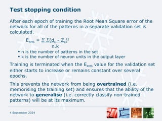
Backpropagation of errors:
• k = Zk[1 - Zk](dk - Zk)
• j = Yj[1 - Yj]  k Wjk
Weight updating:
• Wjk(t+1) = Wjk(t) + kYj + [Wjk(t) - Wjk(t - 1)]
• bk(t+1) = bk(t) + kYtn + [bk(t) - bk(t - 1)]
• Wij(t+1) = Wij(t) + jXi + [Wij(t) - Wij(t - 1)]
• bj(t+1) = bj(t) + jXtn + [bj(t) - bj(t - 1)]

7. Test stopping condition
4 September 2024
After each epoch of training the Root Mean Square error of the
network for all of the patterns in a separate validation set is
calculated.
ERMS =  (dk - Zk)2
n.k
• n is the number of patterns in the set
• k is the number of neuron units in the output layer
Training is terminated when the ERMS value for the validation set
either starts to increase or remains constant over several
epochs.
This prevents the network from being overtrained (i.e.
memorising the training set) and ensures that the ability of the
network to generalise (i.e. correctly classify non-trained
patterns) will be at its maximum.

8. Factors affecting network performance
4 September 2024
Number of hidden nodes:
• Too many and the network may memorise training set
• Too few and the network may not learn the training set
Initial weight set:
• some starting weight sets may lead to a local minimum
• other starting weight sets avoid the local minimum.
Training set:
• must be statistically relevant
• patterns should be presented in random order
Date representation:
• Low level - very large training set might be required
• High level – human expertise required

9. MLP as classifiers
4 September 2024
MLP classifiers are used in a wide range of domains from
engineering to medical diagnosis. A classic example of use
is as an Optical Character Recogniser.
Simple example would be a
35-8-26 mlp network. This
network could learn to map
input patterns, corresponding
to the 5x7 matrix
representations of the capital
letters A - Z, to 1 of 26
output patterns.
After training, this network then classifies ‘noisy’ input
patterns to the correct output pattern that the network
was trained to produce.

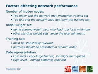
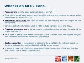
10. Training an MLP on MNIST-Image
Classification
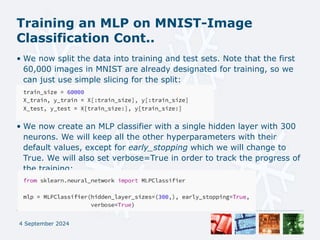
• The data set contains 60,000 training images and 10,000 testing
images of handwritten digits. Each image is 28 × 28 pixels in size,
and is typically represented by a vector of 784 numbers in the range
[0, 255]. The task is to classify these images into one of the ten
digits (0–9).
• We first fetch the MNIST data set using the fetch_openml()
function:
• The as_frame parameter specifies that we want to get the data and
the labels as NumPy arrays instead of DataFrames (the default of
this parameter has changed in Scikit-Learn 0.24 from False to
‘auto’).
4 September 2024

11. Training an MLP on MNIST-Image
Classification Cont..
• Let’s examine the shape of X:
• That is, X consists of 70,000 flat vectors of
784 pixels.
• Let’s display the first 50 digits in the data
set:
4 September 2024

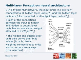
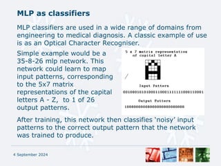
12. Training an MLP on MNIST-Image
Classification Cont..
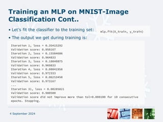
• Let’s check how many samples we have from each digit:
• The data set is fairly balanced between the 10 classes.
• We now scale the inputs to be within the range [0, 1] instead of [0,
255]:
• Feature scaling makes the training of neural networks faster and
prevents them from getting stuck in local optima.
4 September 2024

13. Training an MLP on MNIST-Image
Classification Cont..
• We now split the data into training and test sets. Note that the first
60,000 images in MNIST are already designated for training, so we
can just use simple slicing for the split:
• We now create an MLP classifier with a single hidden layer with 300
neurons. We will keep all the other hyperparameters with their
default values, except for early_stopping which we will change to
True. We will also set verbose=True in order to track the progress of
the training:
4 September 2024

14. Training an MLP on MNIST-Image
Classification Cont..
• Let’s fit the classifier to the training set:
• The output we get during training is:
4 September 2024

15. Training an MLP on MNIST-Image
Classification Cont..
• The training stopped after 31 iterations, since the validation score
has not improved during the previous 10 iterations.
• Let’s check the accuracy of the MLP on the training and the test
sets:
• These are great results, but networks with more complex
architectures such as convolutional neural networks (CNNs) can
achieve even better results on this data set.
4 September 2024

16. Training an MLP on MNIST-Image
Classification Cont..
• To understand better the errors of our
model, let’s display its confusion matrix:
• We can see that the main confusions of the
model are between the digits 4 9, 7 9 and
⇔ ⇔
2 8. This makes sense since these digits
⇔
often resemble each other when written by
hand.
4 September 2024

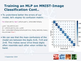
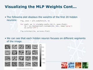
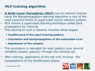
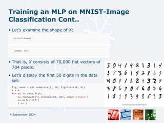
17. Visualizing the MLP Weights
• Although neural networks are generally considered to be “black-box”
models, in simple networks that consist of one or two hidden layers, we
can visualize the learned weights and occasionally gain some insight into
how these networks work internally.
• For example, let’s plot the weights between the input and the hidden
layers of our MLP classifier. The weight matrix has a shape of (784,
300), and is stored in a variable called mlp.coefs_[0]:
• Column i of this matrix represents the weights of the incoming inputs to
hidden neuron i. We can display this column as a 28 × 28 pixel image,
in order to examine which input neurons have a stronger influence on
this neuron’s activation.
4 September 2024

18. Visualizing the MLP Weights Cont...
• The following plot displays the weights of the first 20 hidden
neurons:
• We can see that each hidden neuron focuses on different segments
of the image.
4 September 2024

19. Conclusion
• MLPs are a powerful type of neural network that can be
used for various machine learning tasks.
• Each layer passing its output to the next layer until the
final output is produced.
• The weights of the perceptrons are updated through the
training process to minimize the error between the
predicted output and the actual output.
• The use of multiple hidden layers can improve the
accuracy of the network.
• By understanding their basic structure and workings, we
can better utilize them in our own applications.
4 September 2024