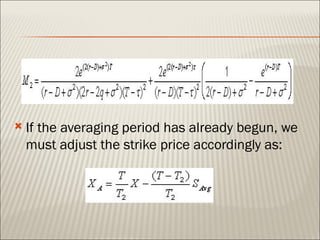
Presented by:
Pooja Singh
N. Krishna
Iyer
   Asian options are options in which the
    underlying variable is the average price over
    a period of time.

   Because of this fact, Asian options have a
    lower volatility and hence rendering them
    cheaper relative to their European
    counterpar ts.
   They are broadly segregated into three
    categories;
       arithmetic average Asians,
        geometric average Asians and
        both these forms can be averaged on a weighted
        average basis, whereby a given weight is applied to each
        stock being averaged.
           E.g.. highly skewed sample population.
   Valuation of Asian options presents problems due to
    the fact that while distribution of stock prices is known
    to be lognormal, the probability distribution of the
    average is unknown.
   Kemna & Vorst (1990) put forward a closed form
    pricing solution to geometric averaging options by
    altering the volatility, and cost of carry term.
    Geometric averaging options can be priced via a
    closed form analytic solution because of the reason
    that the geometric average of the underlying prices
    follows a lognormal distribution as well, whereas with
    arithmetic average rate options, this condition
    collapses.
   The solutions to the geometric averaging
    Asian call and puts are given as:
   Where N(x) is the cumulative normal
    distribution function of:


   which can be simplified to
   The adjusted volatility and dividend yield are
    given as:


   Where is the observed volatility, r is the risk
    free rate of interest and D is the dividend
    yield.
   As there are no closed form solutions to
    arithmetic averages due to the inappropriate
    use of the lognormal assumption under this
    form of averaging, a number of approximations
    have emerged in literature. The approximation
    suggested by Turnbull and Wakeman (TW)
    (1991) makes use of the fact that the
    distribution under arithmetic averaging is
    approximately lognormal, and they put forward
    the first and second moments of the average in
    order to price the option.
   The analytical approximations for a call and a
    put under TW are given as:
 Where T2 is the time remaining until
  maturity. For averaging options which have
  already begun their averaging period, then
  T2 is simply T (the original time to maturity),
  if the averaging period has not yet begun,
  then is T2 is
 The adjusted volatility and dividend yield are
  given as:
   To generalise the equations, we assume that
    the averaging period has not yet begun and
    give the first and second moments as:
   If the averaging period has already begun, we
    must adjust the strike price accordingly as:
   Where we reiterate T as the original time to
    maturity, as the remaining time to maturity, X as
    the original strike price and    is the average
    asset price. Haug (1998) notes that if r = D, the
    formula will not generate a solution.
   http://www.global-
    derivatives.com/index.php/component/content/17?task=view
Asian options

Asian options

  • 1.
  • 2.
    Asian options are options in which the underlying variable is the average price over a period of time.  Because of this fact, Asian options have a lower volatility and hence rendering them cheaper relative to their European counterpar ts.
  • 3.
    They are broadly segregated into three categories;  arithmetic average Asians,  geometric average Asians and  both these forms can be averaged on a weighted average basis, whereby a given weight is applied to each stock being averaged.  E.g.. highly skewed sample population.
  • 4.
    Valuation of Asian options presents problems due to the fact that while distribution of stock prices is known to be lognormal, the probability distribution of the average is unknown.
  • 5.
    Kemna & Vorst (1990) put forward a closed form pricing solution to geometric averaging options by altering the volatility, and cost of carry term. Geometric averaging options can be priced via a closed form analytic solution because of the reason that the geometric average of the underlying prices follows a lognormal distribution as well, whereas with arithmetic average rate options, this condition collapses.
  • 6.
    The solutions to the geometric averaging Asian call and puts are given as:
  • 7.
    Where N(x) is the cumulative normal distribution function of:  which can be simplified to
  • 8.
    The adjusted volatility and dividend yield are given as:  Where is the observed volatility, r is the risk free rate of interest and D is the dividend yield.
  • 9.
    As there are no closed form solutions to arithmetic averages due to the inappropriate use of the lognormal assumption under this form of averaging, a number of approximations have emerged in literature. The approximation suggested by Turnbull and Wakeman (TW) (1991) makes use of the fact that the distribution under arithmetic averaging is approximately lognormal, and they put forward the first and second moments of the average in order to price the option.
  • 10.
    The analytical approximations for a call and a put under TW are given as:
  • 11.
     Where T2is the time remaining until maturity. For averaging options which have already begun their averaging period, then T2 is simply T (the original time to maturity), if the averaging period has not yet begun, then is T2 is  The adjusted volatility and dividend yield are given as:
  • 12.
    To generalise the equations, we assume that the averaging period has not yet begun and give the first and second moments as:
  • 13.
    If the averaging period has already begun, we must adjust the strike price accordingly as:
  • 14.
    Where we reiterate T as the original time to maturity, as the remaining time to maturity, X as the original strike price and is the average asset price. Haug (1998) notes that if r = D, the formula will not generate a solution.
  • 15.
    http://www.global- derivatives.com/index.php/component/content/17?task=view