This presentation lets you know about Apache Mahout. The Apache Mahout is a machine learning library and the main goal is to build scalable machine learning libraries.

1. Mahout

2. What is Machine Learning?
A few things come to mind

3. Really it’s…
―Machine Learning is programming computers
to optimize a performance criterion using
example data or past experience‖

4. Getting Started with ML
Get your data
Decide on your features per your algorithm
Prep the data
Different approaches for different algorithms
Run your algorithm(s)
Lather, rinse, repeat
Validate your results
Smell test, A/B testing, more formal methods

5. Where is ML Used Today
Internet search clustering
Knowledge management systems
Social network mapping
Marketing analytics
Recommendation systems
Log analysis & event filtering
SPAM filtering, fraud detection
And many more ……

6. Mahout

7. What is Mahout
The Apache Mahout™ machine learning library's goal is to
build scalable machine learning libraries.
Mahout currently has
Scalable to reasonably large data
Collaborative Filtering
sets. Our core algorithms for
User and Item based
clustering, classification and batch
recommenders
based collaborative filtering are
K-Means, Fuzzy K-Means clustering
implemented on top of Apache
Mean Shift clustering
Hadoop using the map/reduce
Dirichlet process clustering
paradigm.
Latent Dirichlet Allocation
However Mahout does not restrict
Singular value decomposition
contributions to Hadoop based
Parallel Frequent Pattern mining
implementations:
Complementary Naive Bayes
The core libraries are highly
classifier
optimized to allow for good
Random forest decision tree based
performance also for non-distributed
classifier
algorithms
High performance java collections
(previously colt collections)

8. Why Mahout ?
An Apache Software Foundation project to create scalable
machine learning libraries under the Apache Software License
Many Open Source ML libraries either:
Lack Community
Lack Documentation and Examples
Lack Scalability
Lack the Apache License
Or are research-oriented

9. Focus: Machine Learning
Applications
Examples
Freq.
Classificatio
Genetic Pattern Clustering Recommenders
n
Mining
Math
Utilities Collections Apache
Vectors/Matrice
Lucene/Vectorizer (primitives) Hadoop
s/SVD

10. Focus: Scalable
Goal: Be as fast and efficient as possible
given the intrinsic design of the algorithm
Some algorithms won’t scale to massive machine
clusters
Others fit logically on a Map Reduce framework
like Apache Hadoop
Still others will need alternative distributed
programming models
Be pragmatic
Most Mahout implementations are Map
Reduce enabled
(Always a) Work in Progress

11. Use Cases
Currently Mahout supports mainly three use cases:
Recommendation mining takes users' behaviour and
from that tries to find items users might like.
Clustering takes e.g. text documents and groups
them into groups of topically related documents.
Classification learns from existing categorized
documents what documents of a specific category look
like and is able to assign unlabelled documents to the
(hopefully) correct category.

12. Algorithms and Applications

13. Recommendation
Predict what the user likes based on
His/Her historical behavior
Aggregate behavior of people similar to him

14. Recommender Engines
Recommender engines are the most immediately recognizable
machine learning technique in use today. You’ll have seen services or
sites that attempt to recommend books or movies or articles based
on your past actions. They try to infer tastes and preferences and
identify unknown items that are of interest:
Amazon.com is perhaps the most famous e-commerce site to
deploy recommendations. Based on purchases and site
activity, Amazon recommends books and other items likely to be of
interest.
Netflix similarly recommends DVDs that may be of interest, and
famously offered a $1,000,000 prize to researchers who could
improve the quality of their recommendations.
Dating sites like Líbímseti can even recommend people to people.
Social networking sites like Facebook use variants on
recommender techniques to identify people most likely to be as-
yet-unconnected friends.

15. Mahout Recommenders
Different types of recommenders
User based
Item based
Full framework for storage, online and offline
computation of recommendations
Like clustering, there is a notion of similarity
in users or items
Cosine, Tanimoto, Pearson and LLR

16. User-based recommendation
Have you ever received a CD as a gift? I did, as a youngster, from my
uncle . Uncle once evidently headed down to the local music store and
cornered an employee, where the following scene unfolded:
Now they’ve inferred a similarity based directly on tastes in music.
Because the two kids in question both prefer some of the same bands, it
stands to reason they’ll each like a lot in the rest of each other’s
collections. They’ve actually based their idea of similarity between the two
teenagers on observed tastes in music. This is the essential logic of a user-
based recommender system.

17. Exploring the user-based recommender
for every other user w
compute a similarity s between u and w
retain the top users, ranked by similarity, as a neighborhood n
for every item i that some user in n has a preference for,
but that u has no preference for yet
for every other user v in n that has a preference for i
compute a similarity s between u and v
incorporate v's preference for i, weighted by s, into a running
average
The outer loop simply considers every known user then computes
the most similar users and only items known to those users are considered
in the inner loop. For those items where the user had no preference but
the similar user has some preference .
In the end, the values are averaged to come up with an estimate
weighted average, that is each preference value is weighted in the average
by how similar that user is to the target user. The more similar a user, the
more heavily their preference value is weighted

18. Mahout Recommender Architecture
A Mahout-based collaborative filtering engine takes users'
preferences for items ("tastes") and returns estimated
preferences for other items.
For example, a site that sells books or CDs could easily use
Mahout to figure out, from past purchase data, which CDs a
customer might be interested in listening to.
Mahout provides a rich set of components from which you
can construct a customized recommender system from a
selection of algorithms. Mahout is designed to be enterprise-
ready; it's designed for performance, scalability and flexibility.
Mahout recommenders are not just for Java; it can be run
as an external server which exposes recommendation logic to
your application via web services and HTTP.
Top-level packages define the Mahout interfaces to these
key abstractions:
DataModel
UserSimilarity
ItemSimilarity
UserNeighborhood
Recommender
These are the pieces from which you will build your own
recommendation engine. That's it!
.

19. A simple user-based recommender program
DataModel model = new FileDataModel (new File("intro.csv"));
UserSimilarity similarity = new PearsonCorrelationSimilarity (model);
UserNeighborhood neighborhood =new NearestNUserNeighborhood
(2, similarity, model);
Recommender recommender = new GenericUserBasedRecommender (
model, neighborhood, similarity);
List<RecommendedItem> recommendations = recommender.recommend(1, 1);
for (RecommendedItem recommendation : recommendations) {
System.out.println(recommendation);
}
UserSimilarity encapsulates some notion of similarity among users, and
User-Neighborhood encapsulates some notion of a group of most-similar
users. These are necessary components of the standard user-based
recommender algorithm.

20. Components In Detail
DataModel
A DataModel implementation stores and provides access to all the
preference, user, and item data needed in the computation.
The simplest DataModel implementation available is an in-memory
implementation,GenericDataModel. It’s appropriate when you want to
construct your data representation in memory, programmatically, rather
than base it on an existing external source of data, such as a file or
relational database.
An implementation might draw this data from any source, but a
database is the most likely source. Mahout provides
MySQLJDBCDataModel, for example, to access preference data from a
database via JDBC and MySQL. Another exists for PostgreSQL. Mahout
also provides a FileDataModel.
There are no abstractions for a user or item in the object .Users
and items are identified solely by an ID value in the framework.
Further, this ID value must be numeric; it is a Java long type through the
APIs. A Preference object or PreferenceArray object encapsulates the
relation between user and preferred items

21. Components In Detail …
UserSimilarity
A UserSimilarity defines a notion of similarity between two Users. This is a
crucial part of a recommendation engine. These are attached to a Neighborhood
implementation. ItemSimilarities are analagous, but find similarity between Items.
UserNeighborhood
In a user-based recommender, recommendations are produced by finding a
"neighborhood" of similar users near a given user. A UserNeighborhood defines a
means of determining that neighborhood — for example, nearest 10 users.
Implementations typically need a UserSimilarity to operate.
Recommender
A Recommender is the core abstraction in Mahout. Given a DataModel, it can
produce recommendations. Applications will most likely use the
GenericUserBasedRecommender implementation or the
GenericItemBasedRecommender.

22. Exploring with GroupLens
GroupLens (http://grouplens.org/) is a research project that provides several
data sets of different sizes, each derived from real users’ ratings of movies.
From the GroupLens site, locate and download the ―100K data set,‖ currently
accessible at http://www.grouplens.org/node/73. Unarchive the file you
download, and within find the file called ua.base. This is a tab-delimited file with user
IDs, item IDs, ratings (preference values), and some additional information.
DataModel model = new FileDataModel (new File(―ua.base"));
RecommenderEvaluator evaluator = new
AverageAbsoluteDifferenceRecommenderEvaluator ();
RecommenderBuilder recommenderBuilder = new RecommenderBuilder() {
@Override
public Recommender buildRecommender(DataModel model) throws TasteException
{
UserSimilarity similarity = new PearsonCorrelationSimilarity(model);
UserNeighborhood neighborhood = new
NearestNUserNeighborhood(100, similarity, model);
return new GenericUserBasedRecommender( model, neighborhood, similarity);
}
};
double score = evaluator.evaluate(recommenderBuilder, null, model, 0.95, 0.05);
System.out.println(score);

23. Pearson correlation–based similarity
So far, examples have used the PearsonCorrelationSimilarity implementation,
which is a similarity metric based on the Pearson correlation.
.
The Pearson correlation is a number between –1 and 1 that measures the tendency
of two series of numbers, paired up one-to-one, to move together. That is to say, it
measures how likely a number in one series is to be relatively large when the
corresponding number in the other series is high, and vice versa. It measures the
tendency of the numbers to move together proportionally, such that there’s a
roughly linear relationship between the values in one series and the other. When
this tendency is high, the correlation is close to 1. When there appears to be little
relationship at all, the value is near 0. When there appears to be an opposing
relationship—one series’ numbers are high exactly when the other series’ numbers
are low—the value is near –1

24. Pearson correlation–based similarity
1,101,5.0
1,102,3.0 We noted that users 1 and 5 seem similar because their
1,103,2.5 preferences seem to run together. On items
101, 102, and 103, they roughly agree: 101 is the
2,101,2.0 best, 102 somewhat less good, and 103 isn’t desirable. By
2,102,2.5 the same reasoning, users 1 and 2 aren’t so similar.
2,103,5.0
2,104,2.0
Item 101 Item 102 Item 103 Correlation
with user 1
3,101,2.5
3,104,4.0 User 1 5.0 3.0 2.5 1.000
3,105,4.5
User 2 2.0 2.5 5.0 -0.764
4,101,5.0 User 3 2.5
4,103,3.0
4,104,4.5 User 4 5.0 3.0 1.000
User 5 4.0 3.0 2.0 0.945
5,101,4.0
5,102,3.0
5,103,2.0 The Pearson correlation between user 1 and other users
5,104,4.0 based on the three items that user 1 has in common with
5,105,3.5 the others
Note : A user’s Pearson correlation with itself is always 1.0.

25. Other Similarities in Mahout
The Euclidean Distance Similarity
Euclidian distance is the square root of the sum of the squares of the differences in
coordinates.
Try EuclideanDistanceSimilarity—swap in this implementation by changing the
UserSimilarity implementation to new EuclideanDistanceSimilarity(model) instead.
This implementation is based on the distance between users. This idea makes sense if
you think of users as points in a space of many dimensions (as many dimensions as there
are items), whose coordinates are preference values. This similarity metric computes the
Euclidean distance d between two such user points.
The Cosine Measure Similarity
The cosine measure similarity is another similarity metric that depends on
envisioning user preferences as points in space. Hold in mind the image of user
preferences as points in an n-dimensional space. Now imagine two lines from the origin, or
point (0,0,...,0), to each of these two points. When two users are similar, they’ll have
similar ratings, and so will be relatively close in space—at least, they’ll be in roughly the
same direction from the origin.
The angle formed between these two lines will be relatively small. In
contrast, when the two users are dissimilar, their points will be distant, and likely in
different directions from the origin, forming a wide angle. This angle can be used as the
basis for a similarity metric in the same way that the Euclidean distance was used to form
a similarity metric. In this case, the cosine of the angle leads to a similarity value.

26. Other Similarities in Mahout
Spearman correlation
The Spearman correlation is an interesting variant on the Pearson
correlation, for our purposes. Rather than compute a correlation based on the
original preference values, it computes a correlation based on the relative rank of
preference values. Imagine that, for each user, their least-preferred item’s
preference value is overwritten with a 1. Then the next-least-preferred item’s
preference value is changed to 2, and so on.
To illustrate this, imagine that you were rating movies and gave your least-
preferred movie one star, the next-least favourite two stars, and so on. Then, a
Pearson correlation is computed on the transformed values. This is the Spearman
correlation
Tanimoto Coefficient Similarity
Interestingly, there are also User-Similarity implementations that ignore
preference values entirely. They don’t care whether a user expresses a high or low
preference for an item —only that the user expresses a preference at all. It doesn’t
necessarily hurt to ignore preference values.
TanimotoCoefficientSimilarity is one such implementation, based on the
Tanimoto coefficient. It’s the number of items that two users express some
preference for, divided by the number of items that either user expresses some
preference.
In other words, it’s the ratio of the size of the intersection to the size of the
union of their preferred items. It has the required properties: when two users’
items completely overlap, the result is 1.0. When they have nothing in common, it’s
0.0.

27. Other Recommender

28. Item-based recommendation
Item-based recommendation is derived from how similar items are to items, instead
of users to users. In Mahout, this means they’re based on an ItemSimilarity
implementation instead of UserSimilarity.
Lets look at the CD store scenario again
ADULT: I’m looking for a CD for a teenage boy.
EMPLOYEE: What kind of music or bands does he like?
ADULT: He wears a Bowling In Hades T-shirt all the time and seems to have all of
their albums. Anything else you’d recommend?
EMPLOYEE: Well, about everyone I know that likes Bowling In Hades seems to like the new
Rock Mobster album.
Algorithm
for every item i that u has no preference for yet
for every item j that u has a preference for
compute a similarity s between i and j
add u's preference for j, weighted by s, to a running average
return the top items, ranked by weighted average
Code
public Recommender buildRecommender(DataModel model)
throws TasteException {
ItemSimilarity similarity = new PearsonCorrelationSimilarity(model);
return new GenericItemBasedRecommender(model, similarity);
}

29. Slope-one recommender
It estimates preferences for new items based on average difference in
the preference value (diffs) between a new item and the other items the
user prefers.
The slope-one name comes from the fact that the recommender
algorithm starts with the assumption that there’s some linear relationship
between the preference values for one item and another, that it’s valid to
estimate the preferences for some item Y based on the preferences for
item X, via some linear function like Y = mX + b. Then the slope-one
recommender makes the additional simplifying assumption that m=1: slope
one. It just remains to find b = Y-X, the (average) difference in
preference value, for every pair of items.
And then, the recommendation algorithm looks like this:
for every item i the user u expresses no preference for
for every item j that user u expresses a preference for
find the average preference difference between j and i
add this diff to u's preference value for j
add this to a running average
return the top items, ranked by these averages
You can easily try the slope-one recommender. It takes no similarity
metric as a necessary argument:

30. Distributing Recommendation
Computations

31. Analyzing the Wikipedia Data Set
Wikipedia (http://wikipedia.org) is a well-known online encyclopedia,
whose contents can be edited and maintained by users. It reports that in
May 2010 it contained over 3.2 million articles written in English alone.
The Freebase Wikipedia Extraction project
http://download.freebase.com/wex/) estimates the size of just the English
articles to be about 42 GB. Wikipedia articles can and do link to one
another. It’s these links that are of interest. Think of articles as users,
and the articles that an article points to as items that the source article
likes.
Fortunately, it’s not necessary to download Freebase’s well-organized
Wikipedia extract and parse out all these links. Researcher Henry
Haselgrove has already extracted the article links and published just this
information at http://users.on.net/~henry/home/wikipedia.htm.
This further filters out links to ancillary resources like article discussion
pages, images, and such. This data set has also represented articles by
their numeric IDs rather than titles, which is helpful, because Mahout
treats all users and items as numeric IDs.

32. Constructing a Co-occurrence Matrix
Recall that the item-based implementations so far rely on an ItemSimilarity
implementation, which provides some notion of the degree of similarity between any
pair of items.
Instead of computing the similarity between every pair of items, Lets compute
the number of times each pair of items occurs together in some user’s list of
preferences, in order to fill out the matrix called a co-occurrence matrix .
For instance, if there are 9 users who express some preference for both
items X and Y, then X and Y co-occur 9 times. Two items that never appear together
in any user’s preferences have a co-occurrence of 0
101 102 103
101 5 3 4
102 3 3 3
103 4 3 4
Co-occurrence is like similarity; the more two items turn up together, the more
related or similar they probably are. The co-occurrence matrix plays a role like that
of ItemSimilarity in the nondistributed item-based algorithm.

33. Producing the recommendations
Multiplying the co-occurrence matrix with user 3’s preference vector (U3) to
produce a vector that leads to recommendations, R
101 102 103 U3 R
101 5 3 4 10.0
2.0
102 3 3 3 0.0 6.0
103 4 3 4 0.0 8.0
4(2.0) + 3(0.0) + 4(0.0)
Table shows this multiplication for user 3 in the small example data set, and the
resulting vector R. It’s possible to ignore the values in rows of R corresponding to
items 101 because these aren’t eligible for recommendation.
User 3 already expresses a preference for these items. Of the remaining
items, the entry for item 103 is highest, with a value of 8.0, and would therefore be
the top recommendation, followed by 102 /

34. Towards a distributed implementation
This is all very interesting, but what about this algorithm is more
suitable for large scale distributed implementations?
It’s that the elements of this algorithm each involve only a
subset of all data at any one time. For example, creating user
vectors is merely a matter of collecting all preference values for
one user and constructing a vector. Counting co-occurrences only
requires examining one vector at a time. Computing the resulting
recommendation vector only requires loading one row or column of
the matrix at a time. Further, many elements of the computation
just rely on collecting related data into one place efficiently— for
example, creating user vectors from all the individual preference
values.
The MapReduce paradigm was designed for computations with
exactly these features.

35. Translating to MapReduce: generating user vectors
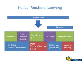
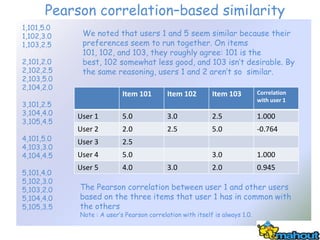
In this case, the computation begins with the links data file as input. Its lines aren’t of
the form userID, itemID, preference. Instead they’re of the form userID: itemID1 itemID2
itemID3 .... This file is placed onto an HDFS instance in order to be available to Hadoop.
The first MapReduce will construct user vectors:
Input files are treated as (Long, String) pairs by the framework, where the Long
key is a position in the file and the String value is the line of the text file. For
example, 239 / 98955: 590 22 9059
Each line is parsed into a user ID and several item IDs by a map function. The
function emits new key-value pairs: a user ID mapped to item ID, for each item
ID. For example, 98955 / 590
The framework collects all item IDs that were mapped to each user ID together.
A reduce function constructors a Vector from all item IDs for the user, and outputs
the user ID mapped to the user’s preference vector. All values in this vector
are 0 or 1. For example, 98955 / [590:1.0, 22:1.0, 9059:1.0]

36. A mapper that parses Wikipedia link files
public class WikipediaToItemPrefsMapper extends
Mapper<LongWritable,Text,VarLongWritable,VarLongWritable> {
private static final Pattern NUMBERS = Pattern.compile("(d+)");
public void map(LongWritable key,Text value,Context context)
throws IOException, InterruptedException {
String line = value.toString();
Matcher m = NUMBERS.matcher(line);
m.find();
VarLongWritable userID = new VarLongWritable(Long.parseLong(m.group()));
VarLongWritable itemID = new VarLongWritable();
while (m.find()) {
itemID.set(Long.parseLong(m.group()));
context.write(userID, itemID);
}
}}

37. Reducer which produces Vectors from a user’s item preferences
public class WikipediaToUserVectorReducer extends
Reducer<VarLongWritable,VarLongWritable,VarLongWritable,Vect
orWritable> {
public void reduce(VarLongWritable userID,
Iterable<VarLongWritable> itemPrefs, Context context)
throws IOException, InterruptedException {
Vector userVector = new RandomAccessSparseVector(
Integer.MAX_VALUE, 100);
for (VarLongWritable itemPref : itemPrefs) {
userVector.set((int)itemPref.get(), 1.0f);
}
context.write(userID, new VectorWritable(userVector));
}
}

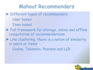
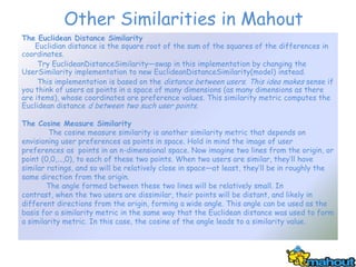
38. Translating to MapReduce: calculating co-occurrence
The next phase of the computation is another MapReduce that uses the output of
the first MapReduce to compute co-occurrences.
1 Input is user IDs mapped to Vectors of user preferences—the output of the last
MapReduce. For example, 98955 / [590:1.0,22:1.0,9059:1.0]
2 The map function determines all co-occurrences from one user’s preferences,
and emits one pair of item IDs for each co-occurrence—item ID mapped to
item ID. Both mappings, from one item ID to the other and vice versa, are
recorded. For example, 590 / 22
3 The framework collects, for each item, all co-occurrences mapped from that
item.
4 The reducer counts, for each item ID, all co-occurrences that it receives and
constructs a new Vector that represents all co-occurrences for one item with a
count of the number of times they have co-occurred. These can be used as the
rows—or columns—of the co-occurrence matrix. For example,
590 / [22:3.0,95:1.0,...,9059:1.0,...]
The output of this phase is in fact the co-occurrence matrix.

39. Mapper component of co-occurrence computation
public class UserVectorToCooccurrenceMapper extends
Mapper<VarLongWritable,VectorWritable,IntWritable,IntWritable> {
public void map(VarLongWritable userID, VectorWritable userVector,
Context context) throws IOException, InterruptedException {
Iterator<Vector.Element> it =
userVector.get().iterateNonZero();
while (it.hasNext()) {
int index1 = it.next().index();
Iterator<Vector.Element> it2 = userVector.get().iterateNonZero();
while (it2.hasNext()) {
int index2 = it2.next().index();
context.write(new IntWritable(index1),
new IntWritable(index2));
}
}
}

40. Reducer component of co-occurrence computation
public class UserVectorToCooccurrenceReducer extends
Reducer<IntWritable,IntWritable,IntWritable,VectorWritable> {
public void reduce(IntWritable itemIndex1,
Iterable<IntWritable> itemIndex2s,
Context context)
throws IOException, InterruptedException {
Vector cooccurrenceRow =
new RandomAccessSparseVector(Integer.MAX_VALUE, 100);
for (IntWritable intWritable : itemIndex2s) {
int itemIndex2 = intWritable.get();
cooccurrenceRow.set(
itemIndex2,
cooccurrenceRow.get(itemIndex2) + 1.0);
}
context.write(
itemIndex1,
new VectorWritable(cooccurrenceRow));
}
}

41. Translating to MapReduce: rethinking matrix multiplication
It’s now possible to use MapReduce to multiply the user vectors computed in step 1,
and the co-occurrence matrix from step 2, to produce a recommendation vector from
which the algorithm can derive recommendations.
But the multiplication will proceed in a different way that’s more efficient here—a
way that more naturally fits the shape of a MapReduce computation. The algorithm
won’t perform conventional matrix multiplication, wherein each row is multiplied
against the user vector (as a column vector), to produce one element in the result R:
for each row i in the co-occurrence matrix
compute dot product of row vector i with the user vector
assign dot product to ith element of R
Why depart from the algorithm we all learned in school? The reason relates purely to
performance, and this is a good opportunity to examine the kind of thinking necessary
to achieve performance at scale when designing large matrix and vector operations.
Instead, note that matrix multiplication can be accomplished as a function of the co-
occurrence matrix columns:
assign R to be the zero vector
for each column i in the co-occurrence matrix
multiply column vector i by the ith element of the user vector
add this vector to R

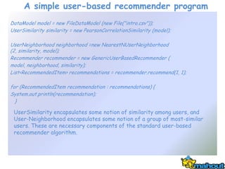
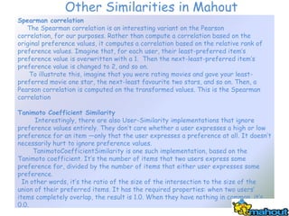
42. Translating to MapReduce: matrix multiplication by partial products
The columns of the co-occurrence matrix are available from an earlier
step. The columns are keyed by item ID, and the algorithm must multiply
each by every nonzero preference value for that item, across all user
vectors. That is, it must map item IDs to a user ID and preference
value, and then collect them together in a reducer. After multiplying the co-
occurrence column by each value, it produces a vector that forms part of
the final recommender vector R for one user.
The mapper phase here will actually contain two mappers, each producing
different
types of reducer input:
Input for mapper 1 is the co-occurrence matrix: item IDs as keys, mapped
to columns as vectors. For example, 590 / [22:3.0,95:1.0,...,9059:1.0,...]
Input for mapper 2 is again the user vectors: user IDs as keys, mapped to
preference Vectors. For example, 98955 / [590:1.0,22:1.0,9059:1.0]
For each nonzero value in the user vector, the map function outputs an
item ID mapped to the user ID and preference value, wrapped in a
VectorOrPref-Writable. For example, 590 / [98955:1.0]
The framework collects together, by item ID, the co-occurrence column and
all user ID–preference value pairs. The reducer collects this information
into one output record and stores it.

43. Wrapping co-occurrence columns
Shows the co-occurrence columns being wrapped in a VectorOr-
PrefWritable.
public class CooccurrenceColumnWrapperMapper extends
Mapper<IntWritable,VectorWritable, IntWritable,VectorOrPrefWritable>
{
public void map(IntWritable key,VectorWritable value,
Context context) throws IOException, InterruptedException {
context.write(key, new VectorOrPrefWritable(value.get()));
}
}

44. Splitting User Vectors
Shows that the user vectors are split into their individual preference values and output, mapped by
item ID rather than user ID.
public class UserVectorSplitterMapper extends Mapper<VarLongWritable,VectorWritable,
IntWritable,VectorOrPrefWritable> {
public void map(VarLongWritable key, VectorWritable value, Context context) throws
IOException, InterruptedException {
long userID = key.get();
Vector userVector = value.get();
Iterator<Vector.Element> it = userVector.iterateNonZero();
IntWritable itemIndexWritable = new IntWritable();
while (it.hasNext()) {
Vector.Element e = it.next();
int itemIndex = e.index();
float preferenceValue = (float) e.get();
itemIndexWritable.set(itemIndex);
context.write(itemIndexWritable,
new VectorOrPrefWritable(userID, preferenceValue));
}
}
}

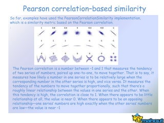
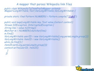
45. Computing partial recommendation vectors
With columns of the co-occurrence matrix and user preferences in hand, both keyed by item
ID, the algorithm proceeds by feeding both into a mapper that will output the product of the
column and the user’s preference, for each given user ID.
1 Input to the mapper is all co-occurrence matrix columns and user preferences
by item. For example, 590 / [22:3.0,95:1.0,...,9059:1.0,...] and 590 /
[98955:1.0]
2 The mapper outputs the co-occurrence column for each associated user times
the preference value. For example, 590 / [22:3.0,95:1.0,...,9059:1.0,...]
3 The framework collects these partial products together, by user.
4 The reducer unpacks this input and sums all the vectors, which gives the user’s
final recommendation vector (call it R). For example, 590 /
[22:4.0,45:3.0,95:11.0,...,9059:1.0,...]
public class PartialMultiplyMapper extends Mapper<IntWritable,VectorAndPrefsWritable,
VarLongWritable,VectorWritable> {
public void map(IntWritable key, VectorAndPrefsWritable vectorAndPrefsWritable, Context context)
throws IOException, InterruptedException {
Vector cooccurrenceColumn = vectorAndPrefsWritable.getVector();
List<Long> userIDs = vectorAndPrefsWritable.getUserIDs();
List<Float> prefValues = vectorAndPrefsWritable.getValues();
for (int i = 0; i < userIDs.size(); i++) {
long userID = userIDs.get(i);
float prefValue = prefValues.get(i);
Vector partialProduct = cooccurrenceColumn.times(prefValue);
context.write(new VarLongWritable(userID),
new VectorWritable(partialProduct));
}
}

46. Combiner for partial products
One optimization comes into play at this stage: a combiner. This is like a
miniature reducer operation (in fact, combiners extend Reducer as well) that is
run on map output while it’s still in memory, in an attempt to combine several of
the output records into one before writing them out. This saves I/O, and it isn’t
always possible.
Here, it is; when outputting two vectors, A and B, for a user, it’s just as good to
output one vector, A + B, for that user—they’re all going to be summed in the
end.
public class AggregateCombiner extends
Reducer<VarLongWritable,VectorWritable,
VarLongWritable,VectorWritable> {
public void reduce(VarLongWritable key,
Iterable<VectorWritable> values,
Context context)
throws IOException, InterruptedException {
Vector partial = null;
for (VectorWritable vectorWritable : values) {
partial = partial == null ?
vectorWritable.get() : partial.plus(vectorWritable.get());
}
context.write(key, new VectorWritable(partial));
}
}

47. Producing recommendations from vectors
At last, the pieces of the recommendation vector must be assembled for
each user so that the algorithm can make recommendations. The attached
class shows this in action.
The output ultimately exists as one or more files stored on an HDFS
instance, as a compressed text file. The lines in the text file are of this
form:
3 [103:24.5,102:18.5,106:16.5]
Each user ID is followed by a comma-delimited list of item IDs that have
been recommended (followed by a colon and the corresponding entry in the
recommendation vector, for what it’s worth). This output can be retrieved
from HDFS, parsed, and used in an application.

48. Code
You can download the example code from
https://github.com/ajitkoti/MahoutExample.git
Note : Read the files under ReadMe folder and follow instruction
to download and install hadoop and also to run the example.

49. Disclaimer
•I don’t hold any sort of copyright on any of the content used including
the photos, logos and text and trademarks used. They all belong to
the respective individual and companies
•I am not responsible for, and expressly disclaims all liability
for, damages of any kind arising out of use, reference to, or reliance
on any information contained within this slide .

51. You can follow me @ajitkoti on twitter