Analyzed Crime Big data of Washington DC to solve the following business queries: > Which hour has the highest crime count? > Which shift has the highest crime count? > Year wise crime count > Hour wise crime count > Crime count by an offense > Average of Shift wise crime count The data was initially stored in MySql which was then moved to HDFS using SQOOP, from where 4 MapReduce operations are doing using JAVA in Eclipse IDE. The outputs of the queries are then moved to HBase using SQOOP. Two more MapReduce operations are done using PIG, the output of which is also moved to HBase using SQOOP. All the outputs were then moved to the local system and are visualized using RStudio and Tableau. Tools used: > MySQL, HDFS and HBase to store the data > SCOOP to move the data from one database to another > JAVA (Eclipse IDE) and PIG to run the MapReduce queries > RStudio for data pre-processing and visualization > Tableau for visualization > LATEX for Documentation

1. ANALYSIS OF CRIME BIG DATA USING MAPREDUCE
Kaushik Rajan
National College of Ireland
MSc Data Analytics
X17165849
________________________________________________________________________________________________________
Abstract: Crime has been on rise every year in the USA.
In Washington DC, as per the statistics provided by the
FBI, the amount of violent crimes that happen per
100,000 people is roughly about 1,330.2 and apart from
this, 4,778.9 property crimes occur per 100,000. The
government wants to take measure to decrease the crime
rate and hence wants the statistics of the previous
occurrences to gain insights on how to control the crimes.
In this case study, the Big data containing the information
on all the crime occurrences between the years 2008 -
2017 in Washington DC is investigated and analysed
using Hadoop map reduce environments. The outputs
gained from the map reduce operations are visually
interpreted using R and Tableau for better
understanding. The project addresses the queries such as
year wise crimes committed, shift wise crimes committed
and hour wise crimes committed in order to help the
government to provide better security during the peak
hours of crime occurrences.
Keywords: NoSQL, Hadoop, Map reduce, PIG, HBase,
SQOOP
I. INTRODUCTION
Washington DC is one of the most unsafe state for people to
live and is well know for all the criminal activities which is
why it was nick named the murder capital in the early 1990’s
[8]. The main reason for the increase in criminal activities is
due to the rise in drug market. The government had taken
various steps in order to eradicate the drug market in the
1990’s, as a result of which, the crime rate decreased in the
early 2000’s but have been on rise again since then. In order to
take measures and decrease the crime rates in Washington DC,
the government must deep dive into the past data on various
crimes happening around. To help the government, the Big
data which contains the information on the crimes which
happened between the years 2008 to 2017 is analysed. The
dataset initially contains 31 various attributes, which is then
decreased to 17 in order to process the data. The data cleaning
part was done on RStudio. The factors that are taken into
consideration in order to solve the queries of the government
are Shift (Day, Evening, Midnight), Offence type, year, hour of
the crime, crime-type, block and month. Then these attributes
are used to find solve the novel queries such as – 1) In which
shift has max number of crimes have occurred? 2) In which
hour has max number of crimes happened? 3) Crime rate year
wise. These queries help the government to spot the peak hour
of the crime occurrences in order to set up special task force.
The dataset is initially stored in MySQL after creating the
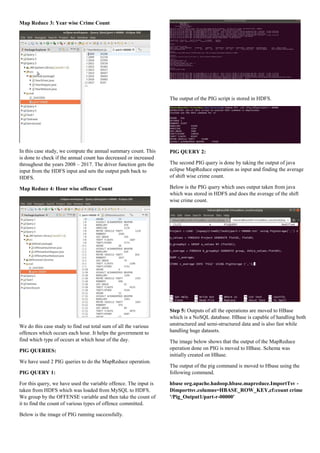
schema, which is then moved onto the HDFS using SQOOP for
further map reduce processing. The HDFS input is taken into
Java eclipse to perform the map reduce function and the output
is moved the NoSQL database – HBase. Further queries are
done on PIG. The output obtained from the map reduce
function and PIG query are visualized using R and Tableau for
better understanding.
Section 2 focuses on the related work done by various
researchers in the past. Section 3 contains information on the
selected technologies. Section 4 covers the methodologies used
in this project and section 5 and 6 covers the results obtained
and the future work.
II. RELATED WORK
In the recent past, various techniques are being using in
predicting where the next crime will take place, time – period
during which the crime will take place, etc. Machine learning
has been the most common way to do the tasks mentioned
above. In 2006, SVM was used to find Crime Hot-Spots, i.e., to
classify if a location is a crime hot spot or not. To do this, the
researcher has used spatial dataset and use one – class SVM for
predicting the hot-spot. In order to select the data, K-means
clustering algorithm was used and selected portion of the data
was labelled [1]. The researchers produced decent results by
using the one-class SVM. Another research was made using
similar kind of spatial databases and GIS. In this, various
machine algorithms such as Decision Tree, Support vector
machine (SVM), One Nearest Neighbour (INN), Naïve Bayes
and Neural network with 2-layer network were used [2]. The
overall performance of all the used methods were compared by
using them for over a 10-month period, during which, they
were compared based on the accuracy, precision, recall and F1.
The results produced show that the performance of a complex
algorithm is quite similar to the basic easy ones and INN
performs better. In another research conducted, the researchers
have used taxi flow data of the cities – Chicago and IL, and
have used linear regression and negative binomial regression.
The features used to do the regression were selected using
feature selected technique and the results obtained from the
regression models show that the features POI and taxi flow
reduces the prediction error by 17.6% [3]. In 2017, models
such as Z-CrimeTool, ID3 algorithm, hidden link detection,
Naïve Bayes used in a project to predict the crimes and the end
result shows that ID3 model performed better [4]. A similar
analysis was to find the crime hotspot in Taiwan and for this
analysis Big data containing the information on spatial data and
drug related criminal activity. To do this, data mining
classification methods such as random forest and Naïve Bayes
were used and visualizations with the crime hotspots were
plotted [5]. Naïve Bayes has been the most common method in
classifying / predicting the crime hotspot so far to predict the
Crime hotspot.

2. Rise in Big data has made it difficult to process the data, gain
insights and to use algorithms and hence to process big data,
Hadoop MapReduce environments are being preferred
currently. In this project, we analyse the big data of crime
using map reduce environments.
III. Chosen Technologies
MySQL: When it comes to an open source database
management system, MySQL is the 1st
choice as it can store
such big data and can perform well. Querying is also simple
and fast in MySQL and hence we have chosen the same to
store the initial dataset.
SQOOP: SQOOP is used as the mediator as it is a tool
designed to transfer big data fast and efficiently between
Hadoop ecosystem and relational databases. We have used
scoop to transfer the data since it can transfer data from the
relational database to Hadoop framework with the same
schema that was created in the relational database [6].
Java – Eclipse Environment: Eclipse is the most common
IDE used by programmers and it consists of basic work space
and plugins for customizing the environment. It consists of
Hadoop plugin and has by default mapper and reducer libraries
and uses Hadoop plugin to do the MapReduce function.
HBase: HBase is a NoSQL database which is used for storing
Large datasets. It is written in Java and is developed on top of
HDFS. HBase is column oriented database and it is similar to
google big table. Main advantage of HBase is that it is fault
tolerant, which means that data is not lost even if there is some
issue with the database. HBase is available open source and
hence HBase has been chosen to store the outputs from the
MapReduce functions.
PIG: PIG’s queries are simple and similar to MySQL queries
and PIG performs well with all kinds of dataset and does the
MapReduce functions well and is integrated with Hadoop
framework [7].
RStudio: RStudio is an open source IDE for R and is most
commonly used around the world as it is easy to programme in.
It uses various packages to do the analysis job. RStudio is the
choice for cleaning the dataset and for visualization.
IV. Methodology
Description of the Dataset:
The dataset that was used for this project is taken from
Kaggle - https://www.kaggle.com/vinchinzu/dc-metro-crime-
data. It contains the information on the crimes in Washington
DC and was last updated 1 year ago. The dataset contains the
information for the years 2008 – 2017 and contains the
following attributes (Only important attributes mentioned
below).
Attribute
name
Attribute
information
Selected/Reason
SHIFT Contains information
on shift of the day (Day,
Evening, Midnight)
Used to find shift
wise crime
OFFENSE Type of OFFENSE
done ( 10 Factors )
Used to find count of
each offence
year year of crime ( 2008 –
2017 )
Used to find year
wise crime
hour Hour during which
crime happened
( 0 – 23 )
Used to find hour
wise crime
date Date of the Crime not used
BLOCK Block where the crime
happened
not used
day Day in which the
crime happened
not used
minute Minute in which the
crime happened
not used
second Second in which the
crime happened
not used
month Month in which the
crime happened
not used
Data Processing:
(Flowchart done on Lucidchart -
https://www.lucidchart.com/documents/edit/3e8e4fe1-15fe-4f21-bc9c-
d3ee6f4ae404/0)
The Flowchart put up in the above image is the process that has
been followed in this project.
Step 1: The dataset used for this project is initially downloaded
by using ‘sudo wget https://www.kaggle.com/vinchinzu/dc-
metro-crime-data/downloads/dc-metro-crime-data.zip/5’ and is
stored on local machine initially.
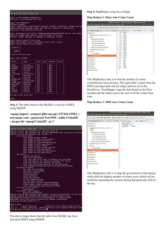
Step 2: The Dataset is then moved to MySQL after creating the
database – PDA, table CrimeDC and finally the proper Schema
of the table. The dataset is loaded into the created schema by
using –
load data local infile
'/home/kaushik/Downloads/CRIME DC.csv' into table
CrimeDC fields terminated by ',' lines terminated by
'n';
The image below shows the creation of schema, loading the
table into MySQL, table count and description of the table.

3. Step 3: The table stored in the MySQL is moved to HDFS
using SQOOP
‘sqoop import --connect jdbc:mysql://127.0.0.1/PDA --
username root --password Test1994 --table CrimeDC
--target-dir /sqoop/CrimeDC -m 1’
The above image shows that the table from MySQL has been
moved to HDFS using SQOOP.
Step 4: MapReduce using Java Eclipse
Map Reduce 1: Hour wise Crime Count
This MapReduce task is to find the number of crimes
committed per hour division. The input table is taken from the
HDFS and input path and the output path are set in the
HourDriver. HourMapper maps the data based on the Hour
variable and the reducer gives the sum of all the crimes hour
wise.
Map Reduce 2: Shift wise Crime Count
This MapReduce task is to help the government to find during
which shift the highest number of crimes occur which will be
useful for increasing the security during that particular shift of
the day.

4. Map Reduce 3: Year wise Crime Count
In this case study, we compute the annual summary count. This
is done to check if the annual count has decreased or increased
throughout the years 2008 – 2017. The driver function gets the
input from the HDFS input and sets the output path back to
HDFS.
Map Reduce 4: Hour wise offence Count
We do this case study to find out total sum of all the various
offences which occurs each hour. It helps the government to
find which type of occurs at which hour of the day.
PIG QUERIES:
We have used 2 PIG queries to do the MapReduce operation.
PIG QUERY 1:
For this query, we have used the variable offence. The input is
taken from HDFS which was loaded from MySQL to HDFS.
We group by the OFFENSE variable and then take the count of
it to find the count of various types of offence committed.
Below is the image of PIG running successfully.
The output of the PIG script is stored in HDFS.
PIG QUERY 2:
The second PIG query is done by taking the output of java
eclipse MapReduce operation as input and finding the average
of shift wise crime count.
Below is the PIG query which uses output taken from java
which was stored in HDFS and does the average of the shift
wise crime count.
Step 5: Outputs of all the operations are moved to HBase
which is a NoSQL database. HBase is capable of handling both
unstructured and semi-structured data and is also fast while
handling huge datasets.
The image below shows that the output of the MapReduce
operation done on PIG is moved to HBase. Schema was
initially created on HBase.
The output of the pig command is moved to Hbase using the
following command.
hbase org.apache.hadoop.hbase.mapreduce.ImportTsv -
Dimporttsv.columns=HBASE_ROW_KEY,cf:count crime
'/Pig_Output1/part-r-00000'

5. Step 6: The outputs are then taken out from HBase and moved
to local memory. The outputs are then visualized using ggplot2
in RStudio and Tableau.
V. Results and Visualization
This section covers the results of each of the operation carried
out using java eclipse and PIG. The outputs have been
visualized using RStudio and Tableau
MapReduce 1
The output of MapReduce operation 1 is visualized using line
graph on RStudio. The graph shows the hour-wise crime count
and it can be inferred that the crime rate peaks at the 15th
hour
of the day with crime count of 20,643 and hence, the
government can use this information to arrange better security
during this hour of the day.
MapReduce 2
The output of the 2nd
MapReduce task is to show the shift wise
crime count which is a consolidation of task 1, which covers
the hours of the day into different shifts. The choice of graph to
represent this output is bar graph, which is plotted in RStudio.
It can be inferred that, the highest number of crimes occur
during the evening time with the crime count value of 1,36,275
which is said to be the time during when drug sales peak,
which shows the correlation between the drug sales and crime
count. Second highest number of crimes occur during day time
with 1,23,014 crimes being record between the years 2008 –
2017.
MapReduce 3
Area graph has been chosen to represent the year wise increase
in crime rates and RStudio was the choice of visualization tool.
The graph shows that there is a dip in crime rate during the
years 2016 – 2017 but this is due to the fact that the data for
2017 was not updated with the info of crimes till the end of the
year. Apart from this, we can see that the crime rate has been
on constant increase from 2008-2016. The crime constantly
rising and it reaches the peak in the year 2014 with crime count
going up to 38,447.
MapReduce 4
Side by side Bar graph was used to show the Hour wise offence
count. The graph was done on Tableau. From the plot, we can
see that theft has been the most common type of crime and it
happens the most during the evening time which is the 15th
hour with the crime count reaching to the value of 9,554.

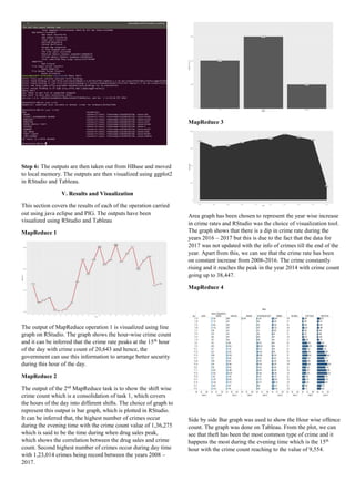
6. Pig 1
PIG Query is used to find the Crime Count by Offence. Tree
map is used to show the offence wise crime count which was
plotted using tableau. It can be inferred from the tree map that
theft has been the most common mode of offence followed by
robbery, motor vehicle theft, burglary and assault. Arson is the
least mode of offence committed.
Pig 2
Pig query is used to find the average of shift wise crime count.
Input for the query is taken from the MapReduce output. Bar
graph is used to represent the output visually and the results
show that on an average, more crimes occur during the evening
time.
VI. Conclusion and Future work
The motive of this project was to analyse the Crime Big
dataset to help the government set up better security to
decrease the crime rate in Washington DC. We have used the
technologies such as MySQL, HBase, Hadoop, Java, PIG,
RStudio and Tableau for analysing the data. The Big data was
analysed and visualized based on shift wise crime count, year
wise crime count, hour wise crime count and offense wise
crime count. The visualizations show that theft is the mostly
committed crime, most crime occur during the evening shift
and during the 15th
hour. From the results, we can also
understand that the crime rate has been constantly increasing
from the years 2008 to 2017. By using this information, the
government can act by increasing the security during the peak
hour to decrease the crime rate and to make the punishment
more severe for theft to decrease the theft count.
In the future, machine learning models can be done on pyspark
to predict the crime hotspot and when and how will a crime
happen in order to prevent the crime. Apart from that, apache
spark can be used instead of Hadoop framework as it is said to
be more efficient than Hadoop framework.
REFERENCES
[1] K. Kianmehr and R. Alhajj, "Crime Hot-Spots Prediction
Using Support Vector Machine," IEEE International
Conference on Computer Systems and Applications, 2006.,
Dubai, UAE, 2006, pp. 952-959.
doi: 10.1109/AICCSA.2006.205203
keywords: {Support vector machines;Data mining;Support
vector machine classification;Safety;Data analysis;Spatial
databases;Cities and towns;Computer science;Machine
learning;Geographic Information Systems},
URL: http://ieeexplore.ieee.org/stamp/stamp.jsp?tp=&arnumbe
r=1618468&isnumber=33913
[2] Yu, Jacky & Ward, Max & Morabito, Melissa & Ding,
Wei. (2011). Crime Forecasting Using Data Mining
Techniques. Proceedings - IEEE International Conference on
Data Mining, ICDM. 779-786. 10.1109/ICDMW.2011.56.
[3] Wang, Hongjian & Kifer, Daniel & Graif, Corina & Li,
Zhenhui. (2016). Crime Rate Inference with Big Data.
10.1145/2939672.2939736.
[4] C. Chauhan and S. Sehgal, "A review: Crime analysis using
data mining techniques and algorithms," 2017 International
Conference on Computing, Communication and Automation
(ICCCA), Greater Noida, 2017, pp. 21-25.
doi: 10.1109/CCAA.2017.8229823
keywords: {data analysis;data mining;police data
processing;data mining techniques;methodical
approach;trends;increasing origin;computerized systems;crime
data analysts;Law enforcement officers;unstructured
data;predictive policing means;analytical techniques;predictive
techniques;increased crime rate;criminals;crime
analysis;pattern identification;pattern analysis;crime
solving;advance technologies;Data mining;Tools;Algorithm
design and analysis;Classification
algorithms;Conferences;Forensics;Prediction algorithms;Data
Mining;crime analysis;Naive Bayes Classifiers;Predictive
approach},
URL: http://ieeexplore.ieee.org/stamp/stamp.jsp?tp=&arnumbe
r=8229823&isnumber=8229760
[5] Lin, Ying-Lung & Chen, Tenge-Yang & Yu, Liang-Chih.
(2017). Using Machine Learning to Assist Crime Prevention.
1029-1030. 10.1109/IIAI-AAI.2017.46.
[6] https://sqoop.apache.org/
[7] https://pig.apache.org/
[8] https://en.wikipedia.org/wiki/Crime_in_Washington,_
D.C.