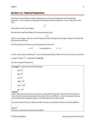
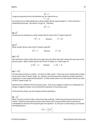
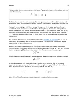
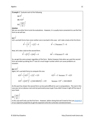
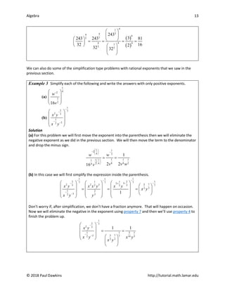
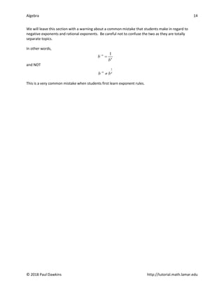
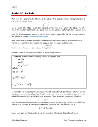
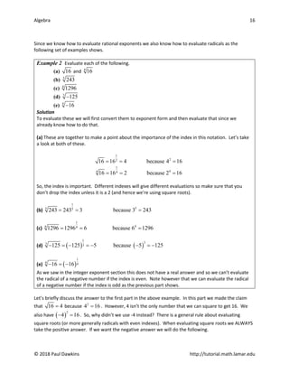
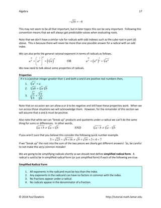
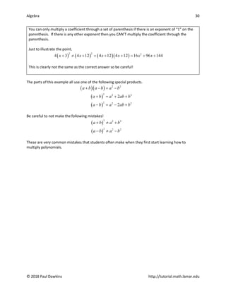
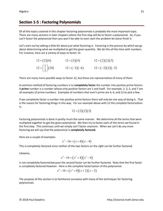
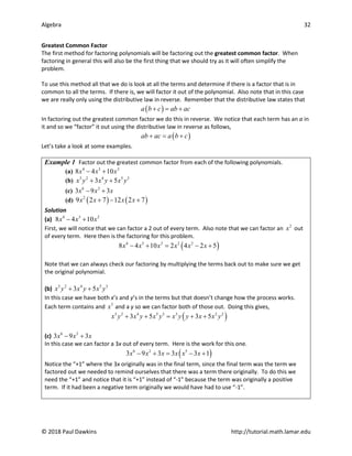
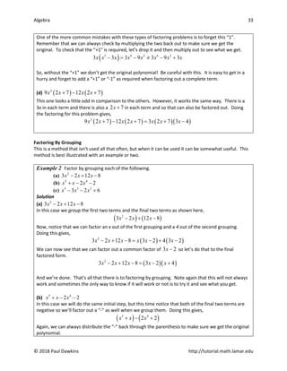
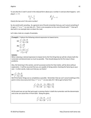
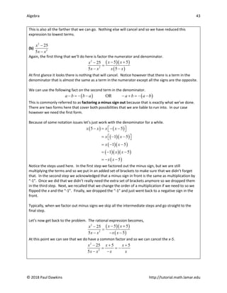
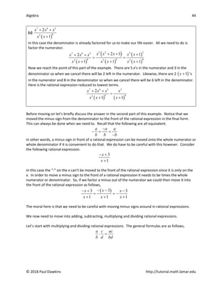
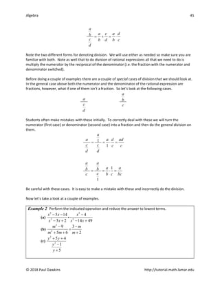
SlideShare a Scribd company logo
Preliminaries
Paul Dawkins
Algebra i
© 2018 Paul Dawkins http://tutorial.math.lamar.edu
Table of Contents
Preface ..................................................................................................................................................................ii
Chapter 1 : Preliminaries .......................................................................................................................................1
Section 1-1 : Integer Exponents ................................................................................................................................2
Section 1-2 : Rational Exponents...............................................................................................................................9
Section 1-3 : Radicals...............................................................................................................................................15
Section 1-4 : Polynomials ........................................................................................................................................25
Section 1-5 : Factoring Polynomials ........................................................................................................................31
Section 1-6 : Rational Expressions...........................................................................................................................41
Section 1-7 : Complex Numbers..............................................................................................................................52
Algebra ii
© 2018 Paul Dawkins http://tutorial.math.lamar.edu
Preface
Here are my online notes for my Algebra course that I teach here at Lamar University, although I
have to admit that it’s been years since I last taught this course. At this point in my career I
mostly teach Calculus and Differential Equations.
Despite the fact that these are my “class notes”, they should be accessible to anyone wanting to
learn Algebra or needing a refresher for Algebra. I’ve tried to make the notes as self contained
as possible and do not reference any book. However, they do assume that you’ve had some
exposure to the basics of algebra at some point prior to this. While there is some review of
exponents, factoring and graphing it is assumed that not a lot of review will be needed to
remind you how these topics work.
Here are a couple of warnings to my students who may be here to get a copy of what happened
on a day that you missed.
1. Because I wanted to make this a fairly complete set of notes for anyone wanting to learn
algebra I have included some material that I do not usually have time to cover in class
and because this changes from semester to semester it is not noted here. You will need
to find one of your fellow class mates to see if there is something in these notes that
wasn’t covered in class.
2. Because I want these notes to provide some more examples for you to read through, I
don’t always work the same problems in class as those given in the notes. Likewise,
even if I do work some of the problems in here I may work fewer problems in class than
are presented here.
3. Sometimes questions in class will lead down paths that are not covered here. I try to
anticipate as many of the questions as possible in writing these up, but the reality is that
I can’t anticipate all the questions. Sometimes a very good question gets asked in class
that leads to insights that I’ve not included here. You should always talk to someone
who was in class on the day you missed and compare these notes to their notes and see
what the differences are.
4. This is somewhat related to the previous three items but is important enough to merit
its own item. THESE NOTES ARE NOT A SUBSTITUTE FOR ATTENDING CLASS!! Using
these notes as a substitute for class is liable to get you in trouble. As already noted not
everything in these notes is covered in class and often material or insights not in these
notes is covered in class.
Algebra 1
© 2018 Paul Dawkins http://tutorial.math.lamar.edu
Chapter 1 : Preliminaries
The purpose of this chapter is to review several topics that will arise time and again throughout this
material. Many of the topics here are so important to an Algebra class that if you don’t have a good
working grasp of them you will find it very difficult to successfully complete the course. Also, it is
assumed that you’ve seen the topics in this chapter somewhere prior to this class and so this chapter
should be mostly a review for you. However, since most of these topics are so important to an Algebra
class we will make sure that you do understand them by doing a quick review of them here.
Exponents and polynomials are integral parts of any Algebra class. If you do not remember the basic
exponent rules and how to work with polynomials you will find it very difficult, if not impossible, to pass
an Algebra class. This is especially true with factoring polynomials. There are more than a few sections
in an Algebra course where the ability to factor is absolutely essential to being able to do the work in
those sections. In fact, in many of these sections factoring will be the first step taken.
It is important that you leave this chapter with a good understanding of this material! If you don’t
understand this material you will find it difficult to get through the remaining chapters. Here is a brief
listing of the material covered in this chapter.
Integer Exponents – In this section we will start looking at exponents. We will give the basic properties
of exponents and illustrate some of the common mistakes students make in working with exponents.
Examples in this section we will be restricted to integer exponents. Rational exponents will be discussed
in the next section.
Rational Exponents – In this section we will define what we mean by a rational exponent and extend the
properties from the previous section to rational exponents. We will also discuss how to evaluate
numbers raised to a rational exponent.
Radicals – In this section we will define radical notation and relate radicals to rational exponents. We
will also give the properties of radicals and some of the common mistakes students often make with
radicals. We will also define simplified radical form and show how to rationalize the denominator.
Polynomials – In this section we will introduce the basics of polynomials a topic that will appear
throughout this course. We will define the degree of a polynomial and discuss how to add, subtract and
multiply polynomials.
Factoring Polynomials – In this section we look at factoring polynomials a topic that will appear in pretty
much every chapter in this course and so is vital that you understand it. We will discuss factoring out
the greatest common factor, factoring by grouping, factoring quadratics and factoring polynomials with
degree greater than 2.
Rational Expressions – In this section we will define rational expressions. We will discuss how to reduce
a rational expression lowest terms and how to add, subtract, multiply and divide rational expressions.
Complex Numbers – In this section we give a very quick primer on complex numbers including standard
form, adding, subtracting, multiplying and dividing them.
Algebra 2
© 2018 Paul Dawkins http://tutorial.math.lamar.edu
Section 1-1 : Integer Exponents
We will start off this chapter by looking at integer exponents. In fact, we will initially assume that the
exponents are positive as well. We will look at zero and negative exponents in a bit.
Let’s first recall the definition of exponentiation with positive integer exponents. If a is any number and
n is a positive integer then,
times
n
n
a a a a a
= ⋅ ⋅ ⋅ ⋅


So, for example,
5
3 3 3 3 3 3 243
= ⋅ ⋅ ⋅ ⋅ =
We should also use this opportunity to remind ourselves about parenthesis and conventions that we
have in regard to exponentiation and parenthesis. This will be particularly important when dealing with
negative numbers. Consider the following two cases.
( )
4 4
2 and 2
− −
These will have different values once we evaluate them. When performing exponentiation remember
that it is only the quantity that is immediately to the left of the exponent that gets the power.
In the first case there is a parenthesis immediately to the left so that means that everything in the
parenthesis gets the power. So, in this case we get,
( ) ( )( )( )( )
4
2 2 2 2 2 16
− =− − − − =
In the second case however, the 2 is immediately to the left of the exponent and so it is only the 2 that
gets the power. The minus sign will stay out in front and will NOT get the power. In this case we have
the following,
( ) ( ) ( )
4 4
2 2 2 2 2 2 16 16
− =
− =
− ⋅ ⋅ ⋅ =
− =
−
We put in some extra parenthesis to help illustrate this case. In general, they aren’t included and we
would write instead,
4
2 2 2 2 2 16
− =
− ⋅ ⋅ ⋅ =
−
The point of this discussion is to make sure that you pay attention to parenthesis. They are important
and ignoring parenthesis or putting in a set of parenthesis where they don’t belong can completely
change the answer to a problem. Be careful. Also, this warning about parenthesis is not just intended
for exponents. We will need to be careful with parenthesis throughout this course.
Now, let’s take care of zero exponents and negative integer exponents. In the case of zero exponents we
have,
0
1 provided 0
a a
= ≠
Notice that it is required that a not be zero. This is important since 0
0 is not defined. Here is a quick
example of this property.
( )
0
1268 1
− =
Algebra 3
© 2018 Paul Dawkins http://tutorial.math.lamar.edu
We have the following definition for negative exponents. If a is any non-zero number and n is a positive
integer (yes, positive) then,
1
n
n
a
a
−
=
Can you see why we required that a not be zero? Remember that division by zero is not defined and if
we had allowed a to be zero we would have gotten division by zero. Here are a couple of quick
examples for this definition,
( )
( )
3
2
3
2
1 1 1 1 1
5 4
5 25 64 64
4
−
−
== − = = =
−
−
−
Here are some of the main properties of integer exponents. Accompanying each property will be a
quick example to illustrate its use. We will be looking at more complicated examples after the
properties.
Properties
1. n m n m
a a a +
= Example : 9 4 9 4 5
a a a a
− − + −
= =
2. ( )
m
n nm
a a
= Example : ( ) ( )( )
3 7 3
7 21
a a a
= =
3. , 0
1
n m
n
m
m n
a
a
a
a
a
−
−


= ≠



Example :
4
4 11 7
11
4
7
11 11 4 7
1 1
a
a a
a
a
a
a a a
− −
−
−
= =
= = =
4. ( )
n n n
ab a b
= Example : ( )
4 4 4
ab a b
− − −
=
5. , 0
n n
n
a a
b
b b
 
= ≠
 
 
Example :
8 8
8
a a
b b
 
=
 
 
6.
n n n
n
a b b
b a a
−
   
= =
   
   
Example :
10 10 10
10
a b b
b a a
−
   
= =
   
   
7. ( )
( )
1
n
n
ab
ab
−
= Example : ( )
( )
20
20
1
ab
ab
−
=
8.
1 n
n
a
a−
= Example : 2
2
1
a
a−
=
Algebra 4
© 2018 Paul Dawkins http://tutorial.math.lamar.edu
9.
n m
m n
a b
b a
−
−
= Example :
6 17
17 6
a b
b a
−
−
=
10. ( )
k
n m nk mk
a b a b
= Example : ( ) ( )( ) ( )( )
3 4 3 9 3
4 9 12 27
a b a b a b
−
− −
= =
11.
k
n nk
m mk
a a
b b
 
=
 
 
Example :
( )( )
( )( )
2 6 2
6 12
5 10
5 2
a a a
b b
b
 
= =
 
 
Notice that there are two possible forms for the third property. Which form you use is usually
dependent upon the form you want the answer to be in.
Note as well that many of these properties were given with only two terms/factors but they can be
extended out to as many terms/factors as we need. For example, property 4 can be extended as
follows.
( )
n n n n n
abcd a b c d
=
We only used four factors here, but hopefully you get the point. Property 4 (and most of the other
properties) can be extended out to meet the number of factors that we have in a given problem.
There are several common mistakes that students make with these properties the first time they see
them. Let’s take a look at a couple of them.
Consider the following case.
2
2 2
2
2
1
Correct :
1
Incorrect :
a
ab a
b b
ab
ab
−
−
= =
≠
In this case only the b gets the exponent since it is immediately off to the left of the exponent and so
only this term moves to the denominator. Do NOT carry the a down to the denominator with the b.
Contrast this with the following case.
( )
( )
2
2
1
ab
ab
−
=
In this case the exponent is on the set of parenthesis and so we can just use property 7 on it and so both
the a and the b move down to the denominator. Again, note the importance of parenthesis and how
they can change an answer!
Here is another common mistake.
5
5 5
5
5
1 1 1 1
Correct :
3 3 3
1
Incorrect : 3
3
a
a a
a
a
− −
−
= =
≠
Algebra 5
© 2018 Paul Dawkins http://tutorial.math.lamar.edu
In this case the exponent is only on the a and so to use property 8 on this we would have to break up
the fraction as shown and then use property 8 only on the second term. To bring the 3 up with the a we
would have needed the following.
( )
( )
5
5
1
3
3
a
a
−
=
Once again, notice this common mistake comes down to being careful with parenthesis. This will be a
constant refrain throughout these notes. We must always be careful with parenthesis. Misusing them
can lead to incorrect answers.
Let’s take a look at some more complicated examples now.
Example 1 Simplify each of the following and write the answers with only positive exponents.
(a) ( )
3
4 5
4x y
−
(b) ( ) ( )
2 5
2 4 3
10z y z y
−
−
−
(c)
2
4 3
7
n m
m n
−
− −
(d)
( )
1 4
2
5 9
5
3
x y
y x
− −
−
(e)
6
5
2 1
z
z x
−
− −
 
 
 
(f)
2
3 8
5
24
6
a b
a b
−
−
−
 
 
 
Solution
Note that when we say “simplify” in the problem statement we mean that we will need to use all the
properties that we can to get the answer into the required form. Also, a “simplified” answer will have
as few terms as possible and each term should have no more than a single exponent on it.
There are many different paths that we can take to get to the final answer for each of these. In the
end the answer will be the same regardless of the path that you used to get the answer. All that this
means for you is that as long as you used the properties you can take the path that you find the
easiest. The path that others find to be the easiest may not be the path that you find to be the
easiest. That is okay.
Also, we won’t put quite as much detail in using some of these properties as we did in the examples
given with each property. For instance, we won’t show the actual multiplications anymore, we will
just give the result of the multiplication.
Algebra 6
© 2018 Paul Dawkins http://tutorial.math.lamar.edu
(a) ( )
3
4 5
4x y
−
For this one we will use property 10 first.
( )
3
4 5 3 12 15
4 4
x y x y
− −
=
Don’t forget to put the exponent on the constant in this problem. That is one of the more common
mistakes that students make with these simplification problems.
At this point we need to evaluate the first term and eliminate the negative exponent on the second
term. The evaluation of the first term isn’t too bad and all we need to do to eliminate the negative
exponent on the second term is use the definition we gave for negative exponents.
( )
15
3
4 5 15
12 12
1 64
4 64
y
x y y
x x
−  
= =
 
 
We further simplified our answer by combining everything up into a single fraction. This should
always be done.
The middle step in this part is usually skipped. All the definition of negative exponents tells us to do is
move the term to the denominator and drop the minus sign in the exponent. So, from this point on,
that is what we will do without writing in the middle step.
(b) ( ) ( )
2 5
2 4 3
10z y z y
−
−
−
In this case we will first use property 10 on both terms and then we will combine the terms using
property 1. Finally, we will eliminate the negative exponents using the definition of negative
exponents.
( ) ( ) ( )
2 5 2
2 4 3 4 8 15 5 11 13
11 13
100
10 10 100
z y z y z y z y z y
z y
−
− − − − − −
− =
− =
=
There are a couple of things to be careful with in this problem. First, when using the property 10 on
the first term, make sure that you square the “-10” and not just the 10 (i.e. don’t forget the minus
sign…). Second, in the final step, the 100 stays in the numerator since there is no negative exponent
on it. The exponent of “-11” is only on the z and so only the z moves to the denominator.
(c)
2
4 3
7
n m
m n
−
− −
This one isn’t too bad. We will use the definition of negative exponents to move all terms with
negative exponents in them to the denominator. Also, property 8 simply says that if there is a term
with a negative exponent in the denominator then we will just move it to the numerator and drop the
minus sign.
So, let’s take care of the negative exponents first.
2 4 3
4 3 2
7 7
n m m n m
m n n
−
− −
=
Algebra 7
© 2018 Paul Dawkins http://tutorial.math.lamar.edu
Now simplify. We will use property 1 to combine the m’s in the numerator. We will use property 3 to
combine the n’s and since we are looking for positive exponents we will use the first form of this
property since that will put a positive exponent up in the numerator.
2 5
4 3
7 7
n m m n
m n
−
− −
=
Again, the 7 will stay in the denominator since there isn’t a negative exponent on it. It will NOT move
up to the numerator with the m. Do not get excited if all the terms move up to the numerator or if all
the terms move down to the denominator. That will happen on occasion.
(d)
( )
1 4
2
5 9
5
3
x y
y x
− −
−
This example is similar to the previous one except there is a little more going on with this one. The
first step will be to again, get rid of the negative exponents as we did in the previous example. Any
terms in the numerator with negative exponents will get moved to the denominator and we’ll drop
the minus sign in the exponent. Likewise, any terms in the denominator with negative exponents will
move to the numerator and we’ll drop the minus sign in the exponent. Notice this time, unlike the
previous part, there is a term with a set of parenthesis in the denominator. Because of the
parenthesis that whole term, including the 3, will move to the numerator.
Here is the work for this part.
( )
( ) ( )
2
5 10
1 4 6
2 4 9 4 9 10
5 9
5 3 5 9
5 45
3
y y
x y y
xy x xy x x
y x
− −
−
= = =
(e)
6
5
2 1
z
z x
−
− −
 
 
 
There are several first steps that we can take with this one. The first step that we’re pretty much
always going to take with these kinds of problems is to first simplify the fraction inside the
parenthesis as much as possible. After we do that we will use property 5 to deal with the exponent
that is on the parenthesis.
6 6 6
5 2 1 6
2 1 5 3 18
z z x x x
z x z z z
−
− −
     
= = =
     
 
   
In this case we used the second form of property 3 to simplify the z’s since this put a positive
exponent in the denominator. Also note that we almost never write an exponent of “1”. When we
have exponents of 1 we will drop them.
(f)
2
3 8
5
24
6
a b
a b
−
−
−
 
 
 
This one is very similar to the previous part. The main difference is negative on the outer exponent.
We will deal with that once we’ve simplified the fraction inside the parenthesis.
Algebra 8
© 2018 Paul Dawkins http://tutorial.math.lamar.edu
2 2 2
3 8 3 5 8
5 8 9
24 4 4
6
a b a a a
a b b b b
− − −
−
−
     
= =
     
     
Now at this point we can use property 6 to deal with the exponent on the parenthesis. Doing this
gives us,
2 2
3 8 9 18
5 8 16
24
6 4 16
a b b b
a b a a
−
−
−
   
= =
   
   
Before leaving this section we need to talk briefly about the requirement of positive only exponents in
the above set of examples. This was done only so there would be a consistent final answer. In many
cases negative exponents are okay and in some cases they are required. In fact, if you are on a track
that will take you into calculus there are a fair number of problems in a calculus class in which negative
exponents are the preferred, if not required, form.
Algebra 9
© 2018 Paul Dawkins http://tutorial.math.lamar.edu
Section 1-2 : Rational Exponents
Now that we have looked at integer exponents we need to start looking at more complicated
exponents. In this section we are going to be looking at rational exponents. That is exponents in the
form
m
n
b
where both m and n are integers.
We will start simple by looking at the following special case,
1
n
b
where n is an integer. Once we have this figured out the more general case given above will actually be
pretty easy to deal with.
Let’s first define just what we mean by exponents of this form.
1
is equivalent to n
n
a b a b
= =
In other words, when evaluating
1
n
b we are really asking what number (in this case a) did we raise to the
n to get b. Often
1
n
b is called the nth
root of b.
Let’s do a couple of evaluations.
Example 1 Evaluate each of the following.
(a)
1
2
25
(b)
1
5
32
(c)
1
4
81
(d) ( )
1
3
8
−
(e) ( )
1
4
16
−
(f)
1
4
16
−
Solution
When doing these evaluations, we will not actually do them directly. When first confronted with
these kinds of evaluations doing them directly is often very difficult. In order to evaluate these we
will remember the equivalence given in the definition and use that instead.
We will work the first one in detail and then not put as much detail into the rest of the problems.
(a)
1
2
25
So, here is what we are asking in this problem.
Algebra 10
© 2018 Paul Dawkins http://tutorial.math.lamar.edu
1
2
25 ?
=
Using the equivalence from the definition we can rewrite this as,
2
? 25
=
So, all that we are really asking here is what number did we square to get 25. In this case that is
(hopefully) easy to get. We square 5 to get 25. Therefore,
1
2
25 5
=
(b)
1
5
32
So what we are asking here is what number did we raise to the 5th
power to get 32?
1
5
5
32 2 because 2 32
= =
(c)
1
4
81
What number did we raise to the 4th
power to get 81?
1
4
4
81 3 because 3 81
= =
(d) ( )
1
3
8
−
We need to be a little careful with minus signs here, but other than that it works the same way as the
previous parts. What number did we raise to the 3rd
power (i.e. cube) to get -8?
( ) ( )
1
3
3
8 2 because 2 8
− =
− − =
−
(e) ( )
1
4
16
−
This part does not have an answer. It is here to make a point. In this case we are asking what number
do we raise to the 4th
power to get -16. However, we also know that raising any number (positive or
negative) to an even power will be positive. In other words, there is no real number that we can raise
to the 4th
power to get -16.
Note that this is different from the previous part. If we raise a negative number to an odd power we
will get a negative number so we could do the evaluation in the previous part.
As this part has shown, we can’t always do these evaluations.
(f)
1
4
16
−
Again, this part is here to make a point more than anything. Unlike the previous part this one has an
answer. Recall from the previous section that if there aren’t any parentheses then only the part
immediately to the left of the exponent gets the exponent. So, this part is really asking us to evaluate
the following term.
1 1
4 4
16 16
 
− =
− 
 
Algebra 11
© 2018 Paul Dawkins http://tutorial.math.lamar.edu
So, we need to determine what number raised to the 4th
power will give us 16. This is 2 and so in this
case the answer is,
( )
1 1
4 4
16 16 2 2
 
− =
− =
− =
−
 
 
As the last two parts of the previous example has once again shown, we really need to be careful with
parenthesis. In this case parenthesis makes the difference between being able to get an answer or not.
Also, don’t be worried if you didn’t know some of these powers off the top of your head. They are
usually fairly simple to determine if you don’t know them right away. For instance, in the part b we
needed to determine what number raised to the 5 will give 32. If you can’t see the power right off the
top of your head simply start taking powers until you find the correct one. In other words compute 5
2 ,
5
3 , 5
4 until you reach the correct value. Of course, in this case we wouldn’t need to go past the first
computation.
The next thing that we should acknowledge is that all of the properties for exponents that we gave in
the previous section are still valid for all rational exponents. This includes the more general rational
exponent that we haven’t looked at yet.
Now that we know that the properties are still valid we can see how to deal with the more general
rational exponent. There are in fact two different ways of dealing with them as we’ll see. Both methods
involve using property 2 from the previous section. For reference purposes this property is,
( )
m
n nm
a a
=
So, let’s see how to deal with a general rational exponent. We will first rewrite the exponent as follows.
( )
1
m m
n
n
b b
 
 
 
=
In other words, we can think of the exponent as a product of two numbers. Now we will use the
exponent property shown above. However, we will be using it in the opposite direction than what we
did in the previous section. Also, there are two ways to do it. Here they are,
( )
1 1
OR
m
m m
m
n n n n
b b b b
 
= =
 
 
Using either of these forms we can now evaluate some more complicated expressions
Algebra 12
© 2018 Paul Dawkins http://tutorial.math.lamar.edu
Example 2 Evaluate each of the following.
(a)
2
3
8
(b)
3
4
625
(c)
4
5
243
32
 
 
 
Solution
We can use either form to do the evaluations. However, it is usually more convenient to use the first
form as we will see.
(a)
2
3
8
Let’s use both forms here since neither one is too bad in this case. Let’s take a look at the first form.
( )
2
2 1 1
2 3
3 3 3
8 8 2 4 8 2 because 2 8
 
= = = = =
 
 
Now, let’s take a look at the second form.
( ) ( )
2 1
1 1
2 3
3 3
3 3
8 8 64 4 64 4 because 4 64
= = = = =
So, we get the same answer regardless of the form. Notice however that when we used the second
form we ended up taking the 3rd
root of a much larger number which can cause problems on
occasion.
(b)
3
4
625
Again, let’s use both forms to compute this one.
( )
3
3 1 1
3 4
4 4 4
625 625 5 125 625 5 because 5 625
 
= = = = =
 
 
( ) ( )
3 1 1
3 4
4 4 4
625 625 244140625 125 because 125 244140625
= = = =
As this part has shown the second form can be quite difficult to use in computations. The root in this
case was not an obvious root and not particularly easy to get if you didn’t know it right off the top of
your head.
(c)
4
5
243
32
 
 
 
In this case we’ll only use the first form. However, before doing that we’ll need to first use property 5
of our exponent properties to get the exponent onto the numerator and denominator.
Algebra 13
© 2018 Paul Dawkins http://tutorial.math.lamar.edu
( )
( )
4
1
5
4
4 4
5
5
4 4 4
1
5 5
243
3
243 243 81
32 16
2
32 32
 
 
   
= = = =
 
   
 
 
We can also do some of the simplification type problems with rational exponents that we saw in the
previous section.
Example 3 Simplify each of the following and write the answers with only positive exponents.
(a)
1
4
2
1
2
16
w
v
−
 
 
 
 
(b)
1
2 7
2 3
1
3
2
x y
x y
−
−
−
−
 
 
 
 
 
Solution
(a) For this problem we will first move the exponent into the parenthesis then we will eliminate the
negative exponent as we did in the previous section. We will then move the term to the denominator
and drop the minus sign.
1 1
2
4 2
1 1 1
1 1
1
8 8 2
2 4
4
1
2 2
16
w w
v v w
v
 
− −
 
 
 
 
 
= =
(b) In this case we will first simplify the expression inside the parenthesis.
1 1
1
1
2 2
1 1
7 7
7 3
2 7
5
2 2 3 7
3 3
2 2
3
2
1 2
3
2 3
1
x y x x y x y
x y
x y y
− −
−
−
− −
+
−
−
   
 
 
   
 
= = =  
   
 
   
   
 
   
Don’t worry if, after simplification, we don’t have a fraction anymore. That will happen on occasion.
Now we will eliminate the negative in the exponent using property 7 and then we’ll use property 4 to
finish the problem up.
1
2 7
2 3
1 1 1
5
7
5
3
2 7 3
14
3
2
1 1
x y
x y x y
x y
−
−
−
−
 
 
= =
 
   
 
 
 
Algebra 14
© 2018 Paul Dawkins http://tutorial.math.lamar.edu
We will leave this section with a warning about a common mistake that students make in regard to
negative exponents and rational exponents. Be careful not to confuse the two as they are totally
separate topics.
In other words,
1
n
n
b
b
−
=
and NOT
1
n n
b b
−
≠
This is a very common mistake when students first learn exponent rules.
Algebra 15
© 2018 Paul Dawkins http://tutorial.math.lamar.edu
Section 1-3 : Radicals
We’ll open this section with the definition of the radical. If n is a positive integer that is greater than 1
and a is a real number then,
1
n n
a a
=
where n is called the index, a is called the radicand, and the symbol is called the radical. The left
side of this equation is often called the radical form and the right side is often called the exponent form.
From this definition we can see that a radical is simply another notation for the first rational exponent
that we looked at in the rational exponents section.
Note as well that the index is required in these to make sure that we correctly evaluate the radical.
There is one exception to this rule and that is square root. For square roots we have,
2
a a
=
In other words, for square roots we typically drop the index.
Let’s do a couple of examples to familiarize us with this new notation.
Example 1 Write each of the following radicals in exponent form.
(a) 4
16
(b) 10
8x
(c) 2 2
x y
+
Solution
(a)
1
4 4
16 16
=
(b) ( )
1
10 10
8 8
x x
=
(c) ( )
1
2 2 2 2 2
x y x y
+ = +
As seen in the last two parts of this example we need to be careful with parenthesis. When we convert
to exponent form and the radicand consists of more than one term then we need to enclose the whole
radicand in parenthesis as we did with these two parts. To see why this is consider the following,
1
10
8x
From our discussion of exponents in the previous sections we know that only the term immediately to
the left of the exponent actually gets the exponent. Therefore, the radical form of this is,
1
10 10
10
8 8 8
x x x
= ≠
So, we once again see that parenthesis are very important in this class. Be careful with them.
Algebra 16
© 2018 Paul Dawkins http://tutorial.math.lamar.edu
Since we know how to evaluate rational exponents we also know how to evaluate radicals as the
following set of examples shows.
Example 2 Evaluate each of the following.
(a) 16 and 4
16
(b) 5
243
(c) 4
1296
(d) 3
125
−
(e) 4
16
−
Solution
To evaluate these we will first convert them to exponent form and then evaluate that since we
already know how to do that.
(a) These are together to make a point about the importance of the index in this notation. Let’s take
a look at both of these.
1
2
2
16 16 4 because 4 16
= = =
1
4
4 4
16 16 2 because 2 16
= = =
So, the index is important. Different indexes will give different evaluations so make sure that you
don’t drop the index unless it is a 2 (and hence we’re using square roots).
(b)
1
5
5 5
243 243 3 because 3 243
= = =
(c)
1
4
4 4
1296 1296 6 because 6 1296
= = =
(d) ( ) ( )
1
3
3 3
125 125 5 because 5 125
− =
− =
− − =
−
(e) ( )
1
4 4
16 16
− =−
As we saw in the integer exponent section this does not have a real answer and so we can’t evaluate
the radical of a negative number if the index is even. Note however that we can evaluate the radical
of a negative number if the index is odd as the previous part shows.
Let’s briefly discuss the answer to the first part in the above example. In this part we made the claim
that 16 4
= because 2
4 16
= . However, 4 isn’t the only number that we can square to get 16. We
also have ( )
2
4 16
− =
. So, why didn’t we use -4 instead? There is a general rule about evaluating
square roots (or more generally radicals with even indexes). When evaluating square roots we ALWAYS
take the positive answer. If we want the negative answer we will do the following.
Algebra 17
© 2018 Paul Dawkins http://tutorial.math.lamar.edu
16 4
− =
−
This may not seem to be all that important, but in later topics this can be very important. Following this
convention means that we will always get predictable values when evaluating roots.
Note that we don’t have a similar rule for radicals with odd indexes such as the cube root in part (d)
above. This is because there will never be more than one possible answer for a radical with an odd
index.
We can also write the general rational exponent in terms of radicals as follows.
( ) ( )
1 1
OR
m
m m
m
n
m m
n
n n n n
a a a a a a
 
= = = =
 
 
We now need to talk about some properties of radicals.
Properties
If n is a positive integer greater than 1 and both a and b are positive real numbers then,
1.
n n
a a
=
2. n n n
ab a b
=
3.
n
n
n
a a
b b
=
Note that on occasion we can allow a or b to be negative and still have these properties work. When we
run across those situations we will acknowledge them. However, for the remainder of this section we
will assume that a and b must be positive.
Also note that while we can “break up” products and quotients under a radical we can’t do the same
thing for sums or differences. In other words,
AND
n n n n n n
a b a b a b a b
+ ≠ + − ≠ −
If you aren’t sure that you believe this consider the following quick number example.
5 25 9 16 9 16 3 4 7
= = + ≠ + = + =
If we “break up” the root into the sum of the two pieces we clearly get different answers! So, be careful
to not make this very common mistake!
We are going to be simplifying radicals shortly so we should next define simplified radical form. A
radical is said to be in simplified radical form (or just simplified form) if each of the following are true.
Simplified Radical Form
1. All exponents in the radicand must be less than the index.
2. Any exponents in the radicand can have no factors in common with the index.
3. No fractions appear under a radical.
4. No radicals appear in the denominator of a fraction.
Algebra 18
© 2018 Paul Dawkins http://tutorial.math.lamar.edu
In our first set of simplification examples we will only look at the first two. We will need to do a little
more work before we can deal with the last two.
Example 3 Simplify each of the following. Assume that x, y, and z are positive.
(a) 7
y
(b)
9 6
x
(c) 6 11
18x y
(d) 9 5 12
4
32x y z
(e) 12 4 24
5
x y z
(f) 3 3
2 2
9 6
x x
Solution
(a) 7
y
In this case the exponent (7) is larger than the index (2) and so the first rule for simplification is
violated. To fix this we will use the first and second properties of radicals above. So, let’s note that
we can write the radicand as follows.
( )
2
7 6 3
y y y y y
= =
So, we’ve got the radicand written as a perfect square times a term whose exponent is smaller than
the index. The radical then becomes,
( )
2
7 3
y y y
=
Now use the second property of radicals to break up the radical and then use the first property of
radicals on the first term.
( )
2
7 3 3
y y y y y
= =
This now satisfies the rules for simplification and so we are done.
Before moving on let’s briefly discuss how we figured out how to break up the exponent as we did.
To do this we noted that the index was 2. We then determined the largest multiple of 2 that is less
than 7, the exponent on the radicand. This is 6. Next, we noticed that 7=6+1.
Finally, remembering several rules of exponents we can rewrite the radicand as,
( )( )
( )
2
3 2
7 6 3
y y y y y y y
= = =
In the remaining examples we will typically jump straight to the final form of this and leave the details
to you to check.
Algebra 19
© 2018 Paul Dawkins http://tutorial.math.lamar.edu
(b) 9 6
x
This radical violates the second simplification rule since both the index and the exponent have a
common factor of 3. To fix this all we need to do is convert the radical to exponent form do some
simplification and then convert back to radical form.
( ) ( )
6 2
1 1
9 3
6 6 2 2
9 3
9 3
x x x x x x
= = = = =
(c) 6 11
18x y
Now that we’ve got a couple of basic problems out of the way let’s work some harder ones.
Although, with that said, this one is really nothing more than an extension of the first example.
There is more than one term here but everything works in exactly the same fashion. We will break
the radicand up into perfect squares times terms whose exponents are less than 2 (i.e. 1).
( ) ( ) ( ) ( )
2 2
6 11 6 10 3 5
18 9 2 9 2
x y x y y x y y
= =
Don’t forget to look for perfect squares in the number as well.
Now, go back to the radical and then use the second and first property of radicals as we did in the first
example.
( ) ( ) ( ) ( ) ( )
2 2 2 2
6 11 3 5 3 5 3 5
18 9 2 9 2 3 2
x y x y y x y y x y y
= = =
Note that we used the fact that the second property can be expanded out to as many terms as we
have in the product under the radical. Also, don’t get excited that there are no x’s under the radical in
the final answer. This will happen on occasion.
(d) 9 5 12
4
32x y z
This one is similar to the previous part except the index is now a 4. So, instead of get perfect squares
we want powers of 4. This time we will combine the work in the previous part into one step.
( ) ( ) ( )
4 4
9 5 12 8 4 12 2 4 3 2 3
4
4 4
4 4 4 4
4
32 16 2 16 2 2 2
x y z x y z xy x y z xy x y z xy
= = =
(e) 12 4 24
5
x y z
Again this one is similar to the previous two parts.
( ) ( ) ( )
5 5
12 4 24 10 20 2 4 4 2 4 2 4 4 2 4 2 4 4
5 5 5
5 5
5
x y z x z x y z x z x y z x z x y z
= = =
In this case don’t get excited about the fact that all the y’s stayed under the radical. That will happen
on occasion.
(f) 3 3
2 2
9 6
x x
This last part seems a little tricky. Individually both of the radicals are in simplified form. However,
there is often an unspoken rule for simplification. The unspoken rule is that we should have as few
radicals in the problem as possible. In this case that means that we can use the second property of
Algebra 20
© 2018 Paul Dawkins http://tutorial.math.lamar.edu
radicals to combine the two radicals into one radical and then we’ll see if there is any simplification
that needs to be done.
( )( )
3 3 3
2 2 2 2 4
3
9 6 9 6 54
x x x x x
= =
Now that it’s in this form we can do some simplification.
( )
3 3 3
2 2 3 3 3 3
3
9 6 27 2 27 2 3 2
x x x x x x x x
= = =
Before moving into a set of examples illustrating the last two simplification rules we need to talk briefly
about adding/subtracting/multiplying radicals. Performing these operations with radicals is much the
same as performing these operations with polynomials. If you don’t remember how to
add/subtract/multiply polynomials we will give a quick reminder here and then give a more in depth set
of examples the next section.
Recall that to add/subtract terms with x in them all we need to do is add/subtract the coefficients of the
x. For example,
( ) ( )
4 9 4 9 13 3 11 3 11 8
x x x x x x x x
+ =+ = − =− =
−
Adding/subtracting radicals works in exactly the same manner. For instance,
( ) ( )
10 10 10 10
4 9 4 9 13 3 5 11 5 3 11 5 8 5
x x x x
+ =
+ = − =
− =
−
We’ve already seen some multiplication of radicals in the last part of the previous example. If we are
looking at the product of two radicals with the same index then all we need to do is use the second
property of radicals to combine them then simplify. What we need to look at now are problems like the
following set of examples.
Example 4 Multiply each of the following. Assume that x is positive.
(a) ( )( )
2 5
x x
+ −
(b) ( )( )
3 2 5
x y x y
− −
(c) ( )( )
5 2 5 2
x x
+ −
Solution
In all of these problems all we need to do is recall how to FOIL binomials. Recall,
( )( ) ( ) ( ) ( ) ( ) 2 2
3 5 2 3 3 2 5 5 2 3 6 5 10 3 10
x x x x x x x x x x x
− + = + − − = + − − = + −
With radicals we multiply in exactly the same manner. The main difference is that on occasion we’ll
need to do some simplification after doing the multiplication
Algebra 21
© 2018 Paul Dawkins http://tutorial.math.lamar.edu
(a) ( )( )
2 5
x x
+ −
( )( ) ( )
2
2 5 5 2 10
3 10
3 10
x x x x x x
x x
x x
+ −
= − + −
= − −
=
− −
As noted above we did need to do a little simplification on the first term after doing the
multiplication.
(b) ( )( )
3 2 5
x y x y
− −
Don’t get excited about the fact that there are two variables here. It works the same way!
( )( ) 2 2
3 2 5 6 15 2 5
6 15 2 5
6 17 5
x y x y x x y x y y
x xy xy y
x xy y
− − = − − +
= − − +
=− +
Again, notice that we combined up the terms with two radicals in them.
(c) ( )( )
5 2 5 2
x x
+ −
Not much to do with this one.
( )( ) 2
5 2 5 2 25 10 10 4 25 4
x x x x x x
+ − = − + − = −
Notice that, in this case, the answer has no radicals. That will happen on occasion so don’t get excited
about it when it happens.
The last part of the previous example really used the fact that
( )( ) 2 2
a b a b a b
+ − = −
If you don’t recall this formula we will look at it in a little more detail in the next section.
Okay, we are now ready to take a look at some simplification examples illustrating the final two rules.
Note as well that the fourth rule says that we shouldn’t have any radicals in the denominator. To get rid
of them we will use some of the multiplication ideas that we looked at above and the process of getting
rid of the radicals in the denominator is called rationalizing the denominator. In fact, that is really what
this next set of examples is about. They are really more examples of rationalizing the denominator
rather than simplification examples.
Algebra 22
© 2018 Paul Dawkins http://tutorial.math.lamar.edu
Example 5 Rationalize the denominator for each of the following. Assume that x is positive.
(a)
4
x
(b) 5
3
2
x
(c)
1
3 x
−
(d)
5
4 3
x +
Solution
There are really two different types of problems that we’ll be seeing here. The first two parts
illustrate the first type of problem and the final two parts illustrate the second type of problem. Both
types are worked differently.
(a)
4
x
In this case we are going to make use of the fact that n n
a a
= . We need to determine what to
multiply the denominator by so that this will show up in the denominator. Once we figure this out we
will multiply the numerator and denominator by this term.
Here is the work for this part.
2
4 4 4 4
x x x
x
x x x x
= = =
Remember that if we multiply the denominator by a term we must also multiply the numerator by the
same term. In this way we are really multiplying the term by 1 (since 1
a
a
= ) and so aren’t changing
its value in any way.
(b) 5
3
2
x
We’ll need to start this one off with first using the third property of radicals to eliminate the fraction
from underneath the radical as is required for simplification.
5
5
3 5 3
2 2
x x
=
Now, in order to get rid of the radical in the denominator we need the exponent on the x to be a 5.
This means that we need to multiply by 5 2
x so let’s do that.
5 5 5
2 2 2
5
5
3 5 5 5
3 2 5
2 2 2 2
x x x
x x
x x x
= = =
Algebra 23
© 2018 Paul Dawkins http://tutorial.math.lamar.edu
(c)
1
3 x
−
In this case we can’t do the same thing that we did in the previous two parts. To do this one we will
need to instead to make use of the fact that
( )( ) 2 2
a b a b a b
+ − = −
When the denominator consists of two terms with at least one of the terms involving a radical we will
do the following to get rid of the radical.
( )( ) ( )( )
1 1 3 3 3
9
3 3 3 3 3
x x x
x
x x x x x
+ + +
= = =
−
− − + − +
So, we took the original denominator and changed the sign on the second term and multiplied the
numerator and denominator by this new term. By doing this we were able to eliminate the radical in
the denominator when we then multiplied out.
(d)
5
4 3
x +
This one works exactly the same as the previous example. The only difference is that both terms in
the denominator now have radicals. The process is the same however.
( )
( )
( )
( )
( )( )
( )
4 3 5 4 3 5 4 3
5 5
16 3
4 3 4 3 4 3 4 3 4 3
x x x
x
x x x x x
− − −
= = =
−
+ + − + −
Rationalizing the denominator may seem to have no real uses and to be honest we won’t see many uses
in an Algebra class. However, if you are on a track that will take you into a Calculus class you will find
that rationalizing is useful on occasion at that level.
We will close out this section with a more general version of the first property of radicals. Recall that
when we first wrote down the properties of radicals we required that a be a positive number. This was
done to make the work in this section a little easier. However, with the first property that doesn’t
necessarily need to be the case.
Here is the property for a general a (i.e. positive or negative)
if is even
if is odd
n n a n
a
a n

= 

where a is the absolute value of a. If you don’t recall absolute value we will cover that in detail in a
section in the next chapter. All that you need to do is know at this point is that absolute value always
makes a a positive number.
So, as a quick example this means that,
Algebra 24
© 2018 Paul Dawkins http://tutorial.math.lamar.edu
8 8 11
11
AND
x x x x
= =
For square roots this is,
2
x x
=
This will not be something we need to worry all that much about here, but again there are topics in
courses after an Algebra course for which this is an important idea so we needed to at least
acknowledge it.
Algebra 25
© 2018 Paul Dawkins http://tutorial.math.lamar.edu
Section 1-4 : Polynomials
In this section we will start looking at polynomials. Polynomials will show up in pretty much every
section of every chapter in the remainder of this material and so it is important that you understand
them.
We will start off with polynomials in one variable. Polynomials in one variable are algebraic expressions
that consist of terms in the form n
ax where n is a non-negative (i.e. positive or zero) integer and a is a
real number and is called the coefficient of the term. The degree of a polynomial in one variable is the
largest exponent in the polynomial.
Note that we will often drop the “in one variable” part and just say polynomial.
Here are examples of polynomials and their degrees.
12 6 5
4 3 2
23
5 2 198 1 degree :12
1 degree : 4
56 degree : 23
5 7 degree :1
8 degree : 0
x x x x
x x x x
x
x
− + − +
− + − +
−
−
So, a polynomial doesn’t have to contain all powers of x as we see in the first example. Also,
polynomials can consist of a single term as we see in the third and fifth example.
We should probably discuss the final example a little more. This really is a polynomial even it may not
look like one. Remember that a polynomial is any algebraic expression that consists of terms in the form
n
ax . Another way to write the last example is
0
8x
−
Written in this way makes it clear that the exponent on the x is a zero (this also explains the degree…)
and so we can see that it really is a polynomial in one variable.
Here are some examples of things that aren’t polynomials.
6 8
2
3
4 15 1
5
2
2
x x
x x x
x
x
−
+ +
− +
+ −
The first one isn’t a polynomial because it has a negative exponent and all exponents in a polynomial
must be positive.
To see why the second one isn’t a polynomial let’s rewrite it a little.
1
2 2
2
5 5
x x x x x x
− + = − +
Algebra 26
© 2018 Paul Dawkins http://tutorial.math.lamar.edu
By converting the root to exponent form we see that there is a rational root in the algebraic expression.
All the exponents in the algebraic expression must be non-negative integers in order for the algebraic
expression to be a polynomial. As a general rule of thumb if an algebraic expression has a radical in it
then it isn’t a polynomial.
Let’s also rewrite the third one to see why it isn’t a polynomial.
3 1 3
2
2 2 2
x x x
x
−
+ − = + −
So, this algebraic expression really has a negative exponent in it and we know that isn’t allowed.
Another rule of thumb is if there are any variables in the denominator of a fraction then the algebraic
expression isn’t a polynomial.
Note that this doesn’t mean that radicals and fractions aren’t allowed in polynomials. They just can’t
involve the variables. For instance, the following is a polynomial
4 2
3 14
7 1
5 5 113
12 8
x x x
− + −
There are lots of radicals and fractions in this algebraic expression, but the denominators of the
fractions are only numbers and the radicands of each radical are only a numbers. Each x in the algebraic
expression appears in the numerator and the exponent is a positive (or zero) integer. Therefore this is a
polynomial.
Next, let’s take a quick look at polynomials in two variables. Polynomials in two variables are algebraic
expressions consisting of terms in the form n m
ax y . The degree of each term in a polynomial in two
variables is the sum of the exponents in each term and the degree of the polynomial is the largest such
sum.
Here are some examples of polynomials in two variables and their degrees.
2 3 12 2
4 4 2
4 2 3 3 4
14 3
6 10 7 1 degree : 15
6 8 degree : 4
degree : 6
6 10 3 11 degree : 14
x y x y x y
x y xy
x y x y xy x
x y x y
− + − +
+ −
− − +
− + −
In these kinds of polynomials not every term needs to have both x’s and y’s in them, in fact as we see in
the last example they don’t need to have any terms that contain both x’s and y’s. Also, the degree of
the polynomial may come from terms involving only one variable. Note as well that multiple terms may
have the same degree.
We can also talk about polynomials in three variables, or four variables or as many variables as we need.
The vast majority of the polynomials that we’ll see in this course are polynomials in one variable and so
most of the examples in the remainder of this section will be polynomials in one variable.
Next, we need to get some terminology out of the way. A monomial is a polynomial that consists of
exactly one term. A binomial is a polynomial that consists of exactly two terms. Finally, a trinomial is a
polynomial that consists of exactly three terms. We will use these terms off and on so you should
probably be at least somewhat familiar with them.
Algebra 27
© 2018 Paul Dawkins http://tutorial.math.lamar.edu
Now we need to talk about adding, subtracting and multiplying polynomials. You’ll note that we left out
division of polynomials. That will be discussed in a later section where we will use division of
polynomials quite often.
Before actually starting this discussion we need to recall the distributive law. This will be used
repeatedly in the remainder of this section. Here is the distributive law.
( )
a b c ab ac
+ = +
We will start with adding and subtracting polynomials. This is probably best done with a couple of
examples.
Example 1 Perform the indicated operation for each of the following.
(a) Add 5 2
6 10 45
x x x
− + − to 2
13 9 4
x x
− + .
(b) Subtract 3 2
5 9 3
x x x
− + − from 2
1
x x
+ + .
Solution
(a) Add 5 2
6 10 45
x x x
− + − to 2
13 9 4
x x
− + .
The first thing that we should do is actually write down the operation that we are being asked to do.
( ) ( )
5 2 2
6 10 45 13 9 4
x x x x x
− + − + − +
In this case the parenthesis are not required since we are adding the two polynomials. They are there
simply to make clear the operation that we are performing. To add two polynomials all that we do is
combine like terms. This means that for each term with the same exponent we will add or subtract
the coefficient of that term.
In this case this is,
( ) ( ) ( ) ( )
5 2 2 5 2
5 2
6 10 45 13 9 4 6 10 13 1 9 45 4
6 3 8 41
x x x x x x x x
x x x
− + − + − + = + − + + − − +
= + − −
(b) Subtract 3 2
5 9 3
x x x
− + − from 2
1
x x
+ + .
Again, let’s write down the operation we are doing here. We will also need to be very careful with
the order that we write things down in. Here is the operation
( )
2 3 2
1 5 9 3
x x x x x
+ + − − + −
This time the parentheses around the second term are absolutely required. We are subtracting the
whole polynomial and the parenthesis must be there to make sure we are in fact subtracting the
whole polynomial.
In doing the subtraction the first thing that we’ll do is distribute the minus sign through the
parenthesis. This means that we will change the sign on every term in the second polynomial. Note
that all we are really doing here is multiplying a “-1” through the second polynomial using the
distributive law. After distributing the minus through the parenthesis we again combine like terms.
Algebra 28
© 2018 Paul Dawkins http://tutorial.math.lamar.edu
Here is the work for this problem.
( )
2 3 2 2 3 2
3 2
1 5 9 3 1 5 9 3
5 10 4
x x x x x x x x x x
x x
+ + − − + − = + + − + − +
=
− + +
Note that sometimes a term will completely drop out after combing like terms as the x did here. This
will happen on occasion so don’t get excited about it when it does happen.
Now let’s move onto multiplying polynomials. Again, it’s best to do these in an example.
Example 2 Multiply each of the following.
(a) ( )
2 2
4 6 2
x x x
− +
(b) ( )( )
3 5 10
x x
+ −
(c) ( )( )
2
4 6 3
x x x
− −
(d) ( )( )
3 7 2
x y x y
+ −
(e) ( )( )
2
2 3 1
x x x
+ − +
Solution
(a) ( )
2 2
4 6 2
x x x
− +
This one is nothing more than a quick application of the distributive law.
( )
2 2 4 3 2
4 6 2 4 24 8
x x x x x x
− + = − +
(b)
( )( )
3 5 10
x x
+ − This one will use the FOIL method for multiplying these two binomials.
( )( ) 2 2
irst Terms uter Terms nner Te
F O I L
rms ast Terms
3 5 10 3 30 5 50 3 25 50
x x x x x x x
+ − = − + − = − −


 

 

 


Recall that the FOIL method will only work when multiplying two binomials. If either of the
polynomials isn’t a binomial then the FOIL method won’t work.
Also note that all we are really doing here is multiplying every term in the second polynomial by every
term in the first polynomial. The FOIL acronym is simply a convenient way to remember this.
(c) ( )( )
2
4 6 3
x x x
− −
Again, we will just FOIL this one out.
( )( )
2 2 3 2 3 2
4 6 3 24 12 6 3 12 27 6
x x x x x x x x x x
− − = − − + =
− + −
(d) ( )( )
3 7 2
x y x y
+ −
We can still FOIL binomials that involve more than one variable so don’t get excited about these kinds
of problems when they arise.
( )( ) 2 2 2 2
3 7 2 3 6 7 14 3 14
x y x y x xy xy y x xy y
+ − = − + − = + −
Algebra 29
© 2018 Paul Dawkins http://tutorial.math.lamar.edu
(e) ( )( )
2
2 3 1
x x x
+ − +
In this case the FOIL method won’t work since the second polynomial isn’t a binomial. Recall however
that the FOIL acronym was just a way to remember that we multiply every term in the second
polynomial by every term in the first polynomial.
That is all that we need to do here.
( )( )
2 3 2 2 3 2
2 3 1 2 2 2 3 3 3 2 3
x x x x x x x x x x x
+ − + = − + + − + = + − +
Let’s work another set of examples that will illustrate some nice formulas for some special products. We
will give the formulas after the example.
Example 3 Multiply each of the following.
(a) ( )( )
3 5 3 5
x x
+ −
(b) ( )
2
2 6
x +
(c) ( )
2
1 7x
−
(d) ( )
2
4 3
x +
Solution
(a) ( )( )
3 5 3 5
x x
+ −
We can use FOIL on this one so let’s do that.
( )( ) 2 2
3 5 3 5 9 15 15 25 9 25
x x x x x x
+ − = − + − = −
In this case the middle terms drop out.
(b) ( )
2
2 6
x +
Now recall that ( )( )
2
4 4 4 16
= = . Squaring with polynomials works the same way. So in this case
we have,
( ) ( )( )
2 2 2
2 6 2 6 2 6 4 12 12 36 4 24 36
x x x x x x x x
+ = + + = + + + = + +
(c) ( )
2
1 7x
−
This one is nearly identical to the previous part.
( ) ( )( )
2 2 2
1 7 1 7 1 7 1 7 7 49 1 14 49
x x x x x x x x
− = − − =− − + =− +
(d) ( )
2
4 3
x +
This part is here to remind us that we need to be careful with coefficients. When we’ve got a
coefficient we MUST do the exponentiation first and then multiply the coefficient.
( ) ( )( ) ( )
2 2 2
4 3 4 3 3 4 6 9 4 24 36
x x x x x x x
+ = + + = + + = + +
Algebra 30
© 2018 Paul Dawkins http://tutorial.math.lamar.edu
You can only multiply a coefficient through a set of parenthesis if there is an exponent of “1” on the
parenthesis. If there is any other exponent then you CAN’T multiply the coefficient through the
parenthesis.
Just to illustrate the point.
( ) ( ) ( )( )
2 2 2
4 3 4 12 4 12 4 12 16 96 144
x x x x x x
+ ≠ + = + + = + +
This is clearly not the same as the correct answer so be careful!
The parts of this example all use one of the following special products.
( )( )
( )
( )
2 2
2 2 2
2 2 2
2
2
a b a b a b
a b a ab b
a b a ab b
+ − = −
+ = + +
− = − +
Be careful to not make the following mistakes!
( )
( )
2 2 2
2 2 2
a b a b
a b a b
+ ≠ +
− ≠ −
These are very common mistakes that students often make when they first start learning how to
multiply polynomials.
Algebra 31
© 2018 Paul Dawkins http://tutorial.math.lamar.edu
Section 1-5 : Factoring Polynomials
Of all the topics covered in this chapter factoring polynomials is probably the most important topic.
There are many sections in later chapters where the first step will be to factor a polynomial. So, if you
can’t factor the polynomial then you won’t be able to even start the problem let alone finish it.
Let’s start out by talking a little bit about just what factoring is. Factoring is the process by which we go
about determining what we multiplied to get the given quantity. We do this all the time with numbers.
For instance, here are a variety of ways to factor 12.
( )( ) ( )( ) ( )( )( )
( ) ( )( ) ( )( )( )
12 2 6 12 3 4 12 2 2 3
1
12 24 12 2 6 12 2 2 3
2
= = =
 
= =− − =− −
 
 
There are many more possible ways to factor 12, but these are representative of many of them.
A common method of factoring numbers is to completely factor the number into positive prime factors.
A prime number is a number whose only positive factors are 1 and itself. For example, 2, 3, 5, and 7 are
all examples of prime numbers. Examples of numbers that aren’t prime are 4, 6, and 12 to pick a few.
If we completely factor a number into positive prime factors there will only be one way of doing it. That
is the reason for factoring things in this way. For our example above with 12 the complete factorization
is,
( )( )( )
12 2 2 3
=
Factoring polynomials is done in pretty much the same manner. We determine all the terms that were
multiplied together to get the given polynomial. We then try to factor each of the terms we found in
the first step. This continues until we simply can’t factor anymore. When we can’t do any more
factoring we will say that the polynomial is completely factored.
Here are a couple of examples.
( )( )
2
16 4 4
x x x
− = + −
This is completely factored since neither of the two factors on the right can be further factored.
Likewise,
( )( )
4 2 2
16 4 4
x x x
− = + −
is not completely factored because the second factor can be further factored. Note that the first factor
is completely factored however. Here is the complete factorization of this polynomial.
( )( )( )
4 2
16 4 2 2
x x x x
− = + + −
The purpose of this section is to familiarize ourselves with many of the techniques for factoring
polynomials.
Algebra 32
© 2018 Paul Dawkins http://tutorial.math.lamar.edu
Greatest Common Factor
The first method for factoring polynomials will be factoring out the greatest common factor. When
factoring in general this will also be the first thing that we should try as it will often simplify the
problem.
To use this method all that we do is look at all the terms and determine if there is a factor that is in
common to all the terms. If there is, we will factor it out of the polynomial. Also note that in this case
we are really only using the distributive law in reverse. Remember that the distributive law states that
( )
a b c ab ac
+ = +
In factoring out the greatest common factor we do this in reverse. We notice that each term has an a in
it and so we “factor” it out using the distributive law in reverse as follows,
( )
ab ac a b c
+ = +
Let’s take a look at some examples.
Example 1 Factor out the greatest common factor from each of the following polynomials.
(a) 4 3 2
8 4 10
x x x
− +
(b) 3 2 4 5 3
3 5
x y x y x y
+ +
(c) 6 2
3 9 3
x x x
− +
(d) ( ) ( )
2
9 2 7 12 2 7
x x x x
+ − +
Solution
(a) 4 3 2
8 4 10
x x x
− +
First, we will notice that we can factor a 2 out of every term. Also note that we can factor an 2
x out
of every term. Here then is the factoring for this problem.
( )
4 3 2 2 2
8 4 10 2 4 2 5
x x x x x x
− + = − +
Note that we can always check our factoring by multiplying the terms back out to make sure we get
the original polynomial.
(b) 3 2 4 5 3
3 5
x y x y x y
+ +
In this case we have both x’s and y’s in the terms but that doesn’t change how the process works.
Each term contains and 3
x and a y so we can factor both of those out. Doing this gives,
( )
3 2 4 5 3 3 2 2
3 5 3 5
x y x y x y x y y x x y
+ + = + +
(c) 6 2
3 9 3
x x x
− +
In this case we can factor a 3x out of every term. Here is the work for this one.
( )
6 2 5
3 9 3 3 3 1
x x x x x x
− + = − +
Notice the “+1” where the 3x originally was in the final term, since the final term was the term we
factored out we needed to remind ourselves that there was a term there originally. To do this we
need the “+1” and notice that it is “+1” instead of “-1” because the term was originally a positive
term. If it had been a negative term originally we would have had to use “-1”.
Algebra 33
© 2018 Paul Dawkins http://tutorial.math.lamar.edu
One of the more common mistakes with these types of factoring problems is to forget this “1”.
Remember that we can always check by multiplying the two back out to make sure we get the
original. To check that the “+1” is required, let’s drop it and then multiply out to see what we get.
( )
5 6 2 6 2
3 3 3 9 3 9 3
x x x x x x x x
− = − ≠ − +
So, without the “+1” we don’t get the original polynomial! Be careful with this. It is easy to get in a
hurry and forget to add a “+1” or “-1” as required when factoring out a complete term.
(d) ( ) ( )
2
9 2 7 12 2 7
x x x x
+ − +
This one looks a little odd in comparison to the others. However, it works the same way. There is a
3x in each term and there is also a 2 7
x + in each term and so that can also be factored out. Doing
the factoring for this problem gives,
( ) ( ) ( )( )
2
9 2 7 12 2 7 3 2 7 3 4
x x x x x x x
+ − + = + −
Factoring By Grouping
This is a method that isn’t used all that often, but when it can be used it can be somewhat useful. This
method is best illustrated with an example or two.
Example 2 Factor by grouping each of the following.
(a) 2
3 2 12 8
x x x
− + −
(b) 5 4
2 2
x x x
+ − −
(c) 5 3 2
3 2 6
x x x
− − +
Solution
(a) 2
3 2 12 8
x x x
− + −
In this case we group the first two terms and the final two terms as shown here,
( ) ( )
2
3 2 12 8
x x x
− + −
Now, notice that we can factor an x out of the first grouping and a 4 out of the second grouping.
Doing this gives,
( ) ( )
2
3 2 12 8 3 2 4 3 2
x x x x x x
− + −= − + −
We can now see that we can factor out a common factor of 3 2
x − so let’s do that to the final
factored form.
( )( )
2
3 2 12 8 3 2 4
x x x x x
− + − = − +
And we’re done. That’s all that there is to factoring by grouping. Note again that this will not always
work and sometimes the only way to know if it will work or not is to try it and see what you get.
(b) 5 4
2 2
x x x
+ − −
In this case we will do the same initial step, but this time notice that both of the final two terms are
negative so we’ll factor out a “-” as well when we group them. Doing this gives,
( ) ( )
5 4
2 2
x x x
+ − +
Again, we can always distribute the “-” back through the parenthesis to make sure we get the original
polynomial.
Algebra 34
© 2018 Paul Dawkins http://tutorial.math.lamar.edu
At this point we can see that we can factor an x out of the first term and a 2 out of the second term.
This gives,
( ) ( )
5 4 4 4
2 2 1 2 1
x x x x x x
+ − −= + − +
We now have a common factor that we can factor out to complete the problem.
( )( )
5 4 4
2 2 1 2
x x x x x
+ − − = + −
(c) 5 3 2
3 2 6
x x x
− − +
This one also has a “-” in front of the third term as we saw in the last part. However, this time the
fourth term has a “+” in front of it unlike the last part. We will still factor a “-” out when we group
however to make sure that we don’t lose track of it. When we factor the “-” out notice that we
needed to change the “+” on the fourth term to a “-”. Again, you can always check that this was done
correctly by multiplying the “-” back through the parenthesis.
( ) ( )
5 3 2
3 2 6
x x x
− − −
Now that we’ve done a couple of these we won’t put the remaining details in and we’ll go straight to
the final factoring.
( ) ( ) ( )( )
5 3 2 3 2 2 2 3
3 2 6 3 2 3 3 2
x x x x x x x x
− − + = − − − = − −
Factoring by grouping can be nice, but it doesn’t work all that often. Notice that as we saw in the last
two parts of this example if there is a “-” in front of the third term we will often also factor that out of
the third and fourth terms when we group them.
Factoring Quadratic Polynomials
First, let’s note that quadratic is another term for second degree polynomial. So we know that the
largest exponent in a quadratic polynomial will be a 2. In these problems we will be attempting to factor
quadratic polynomials into two first degree (hence forth linear) polynomials. Until you become good at
these, we usually end up doing these by trial and error although there are a couple of processes that can
make them somewhat easier.
Let’s take a look at some examples.
Example 3 Factor each of the following polynomials.
(a) 2
2 15
x x
+ −
(b) 2
10 24
x x
− +
(c) 2
6 9
x x
+ +
(d) 2
5 1
x x
+ +
(e) 2
3 2 8
x x
+ −
(f) 2
5 17 6
x x
− +
(g) 2
4 10 6
x x
+ −
Algebra 35
© 2018 Paul Dawkins http://tutorial.math.lamar.edu
Solution
(a) 2
2 15
x x
+ −
Okay since the first term is 2
x we know that the factoring must take the form.
( )( )
2
2 15
x x x x
+ − = + +
We know that it will take this form because when we multiply the two linear terms the first term
must be 2
x and the only way to get that to show up is to multiply x by x. Therefore, the first term in
each factor must be an x. To finish this we just need to determine the two numbers that need to go
in the blank spots.
We can narrow down the possibilities considerably. Upon multiplying the two factors out these two
numbers will need to multiply out to get -15. In other words, these two numbers must be factors of -
15. Here are all the possible ways to factor -15 using only integers.
( )( ) ( )( ) ( )( ) ( )( )
1 15 1 15 3 5 3 5
− − − −
Now, we can just plug these in one after another and multiply out until we get the correct pair.
However, there is another trick that we can use here to help us out. The correct pair of numbers
must add to get the coefficient of the x term. So, in this case the third pair of factors will add to “+2”
and so that is the pair we are after.
Here is the factored form of the polynomial.
( )( )
2
2 15 3 5
x x x x
+ − = − +
Again, we can always check that we got the correct answer by doing a quick multiplication.
Note that the method we used here will only work if the coefficient of the 2
x term is one. If it is
anything else this won’t work and we really will be back to trial and error to get the correct factoring
form.
(b) 2
10 24
x x
− +
Let’s write down the initial form again,
( )( )
2
10 24
x x x x
− + = + +
Now, we need two numbers that multiply to get 24 and add to get -10. It looks like -6 and -4 will do
the trick and so the factored form of this polynomial is,
( )( )
2
10 24 4 6
x x x x
− + = − −
(c) 2
6 9
x x
+ +
Again, let’s start with the initial form,
( )( )
2
6 9
x x x x
+ + = + +
This time we need two numbers that multiply to get 9 and add to get 6. In this case 3 and 3 will be
the correct pair of numbers. Don’t forget that the two numbers can be the same number on occasion
as they are here.
Here is the factored form for this polynomial.
Algebra 36
© 2018 Paul Dawkins http://tutorial.math.lamar.edu
( )( ) ( )
2
2
6 9 3 3 3
x x x x x
+ + = + + = +
Note as well that we further simplified the factoring to acknowledge that it is a perfect square. You
should always do this when it happens.
(d) 2
5 1
x x
+ +
Once again, here is the initial form,
( )( )
2
5 1
x x x x
+ + = + +
Okay, this time we need two numbers that multiply to get 1 and add to get 5. There aren’t two
integers that will do this and so this quadratic doesn’t factor.
This will happen on occasion so don’t get excited about it when it does.
(e) 2
3 2 8
x x
+ −
Okay, we no longer have a coefficient of 1 on the 2
x term. However, we can still make a guess as to
the initial form of the factoring. Since the coefficient of the x2
term is a 3 and there are only two
positive factors of 3 there is really only one possibility for the initial form of the factoring.
( )( )
2
3 2 8 3
x x x x
+ − = + +
Since the only way to get a 2
3x is to multiply a 3x and an x these must be the first two terms.
However, finding the numbers for the two blanks will not be as easy as the previous examples. We
will need to start off with all the factors of -8.
( )( ) ( )( ) ( )( ) ( )( )
1 8 1 8 2 4 2 4
− − − −
At this point the only option is to pick a pair plug them in and see what happens when we multiply the
terms out. Let’s start with the fourth pair. Let’s plug the numbers in and see what we get.
( )( ) 2
3 2 4 3 10 8
x x x x
+ − = − −
Well the first and last terms are correct, but then they should be since we’ve picked numbers to make
sure those work out correctly. However, since the middle term isn’t correct this isn’t the correct
factoring of the polynomial.
That doesn’t mean that we guessed wrong however. With the previous parts of this example it didn’t
matter which blank got which number. This time it does. Let’s flip the order and see what we get.
( )( ) 2
3 4 2 3 2 8
x x x x
− + = + −
So, we got it. We did guess correctly the first time we just put them into the wrong spot.
So, in these problems don’t forget to check both places for each pair to see if either will work.
(f) 2
5 17 6
x x
− +
Again, the coefficient of the 2
x term has only two positive factors so we’ve only got one possible
initial form.
Algebra 37
© 2018 Paul Dawkins http://tutorial.math.lamar.edu
( )( )
2
5 17 6 5
x x x x
− + = + +
Next, we need all the factors of 6. Here they are.
( )( ) ( )( ) ( )( ) ( )( )
1 6 1 6 2 3 2 3
− − − −
Don’t forget the negative factors. They are often the ones that we want. In fact, upon noticing that
the coefficient of the x is negative we can be assured that we will need one of the two pairs of
negative factors since that will be the only way we will get negative coefficient there. With some trial
and error we can get that the factoring of this polynomial is,
( )( )
2
5 17 6 5 2 3
x x x x
− + = − −
(g) 2
4 10 6
x x
+ −
In this final step we’ve got a harder problem here. The coefficient of the 2
x term now has more than
one pair of positive factors. This means that the initial form must be one of the following possibilities.
( )( )
( )( )
2
2
4 10 6 4
4 10 6 2 2
x x x x
x x x x
+ − = + +
+ − = + +
To fill in the blanks we will need all the factors of -6. Here they are,
( )( ) ( )( ) ( )( ) ( )( )
1 6 1 6 2 3 2 3
− − − −
With some trial and error we can find that the correct factoring of this polynomial is,
( )( )
2
4 10 6 2 1 2 6
x x x x
+ − = − +
Note as well that in the trial and error phase we need to make sure and plug each pair into both
possible forms and in both possible orderings to correctly determine if it is the correct pair of factors
or not.
We can actually go one more step here and factor a 2 out of the second term if we’d like to. This
gives,
( )( )
2
4 10 6 2 2 1 3
x x x x
+ −= − +
This is important because we could also have factored this as,
( )( )
2
4 10 6 4 2 3
x x x x
+ − = − +
which, on the surface, appears to be different from the first form given above. However, in this case
we can factor a 2 out of the first term to get,
( )( )
2
4 10 6 2 2 1 3
x x x x
+ −= − +
This is exactly what we got the first time and so we really do have the same factored form of this
polynomial.
Algebra 38
© 2018 Paul Dawkins http://tutorial.math.lamar.edu
Special Forms
There are some nice special forms of some polynomials that can make factoring easier for us on
occasion. Here are the special forms.
( )
( )
( )( )
( )( )
( )( )
2
2 2
2
2 2
2 2
3 3 2 2
3 3 2 2
2
2
a ab b a b
a ab b a b
a b a b a b
a b a b a ab b
a b a b a ab b
+ + = +
− + = −
− = + −
+ = + − +
− = − + +
Let’s work some examples with these.
Example 4 Factor each of the following.
(a) 2
20 100
x x
− +
(b) 2
25 9
x −
(c) 3
8 1
x +
Solution
(a) 2
20 100
x x
− +
In this case we’ve got three terms and it’s a quadratic polynomial. Notice as well that the constant is
a perfect square and its square root is 10. Notice as well that 2(10)=20 and this is the coefficient of
the x term. So, it looks like we’ve got the second special form above. The correct factoring of this
polynomial is,
( )
2
2
20 100 10
x x x
− + = −
To be honest, it might have been easier to just use the general process for factoring quadratic
polynomials in this case rather than checking that it was one of the special forms, but we did need to
see one of them worked.
(b) 2
25 9
x −
In this case all that we need to notice is that we’ve got a difference of perfect squares,
( ) ( )
2 2
2
25 9 5 3
x x
−
= −
So, this must be the third special form above. Here is the correct factoring for this polynomial.
( )( )
2
25 9 5 3 5 3
x x x
− = + −
(c) 3
8 1
x +
This problem is the sum of two perfect cubes,
( ) ( )
3 3
3
8 1 2 1
x x
+
= +
and so we know that it is the fourth special form from above. Here is the factoring for this
polynomial.
( )( )
3 2
8 1 2 1 4 2 1
x x x x
+ = + − +
Algebra 39
© 2018 Paul Dawkins http://tutorial.math.lamar.edu
Do not make the following factoring mistake!
( )
2
2 2
a b a b
+ ≠ +
This just simply isn’t true for the vast majority of sums of squares, so be careful not to make this very
common mistake. There are rare cases where this can be done, but none of those special cases will be
seen here.
Factoring Polynomials with Degree Greater than 2
There is no one method for doing these in general. However, there are some that we can do so let’s
take a look at a couple of examples.
Example 5 Factor each of the following.
(a) 4 3 2
3 3 36
x x x
− −
(b) 4
25
x −
(c) 4 2
20
x x
+ −
Solution
(a) 4 3 2
3 3 36
x x x
− −
In this case let’s notice that we can factor out a common factor of 2
3x from all the terms so let’s do
that first.
( )
4 3 2 2 2
3 3 36 3 12
x x x x x x
− − = − −
What is left is a quadratic that we can use the techniques from above to factor. Doing this gives us,
( )( )
4 3 2 2
3 3 36 3 4 3
x x x x x x
− − = − +
Don’t forget that the FIRST step to factoring should always be to factor out the greatest common
factor. This can only help the process.
(b) 4
25
x −
There is no greatest common factor here. However, notice that this is the difference of two perfect
squares.
( ) ( )
2 2
4 2
25 5
x x
− = −
So, we can use the third special form from above.
( )( )
4 2 2
25 5 5
x x x
− = + −
Neither of these can be further factored and so we are done. Note however, that often we will need
to do some further factoring at this stage.
(c) 4 2
20
x x
+ −
Let’s start this off by working a factoring a different polynomial.
( )( )
2
20 4 5
u u u u
+ − = − +
We used a different variable here since we’d already used x’s for the original polynomial.
Algebra 40
© 2018 Paul Dawkins http://tutorial.math.lamar.edu
So, why did we work this? Well notice that if we let 2
u x
= then ( )
2
2 2 4
u x x
= = . We can then
rewrite the original polynomial in terms of u’s as follows,
4 2 2
20 20
x x u u
+ − = + −
and we know how to factor this! So factor the polynomial in u’s then back substitute using the fact
that we know 2
u x
= .
( )( )
( )( )
4 2 2
2 2
20 20
4 5
4 5
x x u u
u u
x x
+ − = + −
= − +
= − +
Finally, notice that the first term will also factor since it is the difference of two perfect squares. The
correct factoring of this polynomial is then,
( )( )( )
4 2 2
20 2 2 5
x x x x x
+ − = − + +
Note that this converting to u first can be useful on occasion, however once you get used to these this
is usually done in our heads.
We did not do a lot of problems here and we didn’t cover all the possibilities. However, we did cover
some of the most common techniques that we are liable to run into in the other chapters of this work.
Algebra 41
© 2018 Paul Dawkins http://tutorial.math.lamar.edu
Section 1-6 : Rational Expressions
We now need to look at rational expressions. A rational expression is nothing more than a fraction in
which the numerator and/or the denominator are polynomials. Here are some examples of rational
expressions.
2 4 2
2 2
6 1 18 1 4 6 10
1 5 6 1
z m m x x
x z m m
− + + + −
− + − −
The last one may look a little strange since it is more commonly written 2
4 6 10
x x
+ − . However, it’s
important to note that polynomials can be thought of as rational expressions if we need to, although
they rarely are.
There is an unspoken rule when dealing with rational expressions that we now need to address. When
dealing with numbers we know that division by zero is not allowed. Well the same is true for rational
expressions. So, when dealing with rational expressions we will always assume that whatever x is it
won’t give division by zero. We rarely write these restrictions down, but we will always need to keep
them in mind.
For the first one listed we need to avoid 1
x = . The second rational expression is never zero in the
denominator and so we don’t need to worry about any restrictions. Note as well that the numerator of
the second rational expression will be zero. That is okay, we just need to avoid division by zero. For the
third rational expression we will need to avoid 3
m = and 2
m = − . The final rational expression listed
above will never be zero in the denominator so again we don’t need to have any restrictions.
The first topic that we need to discuss here is reducing a rational expression to lowest terms. A rational
expression has been reduced to lowest terms if all common factors from the numerator and
denominator have been canceled. We already know how to do this with number fractions so let’s take a
quick look at an example.
( )
4
12
not reduced to lowest terms
8
⇒ =
( )
( )
3
4 ( )
3
reduced to lowest terms
2
2
= ⇐
With rational expression it works exactly the same way.
( )
3
not reduced to lowest terms
x +
⇒
( )
( )
1
3
x
x x
−
+
1
reduced to lowest terms
x
x
−
= ⇐
We do have to be careful with canceling however. There are some common mistakes that students
often make with these problems. Recall that in order to cancel a factor it must multiply the whole
numerator and the whole denominator. So, the x+3 above could cancel since it multiplied the whole
numerator and the whole denominator. However, the x’s in the reduced form can’t cancel since the x in
the numerator is not times the whole numerator.
Algebra 42
© 2018 Paul Dawkins http://tutorial.math.lamar.edu
To see why the x’s don’t cancel in the reduced form above put a number in and see what happens. Let’s
plug in 4
x = .
4 1 3 4
4 4
−
=
1
4
−
1
= −
Clearly the two aren’t the same number!
So, be careful with canceling. As a general rule of thumb remember that you can’t cancel something if
it’s got a “+” or a “-” on one side of it. There is one exception to this rule of thumb with “-” that we’ll
deal with in an example later on down the road.
Let’s take a look at a couple of examples.
Example 1 Reduce the following rational expression to lowest terms.
(a)
2
2
2 8
9 20
x x
x x
− −
− +
(b)
2
2
25
5
x
x x
−
−
(c)
( )
7 6 5
8
3
2
1
x x x
x x
+ +
+
Solution
When reducing a rational expression to lowest terms the first thing that we will do is factor both the
numerator and denominator as much as possible. That should always be the first step in these
problems.
Also, the factoring in this section, and all successive section for that matter, will be done without
explanation. It will be assumed that you are capable of doing and/or checking the factoring on your
own. In other words, make sure that you can factor!
(a)
2
2
2 8
9 20
x x
x x
− −
− +
We’ll first factor things out as completely as possible. Remember that we can’t cancel anything at this
point in time since every term has a “+” or a “-” on one side of it! We’ve got to factor first!
( )( )
( )( )
2
2
4 2
2 8
9 20 5 4
x x
x x
x x x x
− +
− −
=
− + − −
At this point we can see that we’ve got a common factor in both the numerator and the denominator
and so we can cancel the x-4 from both. Doing this gives,
2
2
2 8 2
9 20 5
x x x
x x x
− − +
=
− + −
Algebra 43
© 2018 Paul Dawkins http://tutorial.math.lamar.edu
This is also all the farther that we can go. Nothing else will cancel and so we have reduced this
expression to lowest terms.
(b)
2
2
25
5
x
x x
−
−
Again, the first thing that we’ll do here is factor the numerator and denominator.
( )( )
( )
2
2
5 5
25
5 5
x x
x
x x x x
− +
−
=
− −
At first glance it looks there is nothing that will cancel. Notice however that there is a term in the
denominator that is almost the same as a term in the numerator except all the signs are the opposite.
We can use the following fact on the second term in the denominator.
( ) ( )
OR
a b b a a b a b
− =
− − − + =
− −
This is commonly referred to as factoring a minus sign out because that is exactly what we’ve done.
There are two forms here that cover both possibilities that we are liable to run into. In our case
however we need the first form.
Because of some notation issues let’s just work with the denominator for a while.
( ) ( )
( )( )
( )( )
( )( )( )
( )
5 5
1 5
1 5
1 5
5
x x x x
x x
x x
x x
x x
− = − −
 
 
= − −
 
 
= − −
=
− −
=
− −
Notice the steps used here. In the first step we factored out the minus sign, but we are still
multiplying the terms and so we put in an added set of brackets to make sure that we didn’t forget
that. In the second step we acknowledged that a minus sign in front is the same as multiplication by
“-1”. Once we did that we didn’t really need the extra set of brackets anymore so we dropped them
in the third step. Next, we recalled that we change the order of a multiplication if we need to so we
flipped the x and the “-1”. Finally, we dropped the “-1” and just went back to a negative sign in the
front.
Typically, when we factor out minus signs we skip all the intermediate steps and go straight to the
final step.
Let’s now get back to the problem. The rational expression becomes,
( )( )
( )
2
2
5 5
25
5 5
x x
x
x x x x
− +
−
=
− − −
At this point we can see that we do have a common factor and so we can cancel the x-5.
2
2
25 5 5
5
x x x
x x x x
− + +
= = −
− −
Algebra 44
© 2018 Paul Dawkins http://tutorial.math.lamar.edu
(c)
( )
7 6 5
8
3
2
1
x x x
x x
+ +
+
In this case the denominator is already factored for us to make our life easier. All we need to do is
factor the numerator.
( )
( )
( )
( )
( )
2
5 2 5
7 6 5
8 8 8
3 3 3
2 1 1
2
1 1 1
x x x x x
x x x
x x x x x x
+ + +
+ +
= =
+ + +
Now we reach the point of this part of the example. There are 5 x’s in the numerator and 3 in the
denominator so when we cancel there will be 2 left in the numerator. Likewise, there are 2 ( )
1
x + ’s
in the numerator and 8 in the denominator so when we cancel there will be 6 left in the denominator.
Here is the rational expression reduced to lowest terms.
( ) ( )
7 6 5 2
8 6
3
2
1 1
x x x x
x x x
+ +
=
+ +
Before moving on let’s briefly discuss the answer in the second part of this example. Notice that we
moved the minus sign from the denominator to the front of the rational expression in the final form.
This can always be done when we need to. Recall that the following are all equivalent.
a a a
b b b
−
− = =
−
In other words, a minus sign in front of a rational expression can be moved onto the whole numerator or
whole denominator if it is convenient to do that. We do have to be careful with this however. Consider
the following rational expression.
3
1
x
x
− +
+
In this case the “-” on the x can’t be moved to the front of the rational expression since it is only on the
x. In order to move a minus sign to the front of a rational expression it needs to be times the whole
numerator or denominator. So, if we factor a minus out of the numerator we could then move it into
the front of the rational expression as follows,
( )
3
3 3
1 1 1
x
x x
x x x
− −
− + −
= = −
+ + +
The moral here is that we need to be careful with moving minus signs around in rational expressions.
We now need to move into adding, subtracting, multiplying and dividing rational expressions.
Let’s start with multiplying and dividing rational expressions. The general formulas are as follows,
a c ac
b d bd
⋅ =
Algebra 45
© 2018 Paul Dawkins http://tutorial.math.lamar.edu
a
a c a d
b
c b d b c
d
= ÷ = ⋅
Note the two different forms for denoting division. We will use either as needed so make sure you are
familiar with both. Note as well that to do division of rational expressions all that we need to do is
multiply the numerator by the reciprocal of the denominator (i.e. the fraction with the numerator and
denominator switched).
Before doing a couple of examples there are a couple of special cases of division that we should look at.
In the general case above both the numerator and the denominator of the rational expression are
fractions, however, what if one of them isn’t a fraction. So let’s look at the following cases.
a
a b
c c
d
Students often make mistakes with these initially. To correctly deal with these we will turn the
numerator (first case) or denominator (second case) into a fraction and then do the general division on
them.
1
1
1
1
a
a a d ad
c c c c
d d
a a
a a
b b
c
c b c bc
= = ⋅ =
= = ⋅ =
Be careful with these cases. It is easy to make a mistake with these and incorrectly do the division.
Now let’s take a look at a couple of examples.
Example 2 Perform the indicated operation and reduce the answer to lowest terms.
(a)
2 2
2 2
5 14 4
3 2 14 49
x x x
x x x x
− − −
− + − +

(b)
2
2
9 3
5 6 2
m m
m m m
− −
÷
+ + +
(c)
2
2
5 4
1
5
y y
y
y
+ +
−
+
Algebra 46
© 2018 Paul Dawkins http://tutorial.math.lamar.edu
Solution
Notice that with this problem we have started to move away from x as the main variable in the
examples. Do not get so used to seeing x’s that you always expect them. The problems will work the
same way regardless of the letter we use for the variable so don’t get excited about the different
letters here.
(a)
2 2
2 2
5 14 4
3 2 14 49
x x x
x x x x
− − −
− + − +

Okay, this is a multiplication. The first thing that we should always do in the multiplication is to factor
everything in sight as much as possible.
( )( )
( )( )
( )( )
( )
2 2
2
2 2
7 2 2 2
5 14 4
3 2 14 49 2 1 7
x x x x
x x x
x x x x x x x
− + − +
− − −
=
− + − + − − −
 
Now, recall that we can cancel things across a multiplication as follows.
a
b k
c k
⋅
a c
d b d
= ⋅
Note that this ONLY works for multiplication and NOT for division!
In this case we do have multiplication so cancel as much as we can and then do the multiplication to
get the answer.
( )
( )
( )
( )
( )
( )( )
2
2 2
2 2
2 2 2
5 14 4
3 2 14 49 1 7 1 7
x x x
x x x
x x x x x x x x
+ + +
− − −
= =
− + − + − − − −
 
(b)
2
2
9 3
5 6 2
m m
m m m
− −
÷
+ + +
With division problems it is very easy to mistakenly cancel something that shouldn’t be canceled and
so the first thing we do here (before factoring!!!!) is do the division. Once we’ve done the division we
have a multiplication problem and we factor as much as possible, cancel everything that can be
canceled and finally do the multiplication.
So, let’s get started on this problem.
( )( )
( )( )
( )
( )
2 2
2 2
9 3 9 2
5 6 2 5 6 3
3 3 2
3 2 3
m m m m
m m m m m m
m m m
m m m
− − − +
÷ = ⋅
+ + + + + −
− + +
= ⋅
+ + −
Now, notice that there will be a lot of canceling here. Also notice that if we factor a minus sign out of
the denominator of the second rational expression. Let’s do some of the canceling and then do the
multiplication.
( )
( )
( )
( )
2
2
3 3
9 3 1
5 6 2 1 3 3
m m
m m
m m m m m
− −
− −
÷ = ⋅ =
+ + + − − − −
Algebra 47
© 2018 Paul Dawkins http://tutorial.math.lamar.edu
Remember that when we cancel all the terms out of a numerator or denominator there is actually a
“1” left over! Now, we didn’t finish the canceling to make a point. Recall that at the start of this
discussion we said that as a rule of thumb we can only cancel terms if there isn’t a “+” or a “-” on
either side of it with one exception for the “-”. We are now at that exception. If there is a “-” in front
of the whole numerator or denominator, as we’ve got here, then we can still cancel the term. In this
case the “-” acts as a “-1” that is multiplied by the whole denominator and so is a factor instead of an
addition or subtraction. Here is the final answer for this part.
2
2
9 3 1
1
5 6 2 1
m m
m m m
− −
÷ =
=
−
+ + + −
In this case all the terms canceled out and we were left with a number. This doesn’t happen all that
often, but as this example has shown it clearly can happen every once in a while so don’t get excited
about it when it does happen.
(c)
2
2
5 4
1
5
y y
y
y
+ +
−
+
This is one of the special cases for division. So, as with the previous part, we will first do the division
and then we will factor and cancel as much as we can.
Here is the work for this part.
( )( )
( )( )( )
( )( )
( )( )
2
2
2 2
5 4 5
5 4
1 1
5
1 4 5 4 5
1 1 1
y y y
y y
y y
y
y y y y y
y y y
+ + +
+ +
=
− −
+
+ + + + +
= =
+ − −
Okay, it’s time to move on to addition and subtraction of rational expressions. Here are the general
formulas.
a b a b a b a b
c c c c c c
+ −
+
= −
=
As these have shown we’ve got to remember that in order to add or subtract rational expression or
fractions we MUST have common denominators. If we don’t have common denominators then we need
to first get common denominators.
Let’s remember how do to do this with a quick number example.
5 3
6 4
−
In this case we need a common denominator and recall that it’s usually best to use the least common
denominator, often denoted lcd. In this case the least common denominator is 12. So we need to get
the denominators of these two fractions to a 12. This is easy to do. In the first case we need to multiply
Algebra 48
© 2018 Paul Dawkins http://tutorial.math.lamar.edu
the denominator by 2 to get 12 so we will multiply the numerator and denominator of the first fraction
by 2. Remember that we’ve got to multiply both the numerator and denominator by the same number
since we aren’t allowed to actually change the problem and this is equivalent to multiplying the fraction
by 1 since 1
a
a
= . For the second term we’ll need to multiply the numerator and denominator by a 3.
( )
( )
( )
( )
5 2 3 3
5 3 10 9 10 9 1
6 4 6 2 4 3 12 12 12 12
−
− = − = − = =
Now, the process for rational expressions is identical. The main difficulty is in finding the least common
denominator. However, there is a really simple process for finding the least common denominator for
rational expressions. Here is it.
1. Factor all the denominators.
2. Write down each factor that appears at least once in any of the denominators. Do NOT write
down the power that is on each factor, only write down the factor
3. Now, for each factor written down in the previous step write down the largest power that
occurs in all the denominators containing that factor.
4. The product all the factors from the previous step is the least common denominator.
Let’s work some examples.
Example 3 Perform the indicated operation.
(a) 2 5 3
4 1 5
6 3 2
x x x
− +
(b)
2 1
1 2
z
z z
−
−
+ +
(c) 2
2 3
2 1 1 2
y
y y y y
− +
− + − +
(d) 2
2 1 2
9 3 3
x
x x x
− −
− + −
(e)
4 1
1
2
y y
− +
+
Solution
(a) 2 5 3
4 1 5
6 3 2
x x x
− +
For this problem there are coefficients on each term in the denominator so we’ll first need the least
common denominator for the coefficients. This is 6. Now, x (by itself with a power of 1) is the only
factor that occurs in any of the denominators. So, the least common denominator for this part is x
with the largest power that occurs on all the x’s in the problem, which is 5. So, the least common
denominator for this set of rational expression is
5
lcd : 6x
Algebra 49
© 2018 Paul Dawkins http://tutorial.math.lamar.edu
So, we simply need to multiply each term by an appropriate quantity to get this in the denominator
and then do the addition and subtraction. Let’s do that.
( )
( )
( )
( )
( )
( )
3 2
2 5 3 5
2 3 3 2
3 2
5 5 5
3 2
5
4 5 3
1 2
4 1 5
6 3 2 3 2
6 2 3
4 2 15
6 6 6
4 2 15
6
x x
x x x x
x x x x
x x
x x x
x x
x
− + = − +
= − +
− +
=
(b)
2 1
1 2
z
z z
−
−
+ +
In this case there are only two factors and they both occur to the first power and so the least common
denominator is.
( )( )
lcd : 1 2
z z
+ +
Now, in determining what to multiply each part by simply compare the current denominator to the
least common denominator and multiply top and bottom by whatever is “missing”. In the first term
we’re “missing” a 2
z + and so that’s what we multiply the numerator and denominator by. In the
second term we’re “missing” a 1
z + and so that’s what we’ll multiply in that term.
Here is the work for this problem.
( )
( )( )
( )( )
( )( )
( ) ( )( )
( )( )
2 2 1 1 2 2 1 1
2 1
1 2 1 2 2 1 1 2
z z z z z z
z
z z z z z z z z
+ − + + − − +
−
−
= − =
+ + + + + + + +
The final step is to do any multiplication in the numerator and simplify that up as much as possible.
( )
( )( ) ( )( ) ( )( )
2 2 2
2 4 1
2 1 2 4 1 2 5
1 2 1 2 1 2 1 2
z z
z z z z z
z z z z z z z z
+ − −
− + − + − + +
−
= = =
+ + + + + + + +
Be careful with minus signs and parenthesis when doing the subtraction.
(c) 2
2 3
2 1 1 2
y
y y y y
− +
− + − +
Let’s first factor the denominators and determine the least common denominator.
( )
2
2 3
1 2
1
y
y y
y
− +
− +
−
So, there are two factors in the denominators a y-1 and a y+2. So we will write both of those down
and then take the highest power for each. That means a 2 for the y-1 and a 1 for the y+2. Here is the
least common denominator for this rational expression.
( )( )
2
lcd : 2 1
y y
+ −
Algebra 50
© 2018 Paul Dawkins http://tutorial.math.lamar.edu
Now determine what’s missing in the denominator for each term, multiply the numerator and
denominator by that and then finally do the subtraction and addition.
( )
( ) ( )
( )( )
( )( )( )
( )
( ) ( )
( ) ( )( ) ( )
( ) ( )
2
2 2
2
2
2
2 2 1 2 3 1
2 3
2 1 1 2 1 1 2
1 2 1 2
2 2 1 2 3 1
1 2
y y y y y
y
y y y y y y y
y y y y
y y y y y
y y
+ − + −
− +
= − +
− + − + − − +
− + − +
+ − − + + −
=
− +
Okay now let’s multiply the numerator out and simplify. In the last term recall that we need to do the
multiplication prior to distributing the 3 through the parenthesis. Here is the simplification work for
this part.
( ) ( )
( ) ( )
( ) ( )
( ) ( )
2 2 2
2
2
2 2 2
2
2
2
2 2 2 3 2 1
2 3
2 1 1 2 1 2
2 2 2 4 3 6 3
1 2
2 6 7
1 2
y y y y y y
y
y y y y y y
y y y y y y
y y
y y
y y
+ − + − + − +
− + =
− + − + − +
+ − − + + − +
=
− +
− +
=
− +
(d) 2
2 1 2
9 3 3
x
x x x
− −
− + −
Again, factor the denominators and get the least common denominator.
( )( )
2 1 2
3 3 3 3
x
x x x x
− −
− + + −
The least common denominator is,
( )( )
lcd : 3 3
x x
− +
Notice that the first rational expression already contains this in its denominator, but that is okay. In
fact, because of that the work will be slightly easier in this case. Here is the subtraction for this
problem.
( )( )
( )
( )( )
( )
( )( )
( ) ( )
( )( )
( )( )
( )( )
2
1 3 2 3
2 1 2 2
9 3 3 3 3 3 3 3 3
2 3 2 3
3 3
2 3 2 6
3 3
3
3 3
x x
x x
x x x x x x x x x
x x x
x x
x x x
x x
x
x x
− +
− −
= − −
− + − − + + − − +
− − − +
=
− +
− + − −
=
− +
− −
=
− +
Algebra 51
© 2018 Paul Dawkins http://tutorial.math.lamar.edu
Notice that we can actually go one step further here. If we factor a minus out of the numerator we
can do some canceling.
( )
( )( )
2
3
2 1 2 1
9 3 3 3 3 3
x
x
x x x x x x
− + −
− −
= =
− + − − + −
Sometimes this kind of canceling will happen after the addition/subtraction so be on the lookout for
it.
(e)
4 1
1
2
y y
− +
+
The point of this problem is that “1” sitting out behind everything. That isn’t really the problem that it
appears to be. Let’s first rewrite things a little here.
4 1 1
2 1
y y
− +
+
In this way we see that we really have three fractions here. One of them simply has a denominator of
one. The least common denominator for this part is,
( )
lcd : 2
y y +
Here is the addition and subtraction for this problem.
( )( ) ( )
( )
( )
( ) ( )
( )
2
4 1 1 4 2
2 1 2 2 2
4 2 2
2
y y
y y
y y y y y y y y
y y y y
y y
+
+
− +
= − +
+ + + +
− + + +
=
+
Notice the set of parenthesis we added onto the second numerator as we did the subtraction. We
are subtracting off the whole numerator and so we need the parenthesis there to make sure we don’t
make any mistakes with the subtraction.
Here is the simplification for this rational expression.
( ) ( )
2 2
4 1 1 4 2 2 5 2
2 1 2 2
y y y y y y
y y y y y y
− − + + + −
− +
= =
+ + +
Algebra prelims
Algebra prelims
Algebra prelims
Algebra prelims
Algebra prelims
Algebra prelims
Algebra prelims

More Related Content

What's hot

Solving Inequalities (Algebra 2)
Solving Inequalities (Algebra 2)Solving Inequalities (Algebra 2)
Solving Inequalities (Algebra 2)
rfant
 
Inequalities lesson 4
Inequalities lesson 4Inequalities lesson 4
Inequalities lesson 4
KathManarang
 
Stochastic Processes Homework Help
Stochastic Processes Homework HelpStochastic Processes Homework Help
Stochastic Processes Homework Help
Excel Homework Help
 
A16-1 One-Step Linear Inequalities
A16-1 One-Step Linear InequalitiesA16-1 One-Step Linear Inequalities
A16-1 One-Step Linear Inequalities
vhiggins1
 
Business mathematics presentation
Business mathematics presentationBusiness mathematics presentation
Business mathematics presentation
Sourov Shaha Suvo
 
Absolute Value Inequalities Notes
Absolute Value Inequalities NotesAbsolute Value Inequalities Notes
Absolute Value Inequalities Notes
Lori Rapp
 
abstract algebra
abstract algebraabstract algebra
abstract algebra
angelito1994
 
Absolute Value Equations (Algebra 2)
Absolute Value Equations (Algebra 2)Absolute Value Equations (Algebra 2)
Absolute Value Equations (Algebra 2)
rfant
 
Mathematics 9 Radical Expressions (2)
Mathematics 9 Radical Expressions (2)Mathematics 9 Radical Expressions (2)
Mathematics 9 Radical Expressions (2)
Juan Miguel Palero
 
4. solving inequalities
4. solving inequalities4. solving inequalities
4. solving inequalities
MedhaKetkar
 
2018 specialist lecture st josephs geelong
2018 specialist lecture st josephs geelong2018 specialist lecture st josephs geelong
2018 specialist lecture st josephs geelong
Andrew Smith
 
1.3.2 Inductive and Deductive Reasoning
1.3.2 Inductive and Deductive Reasoning1.3.2 Inductive and Deductive Reasoning
1.3.2 Inductive and Deductive Reasoning
smiller5
 
Artifact 3 clemson
Artifact 3 clemsonArtifact 3 clemson
Artifact 3 clemson
clemsonj11
 
Determinants3
Determinants3Determinants3
Determinants3
kochadaiyaan
 
G6 m4-g-lesson 23-t
G6 m4-g-lesson 23-tG6 m4-g-lesson 23-t
G6 m4-g-lesson 23-t
mlabuski
 
Solving a linear equation single and multi step
Solving a linear equation   single and multi stepSolving a linear equation   single and multi step
Solving a linear equation single and multi step
julienorman80065
 
Sequences 01
Sequences 01Sequences 01
Sequences 01
kmfob
 
1 1 number theory
1 1 number theory1 1 number theory
1 1 number theory
smillertx281
 
Solving absolute values
Solving absolute valuesSolving absolute values
Solving absolute values
sudersana viswanathan
 
G6 m4-g-lesson 23-s
G6 m4-g-lesson 23-sG6 m4-g-lesson 23-s
G6 m4-g-lesson 23-s
mlabuski
 

What's hot (20)

Solving Inequalities (Algebra 2)
Solving Inequalities (Algebra 2)Solving Inequalities (Algebra 2)
Solving Inequalities (Algebra 2)
 
Inequalities lesson 4
Inequalities lesson 4Inequalities lesson 4
Inequalities lesson 4
 
Stochastic Processes Homework Help
Stochastic Processes Homework HelpStochastic Processes Homework Help
Stochastic Processes Homework Help
 
A16-1 One-Step Linear Inequalities
A16-1 One-Step Linear InequalitiesA16-1 One-Step Linear Inequalities
A16-1 One-Step Linear Inequalities
 
Business mathematics presentation
Business mathematics presentationBusiness mathematics presentation
Business mathematics presentation
 
Absolute Value Inequalities Notes
Absolute Value Inequalities NotesAbsolute Value Inequalities Notes
Absolute Value Inequalities Notes
 
abstract algebra
abstract algebraabstract algebra
abstract algebra
 
Absolute Value Equations (Algebra 2)
Absolute Value Equations (Algebra 2)Absolute Value Equations (Algebra 2)
Absolute Value Equations (Algebra 2)
 
Mathematics 9 Radical Expressions (2)
Mathematics 9 Radical Expressions (2)Mathematics 9 Radical Expressions (2)
Mathematics 9 Radical Expressions (2)
 
4. solving inequalities
4. solving inequalities4. solving inequalities
4. solving inequalities
 
2018 specialist lecture st josephs geelong
2018 specialist lecture st josephs geelong2018 specialist lecture st josephs geelong
2018 specialist lecture st josephs geelong
 
1.3.2 Inductive and Deductive Reasoning
1.3.2 Inductive and Deductive Reasoning1.3.2 Inductive and Deductive Reasoning
1.3.2 Inductive and Deductive Reasoning
 
Artifact 3 clemson
Artifact 3 clemsonArtifact 3 clemson
Artifact 3 clemson
 
Determinants3
Determinants3Determinants3
Determinants3
 
G6 m4-g-lesson 23-t
G6 m4-g-lesson 23-tG6 m4-g-lesson 23-t
G6 m4-g-lesson 23-t
 
Solving a linear equation single and multi step
Solving a linear equation   single and multi stepSolving a linear equation   single and multi step
Solving a linear equation single and multi step
 
Sequences 01
Sequences 01Sequences 01
Sequences 01
 
1 1 number theory
1 1 number theory1 1 number theory
1 1 number theory
 
Solving absolute values
Solving absolute valuesSolving absolute values
Solving absolute values
 
G6 m4-g-lesson 23-s
G6 m4-g-lesson 23-sG6 m4-g-lesson 23-s
G6 m4-g-lesson 23-s
 

Similar to Algebra prelims

Calc i derivatives
Calc i derivativesCalc i derivatives
Calc i derivatives
Viorica Tonu
 
Calc ii seriesconvergence
Calc ii seriesconvergenceCalc ii seriesconvergence
Calc ii seriesconvergence
Mashauri William
 
Calc ii complete
Calc ii completeCalc ii complete
Calc i complete
Calc i completeCalc i complete
Calc i complete
Yassin Balja
 
AlgebraTrig.pdf
AlgebraTrig.pdfAlgebraTrig.pdf
AlgebraTrig.pdf
Noraima2
 
Basic calculus
Basic calculusBasic calculus
E100 ECA guide
E100 ECA guideE100 ECA guide
Module 4 discussion board help
Module 4 discussion board helpModule 4 discussion board help
Module 4 discussion board help
mwagner1983
 
Course Design Best Practices
Course Design Best PracticesCourse Design Best Practices
Course Design Best Practices
Keitaro Matsuoka
 
Abstract algebra
Abstract algebraAbstract algebra
Abstract algebra
Emmanuel Mukupa
 
Discrete Math.pdf
Discrete Math.pdfDiscrete Math.pdf
Discrete Math.pdf
RodelDelosReyes4
 
M11GM-Q1Module7.pdf
M11GM-Q1Module7.pdfM11GM-Q1Module7.pdf
M11GM-Q1Module7.pdf
AllanMembrillosTorre
 
M11GM-Q1Module7.pdf
M11GM-Q1Module7.pdfM11GM-Q1Module7.pdf
M11GM-Q1Module7.pdf
AllanMembrillosTorre
 
mayer chapter 12mayer chapter12p1.pdfmayer chapter 12m.docx
mayer chapter 12mayer chapter12p1.pdfmayer chapter 12m.docxmayer chapter 12mayer chapter12p1.pdfmayer chapter 12m.docx
mayer chapter 12mayer chapter12p1.pdfmayer chapter 12m.docx
andreecapon
 
M11GM-Q1Module2.pdf
M11GM-Q1Module2.pdfM11GM-Q1Module2.pdf
M11GM-Q1Module2.pdf
AllanMembrillosTorre
 
M11GM-Q1Module2.pdf
M11GM-Q1Module2.pdfM11GM-Q1Module2.pdf
M11GM-Q1Module2.pdf
AllanMembrillosTorre
 
Basic calculus
Basic calculusBasic calculus
Basic calculus
Ali Safaa97
 
Technical writing tips
Technical writing tipsTechnical writing tips
Technical writing tips
Laura Albert
 
Genmath11_Q1_Mod1_IntroToFunctions_Version 3.pdf
Genmath11_Q1_Mod1_IntroToFunctions_Version 3.pdfGenmath11_Q1_Mod1_IntroToFunctions_Version 3.pdf
Genmath11_Q1_Mod1_IntroToFunctions_Version 3.pdf
CarlJustineParinas1
 
Basic calculus
Basic calculusBasic calculus

Similar to Algebra prelims (20)

Calc i derivatives
Calc i derivativesCalc i derivatives
Calc i derivatives
 
Calc ii seriesconvergence
Calc ii seriesconvergenceCalc ii seriesconvergence
Calc ii seriesconvergence
 
Calc ii complete
Calc ii completeCalc ii complete
Calc ii complete
 
Calc i complete
Calc i completeCalc i complete
Calc i complete
 
AlgebraTrig.pdf
AlgebraTrig.pdfAlgebraTrig.pdf
AlgebraTrig.pdf
 
Basic calculus
Basic calculusBasic calculus
Basic calculus
 
E100 ECA guide
E100 ECA guideE100 ECA guide
E100 ECA guide
 
Module 4 discussion board help
Module 4 discussion board helpModule 4 discussion board help
Module 4 discussion board help
 
Course Design Best Practices
Course Design Best PracticesCourse Design Best Practices
Course Design Best Practices
 
Abstract algebra
Abstract algebraAbstract algebra
Abstract algebra
 
Discrete Math.pdf
Discrete Math.pdfDiscrete Math.pdf
Discrete Math.pdf
 
M11GM-Q1Module7.pdf
M11GM-Q1Module7.pdfM11GM-Q1Module7.pdf
M11GM-Q1Module7.pdf
 
M11GM-Q1Module7.pdf
M11GM-Q1Module7.pdfM11GM-Q1Module7.pdf
M11GM-Q1Module7.pdf
 
mayer chapter 12mayer chapter12p1.pdfmayer chapter 12m.docx
mayer chapter 12mayer chapter12p1.pdfmayer chapter 12m.docxmayer chapter 12mayer chapter12p1.pdfmayer chapter 12m.docx
mayer chapter 12mayer chapter12p1.pdfmayer chapter 12m.docx
 
M11GM-Q1Module2.pdf
M11GM-Q1Module2.pdfM11GM-Q1Module2.pdf
M11GM-Q1Module2.pdf
 
M11GM-Q1Module2.pdf
M11GM-Q1Module2.pdfM11GM-Q1Module2.pdf
M11GM-Q1Module2.pdf
 
Basic calculus
Basic calculusBasic calculus
Basic calculus
 
Technical writing tips
Technical writing tipsTechnical writing tips
Technical writing tips
 
Genmath11_Q1_Mod1_IntroToFunctions_Version 3.pdf
Genmath11_Q1_Mod1_IntroToFunctions_Version 3.pdfGenmath11_Q1_Mod1_IntroToFunctions_Version 3.pdf
Genmath11_Q1_Mod1_IntroToFunctions_Version 3.pdf
 
Basic calculus
Basic calculusBasic calculus
Basic calculus
 

Recently uploaded

BÀI TẬP BỔ TRỢ TIẾNG ANH LỚP 9 CẢ NĂM - GLOBAL SUCCESS - NĂM HỌC 2024-2025 - ...
BÀI TẬP BỔ TRỢ TIẾNG ANH LỚP 9 CẢ NĂM - GLOBAL SUCCESS - NĂM HỌC 2024-2025 - ...BÀI TẬP BỔ TRỢ TIẾNG ANH LỚP 9 CẢ NĂM - GLOBAL SUCCESS - NĂM HỌC 2024-2025 - ...
BÀI TẬP BỔ TRỢ TIẾNG ANH LỚP 9 CẢ NĂM - GLOBAL SUCCESS - NĂM HỌC 2024-2025 - ...
Nguyen Thanh Tu Collection
 
Main Java[All of the Base Concepts}.docx
Main Java[All of the Base Concepts}.docxMain Java[All of the Base Concepts}.docx
Main Java[All of the Base Concepts}.docx
adhitya5119
 
RHEOLOGY Physical pharmaceutics-II notes for B.pharm 4th sem students
RHEOLOGY Physical pharmaceutics-II notes for B.pharm 4th sem studentsRHEOLOGY Physical pharmaceutics-II notes for B.pharm 4th sem students
RHEOLOGY Physical pharmaceutics-II notes for B.pharm 4th sem students
Himanshu Rai
 
The basics of sentences session 6pptx.pptx
The basics of sentences session 6pptx.pptxThe basics of sentences session 6pptx.pptx
The basics of sentences session 6pptx.pptx
heathfieldcps1
 
How to Manage Your Lost Opportunities in Odoo 17 CRM
How to Manage Your Lost Opportunities in Odoo 17 CRMHow to Manage Your Lost Opportunities in Odoo 17 CRM
How to Manage Your Lost Opportunities in Odoo 17 CRM
Celine George
 
Traditional Musical Instruments of Arunachal Pradesh and Uttar Pradesh - RAYH...
Traditional Musical Instruments of Arunachal Pradesh and Uttar Pradesh - RAYH...Traditional Musical Instruments of Arunachal Pradesh and Uttar Pradesh - RAYH...
Traditional Musical Instruments of Arunachal Pradesh and Uttar Pradesh - RAYH...
imrankhan141184
 
writing about opinions about Australia the movie
writing about opinions about Australia the moviewriting about opinions about Australia the movie
writing about opinions about Australia the movie
Nicholas Montgomery
 
Chapter wise All Notes of First year Basic Civil Engineering.pptx
Chapter wise All Notes of First year Basic Civil Engineering.pptxChapter wise All Notes of First year Basic Civil Engineering.pptx
Chapter wise All Notes of First year Basic Civil Engineering.pptx
Denish Jangid
 
Beyond Degrees - Empowering the Workforce in the Context of Skills-First.pptx
Beyond Degrees - Empowering the Workforce in the Context of Skills-First.pptxBeyond Degrees - Empowering the Workforce in the Context of Skills-First.pptx
Beyond Degrees - Empowering the Workforce in the Context of Skills-First.pptx
EduSkills OECD
 
NEWSPAPERS - QUESTION 1 - REVISION POWERPOINT.pptx
NEWSPAPERS - QUESTION 1 - REVISION POWERPOINT.pptxNEWSPAPERS - QUESTION 1 - REVISION POWERPOINT.pptx
NEWSPAPERS - QUESTION 1 - REVISION POWERPOINT.pptx
iammrhaywood
 
PIMS Job Advertisement 2024.pdf Islamabad
PIMS Job Advertisement 2024.pdf IslamabadPIMS Job Advertisement 2024.pdf Islamabad
PIMS Job Advertisement 2024.pdf Islamabad
AyyanKhan40
 
Présentationvvvvvvvvvvvvvvvvvvvvvvvvvvvv2.pptx
Présentationvvvvvvvvvvvvvvvvvvvvvvvvvvvv2.pptxPrésentationvvvvvvvvvvvvvvvvvvvvvvvvvvvv2.pptx
Présentationvvvvvvvvvvvvvvvvvvvvvvvvvvvv2.pptx
siemaillard
 
Digital Artefact 1 - Tiny Home Environmental Design
Digital Artefact 1 - Tiny Home Environmental DesignDigital Artefact 1 - Tiny Home Environmental Design
Digital Artefact 1 - Tiny Home Environmental Design
amberjdewit93
 
BÀI TẬP DẠY THÊM TIẾNG ANH LỚP 7 CẢ NĂM FRIENDS PLUS SÁCH CHÂN TRỜI SÁNG TẠO ...
BÀI TẬP DẠY THÊM TIẾNG ANH LỚP 7 CẢ NĂM FRIENDS PLUS SÁCH CHÂN TRỜI SÁNG TẠO ...BÀI TẬP DẠY THÊM TIẾNG ANH LỚP 7 CẢ NĂM FRIENDS PLUS SÁCH CHÂN TRỜI SÁNG TẠO ...
BÀI TẬP DẠY THÊM TIẾNG ANH LỚP 7 CẢ NĂM FRIENDS PLUS SÁCH CHÂN TRỜI SÁNG TẠO ...
Nguyen Thanh Tu Collection
 
How to Create a More Engaging and Human Online Learning Experience
How to Create a More Engaging and Human Online Learning Experience How to Create a More Engaging and Human Online Learning Experience
How to Create a More Engaging and Human Online Learning Experience
Wahiba Chair Training & Consulting
 
How to Make a Field Mandatory in Odoo 17
How to Make a Field Mandatory in Odoo 17How to Make a Field Mandatory in Odoo 17
How to Make a Field Mandatory in Odoo 17
Celine George
 
Chapter 4 - Islamic Financial Institutions in Malaysia.pptx
Chapter 4 - Islamic Financial Institutions in Malaysia.pptxChapter 4 - Islamic Financial Institutions in Malaysia.pptx
Chapter 4 - Islamic Financial Institutions in Malaysia.pptx
Mohd Adib Abd Muin, Senior Lecturer at Universiti Utara Malaysia
 
Hindi varnamala | hindi alphabet PPT.pdf
Hindi varnamala | hindi alphabet PPT.pdfHindi varnamala | hindi alphabet PPT.pdf
Hindi varnamala | hindi alphabet PPT.pdf
Dr. Mulla Adam Ali
 
How to Setup Warehouse & Location in Odoo 17 Inventory
How to Setup Warehouse & Location in Odoo 17 InventoryHow to Setup Warehouse & Location in Odoo 17 Inventory
How to Setup Warehouse & Location in Odoo 17 Inventory
Celine George
 
spot a liar (Haiqa 146).pptx Technical writhing and presentation skills
spot a liar (Haiqa 146).pptx Technical writhing and presentation skillsspot a liar (Haiqa 146).pptx Technical writhing and presentation skills
spot a liar (Haiqa 146).pptx Technical writhing and presentation skills
haiqairshad
 

Recently uploaded (20)

BÀI TẬP BỔ TRỢ TIẾNG ANH LỚP 9 CẢ NĂM - GLOBAL SUCCESS - NĂM HỌC 2024-2025 - ...
BÀI TẬP BỔ TRỢ TIẾNG ANH LỚP 9 CẢ NĂM - GLOBAL SUCCESS - NĂM HỌC 2024-2025 - ...BÀI TẬP BỔ TRỢ TIẾNG ANH LỚP 9 CẢ NĂM - GLOBAL SUCCESS - NĂM HỌC 2024-2025 - ...
BÀI TẬP BỔ TRỢ TIẾNG ANH LỚP 9 CẢ NĂM - GLOBAL SUCCESS - NĂM HỌC 2024-2025 - ...
 
Main Java[All of the Base Concepts}.docx
Main Java[All of the Base Concepts}.docxMain Java[All of the Base Concepts}.docx
Main Java[All of the Base Concepts}.docx
 
RHEOLOGY Physical pharmaceutics-II notes for B.pharm 4th sem students
RHEOLOGY Physical pharmaceutics-II notes for B.pharm 4th sem studentsRHEOLOGY Physical pharmaceutics-II notes for B.pharm 4th sem students
RHEOLOGY Physical pharmaceutics-II notes for B.pharm 4th sem students
 
The basics of sentences session 6pptx.pptx
The basics of sentences session 6pptx.pptxThe basics of sentences session 6pptx.pptx
The basics of sentences session 6pptx.pptx
 
How to Manage Your Lost Opportunities in Odoo 17 CRM
How to Manage Your Lost Opportunities in Odoo 17 CRMHow to Manage Your Lost Opportunities in Odoo 17 CRM
How to Manage Your Lost Opportunities in Odoo 17 CRM
 
Traditional Musical Instruments of Arunachal Pradesh and Uttar Pradesh - RAYH...
Traditional Musical Instruments of Arunachal Pradesh and Uttar Pradesh - RAYH...Traditional Musical Instruments of Arunachal Pradesh and Uttar Pradesh - RAYH...
Traditional Musical Instruments of Arunachal Pradesh and Uttar Pradesh - RAYH...
 
writing about opinions about Australia the movie
writing about opinions about Australia the moviewriting about opinions about Australia the movie
writing about opinions about Australia the movie
 
Chapter wise All Notes of First year Basic Civil Engineering.pptx
Chapter wise All Notes of First year Basic Civil Engineering.pptxChapter wise All Notes of First year Basic Civil Engineering.pptx
Chapter wise All Notes of First year Basic Civil Engineering.pptx
 
Beyond Degrees - Empowering the Workforce in the Context of Skills-First.pptx
Beyond Degrees - Empowering the Workforce in the Context of Skills-First.pptxBeyond Degrees - Empowering the Workforce in the Context of Skills-First.pptx
Beyond Degrees - Empowering the Workforce in the Context of Skills-First.pptx
 
NEWSPAPERS - QUESTION 1 - REVISION POWERPOINT.pptx
NEWSPAPERS - QUESTION 1 - REVISION POWERPOINT.pptxNEWSPAPERS - QUESTION 1 - REVISION POWERPOINT.pptx
NEWSPAPERS - QUESTION 1 - REVISION POWERPOINT.pptx
 
PIMS Job Advertisement 2024.pdf Islamabad
PIMS Job Advertisement 2024.pdf IslamabadPIMS Job Advertisement 2024.pdf Islamabad
PIMS Job Advertisement 2024.pdf Islamabad
 
Présentationvvvvvvvvvvvvvvvvvvvvvvvvvvvv2.pptx
Présentationvvvvvvvvvvvvvvvvvvvvvvvvvvvv2.pptxPrésentationvvvvvvvvvvvvvvvvvvvvvvvvvvvv2.pptx
Présentationvvvvvvvvvvvvvvvvvvvvvvvvvvvv2.pptx
 
Digital Artefact 1 - Tiny Home Environmental Design
Digital Artefact 1 - Tiny Home Environmental DesignDigital Artefact 1 - Tiny Home Environmental Design
Digital Artefact 1 - Tiny Home Environmental Design
 
BÀI TẬP DẠY THÊM TIẾNG ANH LỚP 7 CẢ NĂM FRIENDS PLUS SÁCH CHÂN TRỜI SÁNG TẠO ...
BÀI TẬP DẠY THÊM TIẾNG ANH LỚP 7 CẢ NĂM FRIENDS PLUS SÁCH CHÂN TRỜI SÁNG TẠO ...BÀI TẬP DẠY THÊM TIẾNG ANH LỚP 7 CẢ NĂM FRIENDS PLUS SÁCH CHÂN TRỜI SÁNG TẠO ...
BÀI TẬP DẠY THÊM TIẾNG ANH LỚP 7 CẢ NĂM FRIENDS PLUS SÁCH CHÂN TRỜI SÁNG TẠO ...
 
How to Create a More Engaging and Human Online Learning Experience
How to Create a More Engaging and Human Online Learning Experience How to Create a More Engaging and Human Online Learning Experience
How to Create a More Engaging and Human Online Learning Experience
 
How to Make a Field Mandatory in Odoo 17
How to Make a Field Mandatory in Odoo 17How to Make a Field Mandatory in Odoo 17
How to Make a Field Mandatory in Odoo 17
 
Chapter 4 - Islamic Financial Institutions in Malaysia.pptx
Chapter 4 - Islamic Financial Institutions in Malaysia.pptxChapter 4 - Islamic Financial Institutions in Malaysia.pptx
Chapter 4 - Islamic Financial Institutions in Malaysia.pptx
 
Hindi varnamala | hindi alphabet PPT.pdf
Hindi varnamala | hindi alphabet PPT.pdfHindi varnamala | hindi alphabet PPT.pdf
Hindi varnamala | hindi alphabet PPT.pdf
 
How to Setup Warehouse & Location in Odoo 17 Inventory
How to Setup Warehouse & Location in Odoo 17 InventoryHow to Setup Warehouse & Location in Odoo 17 Inventory
How to Setup Warehouse & Location in Odoo 17 Inventory
 
spot a liar (Haiqa 146).pptx Technical writhing and presentation skills
spot a liar (Haiqa 146).pptx Technical writhing and presentation skillsspot a liar (Haiqa 146).pptx Technical writhing and presentation skills
spot a liar (Haiqa 146).pptx Technical writhing and presentation skills
 

Algebra prelims

  • 2. Algebra i © 2018 Paul Dawkins http://tutorial.math.lamar.edu Table of Contents Preface ..................................................................................................................................................................ii Chapter 1 : Preliminaries .......................................................................................................................................1 Section 1-1 : Integer Exponents ................................................................................................................................2 Section 1-2 : Rational Exponents...............................................................................................................................9 Section 1-3 : Radicals...............................................................................................................................................15 Section 1-4 : Polynomials ........................................................................................................................................25 Section 1-5 : Factoring Polynomials ........................................................................................................................31 Section 1-6 : Rational Expressions...........................................................................................................................41 Section 1-7 : Complex Numbers..............................................................................................................................52
  • 3. Algebra ii © 2018 Paul Dawkins http://tutorial.math.lamar.edu Preface Here are my online notes for my Algebra course that I teach here at Lamar University, although I have to admit that it’s been years since I last taught this course. At this point in my career I mostly teach Calculus and Differential Equations. Despite the fact that these are my “class notes”, they should be accessible to anyone wanting to learn Algebra or needing a refresher for Algebra. I’ve tried to make the notes as self contained as possible and do not reference any book. However, they do assume that you’ve had some exposure to the basics of algebra at some point prior to this. While there is some review of exponents, factoring and graphing it is assumed that not a lot of review will be needed to remind you how these topics work. Here are a couple of warnings to my students who may be here to get a copy of what happened on a day that you missed. 1. Because I wanted to make this a fairly complete set of notes for anyone wanting to learn algebra I have included some material that I do not usually have time to cover in class and because this changes from semester to semester it is not noted here. You will need to find one of your fellow class mates to see if there is something in these notes that wasn’t covered in class. 2. Because I want these notes to provide some more examples for you to read through, I don’t always work the same problems in class as those given in the notes. Likewise, even if I do work some of the problems in here I may work fewer problems in class than are presented here. 3. Sometimes questions in class will lead down paths that are not covered here. I try to anticipate as many of the questions as possible in writing these up, but the reality is that I can’t anticipate all the questions. Sometimes a very good question gets asked in class that leads to insights that I’ve not included here. You should always talk to someone who was in class on the day you missed and compare these notes to their notes and see what the differences are. 4. This is somewhat related to the previous three items but is important enough to merit its own item. THESE NOTES ARE NOT A SUBSTITUTE FOR ATTENDING CLASS!! Using these notes as a substitute for class is liable to get you in trouble. As already noted not everything in these notes is covered in class and often material or insights not in these notes is covered in class.
  • 4. Algebra 1 © 2018 Paul Dawkins http://tutorial.math.lamar.edu Chapter 1 : Preliminaries The purpose of this chapter is to review several topics that will arise time and again throughout this material. Many of the topics here are so important to an Algebra class that if you don’t have a good working grasp of them you will find it very difficult to successfully complete the course. Also, it is assumed that you’ve seen the topics in this chapter somewhere prior to this class and so this chapter should be mostly a review for you. However, since most of these topics are so important to an Algebra class we will make sure that you do understand them by doing a quick review of them here. Exponents and polynomials are integral parts of any Algebra class. If you do not remember the basic exponent rules and how to work with polynomials you will find it very difficult, if not impossible, to pass an Algebra class. This is especially true with factoring polynomials. There are more than a few sections in an Algebra course where the ability to factor is absolutely essential to being able to do the work in those sections. In fact, in many of these sections factoring will be the first step taken. It is important that you leave this chapter with a good understanding of this material! If you don’t understand this material you will find it difficult to get through the remaining chapters. Here is a brief listing of the material covered in this chapter. Integer Exponents – In this section we will start looking at exponents. We will give the basic properties of exponents and illustrate some of the common mistakes students make in working with exponents. Examples in this section we will be restricted to integer exponents. Rational exponents will be discussed in the next section. Rational Exponents – In this section we will define what we mean by a rational exponent and extend the properties from the previous section to rational exponents. We will also discuss how to evaluate numbers raised to a rational exponent. Radicals – In this section we will define radical notation and relate radicals to rational exponents. We will also give the properties of radicals and some of the common mistakes students often make with radicals. We will also define simplified radical form and show how to rationalize the denominator. Polynomials – In this section we will introduce the basics of polynomials a topic that will appear throughout this course. We will define the degree of a polynomial and discuss how to add, subtract and multiply polynomials. Factoring Polynomials – In this section we look at factoring polynomials a topic that will appear in pretty much every chapter in this course and so is vital that you understand it. We will discuss factoring out the greatest common factor, factoring by grouping, factoring quadratics and factoring polynomials with degree greater than 2. Rational Expressions – In this section we will define rational expressions. We will discuss how to reduce a rational expression lowest terms and how to add, subtract, multiply and divide rational expressions. Complex Numbers – In this section we give a very quick primer on complex numbers including standard form, adding, subtracting, multiplying and dividing them.
  • 5. Algebra 2 © 2018 Paul Dawkins http://tutorial.math.lamar.edu Section 1-1 : Integer Exponents We will start off this chapter by looking at integer exponents. In fact, we will initially assume that the exponents are positive as well. We will look at zero and negative exponents in a bit. Let’s first recall the definition of exponentiation with positive integer exponents. If a is any number and n is a positive integer then, times n n a a a a a = ⋅ ⋅ ⋅ ⋅   So, for example, 5 3 3 3 3 3 3 243 = ⋅ ⋅ ⋅ ⋅ = We should also use this opportunity to remind ourselves about parenthesis and conventions that we have in regard to exponentiation and parenthesis. This will be particularly important when dealing with negative numbers. Consider the following two cases. ( ) 4 4 2 and 2 − − These will have different values once we evaluate them. When performing exponentiation remember that it is only the quantity that is immediately to the left of the exponent that gets the power. In the first case there is a parenthesis immediately to the left so that means that everything in the parenthesis gets the power. So, in this case we get, ( ) ( )( )( )( ) 4 2 2 2 2 2 16 − =− − − − = In the second case however, the 2 is immediately to the left of the exponent and so it is only the 2 that gets the power. The minus sign will stay out in front and will NOT get the power. In this case we have the following, ( ) ( ) ( ) 4 4 2 2 2 2 2 2 16 16 − = − = − ⋅ ⋅ ⋅ = − = − We put in some extra parenthesis to help illustrate this case. In general, they aren’t included and we would write instead, 4 2 2 2 2 2 16 − = − ⋅ ⋅ ⋅ = − The point of this discussion is to make sure that you pay attention to parenthesis. They are important and ignoring parenthesis or putting in a set of parenthesis where they don’t belong can completely change the answer to a problem. Be careful. Also, this warning about parenthesis is not just intended for exponents. We will need to be careful with parenthesis throughout this course. Now, let’s take care of zero exponents and negative integer exponents. In the case of zero exponents we have, 0 1 provided 0 a a = ≠ Notice that it is required that a not be zero. This is important since 0 0 is not defined. Here is a quick example of this property. ( ) 0 1268 1 − =
  • 6. Algebra 3 © 2018 Paul Dawkins http://tutorial.math.lamar.edu We have the following definition for negative exponents. If a is any non-zero number and n is a positive integer (yes, positive) then, 1 n n a a − = Can you see why we required that a not be zero? Remember that division by zero is not defined and if we had allowed a to be zero we would have gotten division by zero. Here are a couple of quick examples for this definition, ( ) ( ) 3 2 3 2 1 1 1 1 1 5 4 5 25 64 64 4 − − == − = = = − − − Here are some of the main properties of integer exponents. Accompanying each property will be a quick example to illustrate its use. We will be looking at more complicated examples after the properties. Properties 1. n m n m a a a + = Example : 9 4 9 4 5 a a a a − − + − = = 2. ( ) m n nm a a = Example : ( ) ( )( ) 3 7 3 7 21 a a a = = 3. , 0 1 n m n m m n a a a a a − −   = ≠    Example : 4 4 11 7 11 4 7 11 11 4 7 1 1 a a a a a a a a a − − − − = = = = = 4. ( ) n n n ab a b = Example : ( ) 4 4 4 ab a b − − − = 5. , 0 n n n a a b b b   = ≠     Example : 8 8 8 a a b b   =     6. n n n n a b b b a a −     = =         Example : 10 10 10 10 a b b b a a −     = =         7. ( ) ( ) 1 n n ab ab − = Example : ( ) ( ) 20 20 1 ab ab − = 8. 1 n n a a− = Example : 2 2 1 a a− =
  • 7. Algebra 4 © 2018 Paul Dawkins http://tutorial.math.lamar.edu 9. n m m n a b b a − − = Example : 6 17 17 6 a b b a − − = 10. ( ) k n m nk mk a b a b = Example : ( ) ( )( ) ( )( ) 3 4 3 9 3 4 9 12 27 a b a b a b − − − = = 11. k n nk m mk a a b b   =     Example : ( )( ) ( )( ) 2 6 2 6 12 5 10 5 2 a a a b b b   = =     Notice that there are two possible forms for the third property. Which form you use is usually dependent upon the form you want the answer to be in. Note as well that many of these properties were given with only two terms/factors but they can be extended out to as many terms/factors as we need. For example, property 4 can be extended as follows. ( ) n n n n n abcd a b c d = We only used four factors here, but hopefully you get the point. Property 4 (and most of the other properties) can be extended out to meet the number of factors that we have in a given problem. There are several common mistakes that students make with these properties the first time they see them. Let’s take a look at a couple of them. Consider the following case. 2 2 2 2 2 1 Correct : 1 Incorrect : a ab a b b ab ab − − = = ≠ In this case only the b gets the exponent since it is immediately off to the left of the exponent and so only this term moves to the denominator. Do NOT carry the a down to the denominator with the b. Contrast this with the following case. ( ) ( ) 2 2 1 ab ab − = In this case the exponent is on the set of parenthesis and so we can just use property 7 on it and so both the a and the b move down to the denominator. Again, note the importance of parenthesis and how they can change an answer! Here is another common mistake. 5 5 5 5 5 1 1 1 1 Correct : 3 3 3 1 Incorrect : 3 3 a a a a a − − − = = ≠
  • 8. Algebra 5 © 2018 Paul Dawkins http://tutorial.math.lamar.edu In this case the exponent is only on the a and so to use property 8 on this we would have to break up the fraction as shown and then use property 8 only on the second term. To bring the 3 up with the a we would have needed the following. ( ) ( ) 5 5 1 3 3 a a − = Once again, notice this common mistake comes down to being careful with parenthesis. This will be a constant refrain throughout these notes. We must always be careful with parenthesis. Misusing them can lead to incorrect answers. Let’s take a look at some more complicated examples now. Example 1 Simplify each of the following and write the answers with only positive exponents. (a) ( ) 3 4 5 4x y − (b) ( ) ( ) 2 5 2 4 3 10z y z y − − − (c) 2 4 3 7 n m m n − − − (d) ( ) 1 4 2 5 9 5 3 x y y x − − − (e) 6 5 2 1 z z x − − −       (f) 2 3 8 5 24 6 a b a b − − −       Solution Note that when we say “simplify” in the problem statement we mean that we will need to use all the properties that we can to get the answer into the required form. Also, a “simplified” answer will have as few terms as possible and each term should have no more than a single exponent on it. There are many different paths that we can take to get to the final answer for each of these. In the end the answer will be the same regardless of the path that you used to get the answer. All that this means for you is that as long as you used the properties you can take the path that you find the easiest. The path that others find to be the easiest may not be the path that you find to be the easiest. That is okay. Also, we won’t put quite as much detail in using some of these properties as we did in the examples given with each property. For instance, we won’t show the actual multiplications anymore, we will just give the result of the multiplication.
  • 9. Algebra 6 © 2018 Paul Dawkins http://tutorial.math.lamar.edu (a) ( ) 3 4 5 4x y − For this one we will use property 10 first. ( ) 3 4 5 3 12 15 4 4 x y x y − − = Don’t forget to put the exponent on the constant in this problem. That is one of the more common mistakes that students make with these simplification problems. At this point we need to evaluate the first term and eliminate the negative exponent on the second term. The evaluation of the first term isn’t too bad and all we need to do to eliminate the negative exponent on the second term is use the definition we gave for negative exponents. ( ) 15 3 4 5 15 12 12 1 64 4 64 y x y y x x −   = =     We further simplified our answer by combining everything up into a single fraction. This should always be done. The middle step in this part is usually skipped. All the definition of negative exponents tells us to do is move the term to the denominator and drop the minus sign in the exponent. So, from this point on, that is what we will do without writing in the middle step. (b) ( ) ( ) 2 5 2 4 3 10z y z y − − − In this case we will first use property 10 on both terms and then we will combine the terms using property 1. Finally, we will eliminate the negative exponents using the definition of negative exponents. ( ) ( ) ( ) 2 5 2 2 4 3 4 8 15 5 11 13 11 13 100 10 10 100 z y z y z y z y z y z y − − − − − − − − = − = = There are a couple of things to be careful with in this problem. First, when using the property 10 on the first term, make sure that you square the “-10” and not just the 10 (i.e. don’t forget the minus sign…). Second, in the final step, the 100 stays in the numerator since there is no negative exponent on it. The exponent of “-11” is only on the z and so only the z moves to the denominator. (c) 2 4 3 7 n m m n − − − This one isn’t too bad. We will use the definition of negative exponents to move all terms with negative exponents in them to the denominator. Also, property 8 simply says that if there is a term with a negative exponent in the denominator then we will just move it to the numerator and drop the minus sign. So, let’s take care of the negative exponents first. 2 4 3 4 3 2 7 7 n m m n m m n n − − − =
  • 10. Algebra 7 © 2018 Paul Dawkins http://tutorial.math.lamar.edu Now simplify. We will use property 1 to combine the m’s in the numerator. We will use property 3 to combine the n’s and since we are looking for positive exponents we will use the first form of this property since that will put a positive exponent up in the numerator. 2 5 4 3 7 7 n m m n m n − − − = Again, the 7 will stay in the denominator since there isn’t a negative exponent on it. It will NOT move up to the numerator with the m. Do not get excited if all the terms move up to the numerator or if all the terms move down to the denominator. That will happen on occasion. (d) ( ) 1 4 2 5 9 5 3 x y y x − − − This example is similar to the previous one except there is a little more going on with this one. The first step will be to again, get rid of the negative exponents as we did in the previous example. Any terms in the numerator with negative exponents will get moved to the denominator and we’ll drop the minus sign in the exponent. Likewise, any terms in the denominator with negative exponents will move to the numerator and we’ll drop the minus sign in the exponent. Notice this time, unlike the previous part, there is a term with a set of parenthesis in the denominator. Because of the parenthesis that whole term, including the 3, will move to the numerator. Here is the work for this part. ( ) ( ) ( ) 2 5 10 1 4 6 2 4 9 4 9 10 5 9 5 3 5 9 5 45 3 y y x y y xy x xy x x y x − − − = = = (e) 6 5 2 1 z z x − − −       There are several first steps that we can take with this one. The first step that we’re pretty much always going to take with these kinds of problems is to first simplify the fraction inside the parenthesis as much as possible. After we do that we will use property 5 to deal with the exponent that is on the parenthesis. 6 6 6 5 2 1 6 2 1 5 3 18 z z x x x z x z z z − − −       = = =             In this case we used the second form of property 3 to simplify the z’s since this put a positive exponent in the denominator. Also note that we almost never write an exponent of “1”. When we have exponents of 1 we will drop them. (f) 2 3 8 5 24 6 a b a b − − −       This one is very similar to the previous part. The main difference is negative on the outer exponent. We will deal with that once we’ve simplified the fraction inside the parenthesis.
  • 11. Algebra 8 © 2018 Paul Dawkins http://tutorial.math.lamar.edu 2 2 2 3 8 3 5 8 5 8 9 24 4 4 6 a b a a a a b b b b − − − − −       = =             Now at this point we can use property 6 to deal with the exponent on the parenthesis. Doing this gives us, 2 2 3 8 9 18 5 8 16 24 6 4 16 a b b b a b a a − − −     = =         Before leaving this section we need to talk briefly about the requirement of positive only exponents in the above set of examples. This was done only so there would be a consistent final answer. In many cases negative exponents are okay and in some cases they are required. In fact, if you are on a track that will take you into calculus there are a fair number of problems in a calculus class in which negative exponents are the preferred, if not required, form.
  • 12. Algebra 9 © 2018 Paul Dawkins http://tutorial.math.lamar.edu Section 1-2 : Rational Exponents Now that we have looked at integer exponents we need to start looking at more complicated exponents. In this section we are going to be looking at rational exponents. That is exponents in the form m n b where both m and n are integers. We will start simple by looking at the following special case, 1 n b where n is an integer. Once we have this figured out the more general case given above will actually be pretty easy to deal with. Let’s first define just what we mean by exponents of this form. 1 is equivalent to n n a b a b = = In other words, when evaluating 1 n b we are really asking what number (in this case a) did we raise to the n to get b. Often 1 n b is called the nth root of b. Let’s do a couple of evaluations. Example 1 Evaluate each of the following. (a) 1 2 25 (b) 1 5 32 (c) 1 4 81 (d) ( ) 1 3 8 − (e) ( ) 1 4 16 − (f) 1 4 16 − Solution When doing these evaluations, we will not actually do them directly. When first confronted with these kinds of evaluations doing them directly is often very difficult. In order to evaluate these we will remember the equivalence given in the definition and use that instead. We will work the first one in detail and then not put as much detail into the rest of the problems. (a) 1 2 25 So, here is what we are asking in this problem.
  • 13. Algebra 10 © 2018 Paul Dawkins http://tutorial.math.lamar.edu 1 2 25 ? = Using the equivalence from the definition we can rewrite this as, 2 ? 25 = So, all that we are really asking here is what number did we square to get 25. In this case that is (hopefully) easy to get. We square 5 to get 25. Therefore, 1 2 25 5 = (b) 1 5 32 So what we are asking here is what number did we raise to the 5th power to get 32? 1 5 5 32 2 because 2 32 = = (c) 1 4 81 What number did we raise to the 4th power to get 81? 1 4 4 81 3 because 3 81 = = (d) ( ) 1 3 8 − We need to be a little careful with minus signs here, but other than that it works the same way as the previous parts. What number did we raise to the 3rd power (i.e. cube) to get -8? ( ) ( ) 1 3 3 8 2 because 2 8 − = − − = − (e) ( ) 1 4 16 − This part does not have an answer. It is here to make a point. In this case we are asking what number do we raise to the 4th power to get -16. However, we also know that raising any number (positive or negative) to an even power will be positive. In other words, there is no real number that we can raise to the 4th power to get -16. Note that this is different from the previous part. If we raise a negative number to an odd power we will get a negative number so we could do the evaluation in the previous part. As this part has shown, we can’t always do these evaluations. (f) 1 4 16 − Again, this part is here to make a point more than anything. Unlike the previous part this one has an answer. Recall from the previous section that if there aren’t any parentheses then only the part immediately to the left of the exponent gets the exponent. So, this part is really asking us to evaluate the following term. 1 1 4 4 16 16   − = −   
  • 14. Algebra 11 © 2018 Paul Dawkins http://tutorial.math.lamar.edu So, we need to determine what number raised to the 4th power will give us 16. This is 2 and so in this case the answer is, ( ) 1 1 4 4 16 16 2 2   − = − = − = −     As the last two parts of the previous example has once again shown, we really need to be careful with parenthesis. In this case parenthesis makes the difference between being able to get an answer or not. Also, don’t be worried if you didn’t know some of these powers off the top of your head. They are usually fairly simple to determine if you don’t know them right away. For instance, in the part b we needed to determine what number raised to the 5 will give 32. If you can’t see the power right off the top of your head simply start taking powers until you find the correct one. In other words compute 5 2 , 5 3 , 5 4 until you reach the correct value. Of course, in this case we wouldn’t need to go past the first computation. The next thing that we should acknowledge is that all of the properties for exponents that we gave in the previous section are still valid for all rational exponents. This includes the more general rational exponent that we haven’t looked at yet. Now that we know that the properties are still valid we can see how to deal with the more general rational exponent. There are in fact two different ways of dealing with them as we’ll see. Both methods involve using property 2 from the previous section. For reference purposes this property is, ( ) m n nm a a = So, let’s see how to deal with a general rational exponent. We will first rewrite the exponent as follows. ( ) 1 m m n n b b       = In other words, we can think of the exponent as a product of two numbers. Now we will use the exponent property shown above. However, we will be using it in the opposite direction than what we did in the previous section. Also, there are two ways to do it. Here they are, ( ) 1 1 OR m m m m n n n n b b b b   = =     Using either of these forms we can now evaluate some more complicated expressions
  • 15. Algebra 12 © 2018 Paul Dawkins http://tutorial.math.lamar.edu Example 2 Evaluate each of the following. (a) 2 3 8 (b) 3 4 625 (c) 4 5 243 32       Solution We can use either form to do the evaluations. However, it is usually more convenient to use the first form as we will see. (a) 2 3 8 Let’s use both forms here since neither one is too bad in this case. Let’s take a look at the first form. ( ) 2 2 1 1 2 3 3 3 3 8 8 2 4 8 2 because 2 8   = = = = =     Now, let’s take a look at the second form. ( ) ( ) 2 1 1 1 2 3 3 3 3 3 8 8 64 4 64 4 because 4 64 = = = = = So, we get the same answer regardless of the form. Notice however that when we used the second form we ended up taking the 3rd root of a much larger number which can cause problems on occasion. (b) 3 4 625 Again, let’s use both forms to compute this one. ( ) 3 3 1 1 3 4 4 4 4 625 625 5 125 625 5 because 5 625   = = = = =     ( ) ( ) 3 1 1 3 4 4 4 4 625 625 244140625 125 because 125 244140625 = = = = As this part has shown the second form can be quite difficult to use in computations. The root in this case was not an obvious root and not particularly easy to get if you didn’t know it right off the top of your head. (c) 4 5 243 32       In this case we’ll only use the first form. However, before doing that we’ll need to first use property 5 of our exponent properties to get the exponent onto the numerator and denominator.
  • 16. Algebra 13 © 2018 Paul Dawkins http://tutorial.math.lamar.edu ( ) ( ) 4 1 5 4 4 4 5 5 4 4 4 1 5 5 243 3 243 243 81 32 16 2 32 32         = = = =           We can also do some of the simplification type problems with rational exponents that we saw in the previous section. Example 3 Simplify each of the following and write the answers with only positive exponents. (a) 1 4 2 1 2 16 w v −         (b) 1 2 7 2 3 1 3 2 x y x y − − − −           Solution (a) For this problem we will first move the exponent into the parenthesis then we will eliminate the negative exponent as we did in the previous section. We will then move the term to the denominator and drop the minus sign. 1 1 2 4 2 1 1 1 1 1 1 8 8 2 2 4 4 1 2 2 16 w w v v w v   − −           = = (b) In this case we will first simplify the expression inside the parenthesis. 1 1 1 1 2 2 1 1 7 7 7 3 2 7 5 2 2 3 7 3 3 2 2 3 2 1 2 3 2 3 1 x y x x y x y x y x y y − − − − − − + − −               = = =                       Don’t worry if, after simplification, we don’t have a fraction anymore. That will happen on occasion. Now we will eliminate the negative in the exponent using property 7 and then we’ll use property 4 to finish the problem up. 1 2 7 2 3 1 1 1 5 7 5 3 2 7 3 14 3 2 1 1 x y x y x y x y − − − −     = =            
  • 17. Algebra 14 © 2018 Paul Dawkins http://tutorial.math.lamar.edu We will leave this section with a warning about a common mistake that students make in regard to negative exponents and rational exponents. Be careful not to confuse the two as they are totally separate topics. In other words, 1 n n b b − = and NOT 1 n n b b − ≠ This is a very common mistake when students first learn exponent rules.
  • 18. Algebra 15 © 2018 Paul Dawkins http://tutorial.math.lamar.edu Section 1-3 : Radicals We’ll open this section with the definition of the radical. If n is a positive integer that is greater than 1 and a is a real number then, 1 n n a a = where n is called the index, a is called the radicand, and the symbol is called the radical. The left side of this equation is often called the radical form and the right side is often called the exponent form. From this definition we can see that a radical is simply another notation for the first rational exponent that we looked at in the rational exponents section. Note as well that the index is required in these to make sure that we correctly evaluate the radical. There is one exception to this rule and that is square root. For square roots we have, 2 a a = In other words, for square roots we typically drop the index. Let’s do a couple of examples to familiarize us with this new notation. Example 1 Write each of the following radicals in exponent form. (a) 4 16 (b) 10 8x (c) 2 2 x y + Solution (a) 1 4 4 16 16 = (b) ( ) 1 10 10 8 8 x x = (c) ( ) 1 2 2 2 2 2 x y x y + = + As seen in the last two parts of this example we need to be careful with parenthesis. When we convert to exponent form and the radicand consists of more than one term then we need to enclose the whole radicand in parenthesis as we did with these two parts. To see why this is consider the following, 1 10 8x From our discussion of exponents in the previous sections we know that only the term immediately to the left of the exponent actually gets the exponent. Therefore, the radical form of this is, 1 10 10 10 8 8 8 x x x = ≠ So, we once again see that parenthesis are very important in this class. Be careful with them.
  • 19. Algebra 16 © 2018 Paul Dawkins http://tutorial.math.lamar.edu Since we know how to evaluate rational exponents we also know how to evaluate radicals as the following set of examples shows. Example 2 Evaluate each of the following. (a) 16 and 4 16 (b) 5 243 (c) 4 1296 (d) 3 125 − (e) 4 16 − Solution To evaluate these we will first convert them to exponent form and then evaluate that since we already know how to do that. (a) These are together to make a point about the importance of the index in this notation. Let’s take a look at both of these. 1 2 2 16 16 4 because 4 16 = = = 1 4 4 4 16 16 2 because 2 16 = = = So, the index is important. Different indexes will give different evaluations so make sure that you don’t drop the index unless it is a 2 (and hence we’re using square roots). (b) 1 5 5 5 243 243 3 because 3 243 = = = (c) 1 4 4 4 1296 1296 6 because 6 1296 = = = (d) ( ) ( ) 1 3 3 3 125 125 5 because 5 125 − = − = − − = − (e) ( ) 1 4 4 16 16 − =− As we saw in the integer exponent section this does not have a real answer and so we can’t evaluate the radical of a negative number if the index is even. Note however that we can evaluate the radical of a negative number if the index is odd as the previous part shows. Let’s briefly discuss the answer to the first part in the above example. In this part we made the claim that 16 4 = because 2 4 16 = . However, 4 isn’t the only number that we can square to get 16. We also have ( ) 2 4 16 − = . So, why didn’t we use -4 instead? There is a general rule about evaluating square roots (or more generally radicals with even indexes). When evaluating square roots we ALWAYS take the positive answer. If we want the negative answer we will do the following.
  • 20. Algebra 17 © 2018 Paul Dawkins http://tutorial.math.lamar.edu 16 4 − = − This may not seem to be all that important, but in later topics this can be very important. Following this convention means that we will always get predictable values when evaluating roots. Note that we don’t have a similar rule for radicals with odd indexes such as the cube root in part (d) above. This is because there will never be more than one possible answer for a radical with an odd index. We can also write the general rational exponent in terms of radicals as follows. ( ) ( ) 1 1 OR m m m m n m m n n n n n a a a a a a   = = = =     We now need to talk about some properties of radicals. Properties If n is a positive integer greater than 1 and both a and b are positive real numbers then, 1. n n a a = 2. n n n ab a b = 3. n n n a a b b = Note that on occasion we can allow a or b to be negative and still have these properties work. When we run across those situations we will acknowledge them. However, for the remainder of this section we will assume that a and b must be positive. Also note that while we can “break up” products and quotients under a radical we can’t do the same thing for sums or differences. In other words, AND n n n n n n a b a b a b a b + ≠ + − ≠ − If you aren’t sure that you believe this consider the following quick number example. 5 25 9 16 9 16 3 4 7 = = + ≠ + = + = If we “break up” the root into the sum of the two pieces we clearly get different answers! So, be careful to not make this very common mistake! We are going to be simplifying radicals shortly so we should next define simplified radical form. A radical is said to be in simplified radical form (or just simplified form) if each of the following are true. Simplified Radical Form 1. All exponents in the radicand must be less than the index. 2. Any exponents in the radicand can have no factors in common with the index. 3. No fractions appear under a radical. 4. No radicals appear in the denominator of a fraction.
  • 21. Algebra 18 © 2018 Paul Dawkins http://tutorial.math.lamar.edu In our first set of simplification examples we will only look at the first two. We will need to do a little more work before we can deal with the last two. Example 3 Simplify each of the following. Assume that x, y, and z are positive. (a) 7 y (b) 9 6 x (c) 6 11 18x y (d) 9 5 12 4 32x y z (e) 12 4 24 5 x y z (f) 3 3 2 2 9 6 x x Solution (a) 7 y In this case the exponent (7) is larger than the index (2) and so the first rule for simplification is violated. To fix this we will use the first and second properties of radicals above. So, let’s note that we can write the radicand as follows. ( ) 2 7 6 3 y y y y y = = So, we’ve got the radicand written as a perfect square times a term whose exponent is smaller than the index. The radical then becomes, ( ) 2 7 3 y y y = Now use the second property of radicals to break up the radical and then use the first property of radicals on the first term. ( ) 2 7 3 3 y y y y y = = This now satisfies the rules for simplification and so we are done. Before moving on let’s briefly discuss how we figured out how to break up the exponent as we did. To do this we noted that the index was 2. We then determined the largest multiple of 2 that is less than 7, the exponent on the radicand. This is 6. Next, we noticed that 7=6+1. Finally, remembering several rules of exponents we can rewrite the radicand as, ( )( ) ( ) 2 3 2 7 6 3 y y y y y y y = = = In the remaining examples we will typically jump straight to the final form of this and leave the details to you to check.
  • 22. Algebra 19 © 2018 Paul Dawkins http://tutorial.math.lamar.edu (b) 9 6 x This radical violates the second simplification rule since both the index and the exponent have a common factor of 3. To fix this all we need to do is convert the radical to exponent form do some simplification and then convert back to radical form. ( ) ( ) 6 2 1 1 9 3 6 6 2 2 9 3 9 3 x x x x x x = = = = = (c) 6 11 18x y Now that we’ve got a couple of basic problems out of the way let’s work some harder ones. Although, with that said, this one is really nothing more than an extension of the first example. There is more than one term here but everything works in exactly the same fashion. We will break the radicand up into perfect squares times terms whose exponents are less than 2 (i.e. 1). ( ) ( ) ( ) ( ) 2 2 6 11 6 10 3 5 18 9 2 9 2 x y x y y x y y = = Don’t forget to look for perfect squares in the number as well. Now, go back to the radical and then use the second and first property of radicals as we did in the first example. ( ) ( ) ( ) ( ) ( ) 2 2 2 2 6 11 3 5 3 5 3 5 18 9 2 9 2 3 2 x y x y y x y y x y y = = = Note that we used the fact that the second property can be expanded out to as many terms as we have in the product under the radical. Also, don’t get excited that there are no x’s under the radical in the final answer. This will happen on occasion. (d) 9 5 12 4 32x y z This one is similar to the previous part except the index is now a 4. So, instead of get perfect squares we want powers of 4. This time we will combine the work in the previous part into one step. ( ) ( ) ( ) 4 4 9 5 12 8 4 12 2 4 3 2 3 4 4 4 4 4 4 4 4 32 16 2 16 2 2 2 x y z x y z xy x y z xy x y z xy = = = (e) 12 4 24 5 x y z Again this one is similar to the previous two parts. ( ) ( ) ( ) 5 5 12 4 24 10 20 2 4 4 2 4 2 4 4 2 4 2 4 4 5 5 5 5 5 5 x y z x z x y z x z x y z x z x y z = = = In this case don’t get excited about the fact that all the y’s stayed under the radical. That will happen on occasion. (f) 3 3 2 2 9 6 x x This last part seems a little tricky. Individually both of the radicals are in simplified form. However, there is often an unspoken rule for simplification. The unspoken rule is that we should have as few radicals in the problem as possible. In this case that means that we can use the second property of
  • 23. Algebra 20 © 2018 Paul Dawkins http://tutorial.math.lamar.edu radicals to combine the two radicals into one radical and then we’ll see if there is any simplification that needs to be done. ( )( ) 3 3 3 2 2 2 2 4 3 9 6 9 6 54 x x x x x = = Now that it’s in this form we can do some simplification. ( ) 3 3 3 2 2 3 3 3 3 3 9 6 27 2 27 2 3 2 x x x x x x x x = = = Before moving into a set of examples illustrating the last two simplification rules we need to talk briefly about adding/subtracting/multiplying radicals. Performing these operations with radicals is much the same as performing these operations with polynomials. If you don’t remember how to add/subtract/multiply polynomials we will give a quick reminder here and then give a more in depth set of examples the next section. Recall that to add/subtract terms with x in them all we need to do is add/subtract the coefficients of the x. For example, ( ) ( ) 4 9 4 9 13 3 11 3 11 8 x x x x x x x x + =+ = − =− = − Adding/subtracting radicals works in exactly the same manner. For instance, ( ) ( ) 10 10 10 10 4 9 4 9 13 3 5 11 5 3 11 5 8 5 x x x x + = + = − = − = − We’ve already seen some multiplication of radicals in the last part of the previous example. If we are looking at the product of two radicals with the same index then all we need to do is use the second property of radicals to combine them then simplify. What we need to look at now are problems like the following set of examples. Example 4 Multiply each of the following. Assume that x is positive. (a) ( )( ) 2 5 x x + − (b) ( )( ) 3 2 5 x y x y − − (c) ( )( ) 5 2 5 2 x x + − Solution In all of these problems all we need to do is recall how to FOIL binomials. Recall, ( )( ) ( ) ( ) ( ) ( ) 2 2 3 5 2 3 3 2 5 5 2 3 6 5 10 3 10 x x x x x x x x x x x − + = + − − = + − − = + − With radicals we multiply in exactly the same manner. The main difference is that on occasion we’ll need to do some simplification after doing the multiplication
  • 24. Algebra 21 © 2018 Paul Dawkins http://tutorial.math.lamar.edu (a) ( )( ) 2 5 x x + − ( )( ) ( ) 2 2 5 5 2 10 3 10 3 10 x x x x x x x x x x + − = − + − = − − = − − As noted above we did need to do a little simplification on the first term after doing the multiplication. (b) ( )( ) 3 2 5 x y x y − − Don’t get excited about the fact that there are two variables here. It works the same way! ( )( ) 2 2 3 2 5 6 15 2 5 6 15 2 5 6 17 5 x y x y x x y x y y x xy xy y x xy y − − = − − + = − − + =− + Again, notice that we combined up the terms with two radicals in them. (c) ( )( ) 5 2 5 2 x x + − Not much to do with this one. ( )( ) 2 5 2 5 2 25 10 10 4 25 4 x x x x x x + − = − + − = − Notice that, in this case, the answer has no radicals. That will happen on occasion so don’t get excited about it when it happens. The last part of the previous example really used the fact that ( )( ) 2 2 a b a b a b + − = − If you don’t recall this formula we will look at it in a little more detail in the next section. Okay, we are now ready to take a look at some simplification examples illustrating the final two rules. Note as well that the fourth rule says that we shouldn’t have any radicals in the denominator. To get rid of them we will use some of the multiplication ideas that we looked at above and the process of getting rid of the radicals in the denominator is called rationalizing the denominator. In fact, that is really what this next set of examples is about. They are really more examples of rationalizing the denominator rather than simplification examples.
  • 25. Algebra 22 © 2018 Paul Dawkins http://tutorial.math.lamar.edu Example 5 Rationalize the denominator for each of the following. Assume that x is positive. (a) 4 x (b) 5 3 2 x (c) 1 3 x − (d) 5 4 3 x + Solution There are really two different types of problems that we’ll be seeing here. The first two parts illustrate the first type of problem and the final two parts illustrate the second type of problem. Both types are worked differently. (a) 4 x In this case we are going to make use of the fact that n n a a = . We need to determine what to multiply the denominator by so that this will show up in the denominator. Once we figure this out we will multiply the numerator and denominator by this term. Here is the work for this part. 2 4 4 4 4 x x x x x x x x = = = Remember that if we multiply the denominator by a term we must also multiply the numerator by the same term. In this way we are really multiplying the term by 1 (since 1 a a = ) and so aren’t changing its value in any way. (b) 5 3 2 x We’ll need to start this one off with first using the third property of radicals to eliminate the fraction from underneath the radical as is required for simplification. 5 5 3 5 3 2 2 x x = Now, in order to get rid of the radical in the denominator we need the exponent on the x to be a 5. This means that we need to multiply by 5 2 x so let’s do that. 5 5 5 2 2 2 5 5 3 5 5 5 3 2 5 2 2 2 2 x x x x x x x x = = =
  • 26. Algebra 23 © 2018 Paul Dawkins http://tutorial.math.lamar.edu (c) 1 3 x − In this case we can’t do the same thing that we did in the previous two parts. To do this one we will need to instead to make use of the fact that ( )( ) 2 2 a b a b a b + − = − When the denominator consists of two terms with at least one of the terms involving a radical we will do the following to get rid of the radical. ( )( ) ( )( ) 1 1 3 3 3 9 3 3 3 3 3 x x x x x x x x x + + + = = = − − − + − + So, we took the original denominator and changed the sign on the second term and multiplied the numerator and denominator by this new term. By doing this we were able to eliminate the radical in the denominator when we then multiplied out. (d) 5 4 3 x + This one works exactly the same as the previous example. The only difference is that both terms in the denominator now have radicals. The process is the same however. ( ) ( ) ( ) ( ) ( )( ) ( ) 4 3 5 4 3 5 4 3 5 5 16 3 4 3 4 3 4 3 4 3 4 3 x x x x x x x x x − − − = = = − + + − + − Rationalizing the denominator may seem to have no real uses and to be honest we won’t see many uses in an Algebra class. However, if you are on a track that will take you into a Calculus class you will find that rationalizing is useful on occasion at that level. We will close out this section with a more general version of the first property of radicals. Recall that when we first wrote down the properties of radicals we required that a be a positive number. This was done to make the work in this section a little easier. However, with the first property that doesn’t necessarily need to be the case. Here is the property for a general a (i.e. positive or negative) if is even if is odd n n a n a a n  =   where a is the absolute value of a. If you don’t recall absolute value we will cover that in detail in a section in the next chapter. All that you need to do is know at this point is that absolute value always makes a a positive number. So, as a quick example this means that,
  • 27. Algebra 24 © 2018 Paul Dawkins http://tutorial.math.lamar.edu 8 8 11 11 AND x x x x = = For square roots this is, 2 x x = This will not be something we need to worry all that much about here, but again there are topics in courses after an Algebra course for which this is an important idea so we needed to at least acknowledge it.
  • 28. Algebra 25 © 2018 Paul Dawkins http://tutorial.math.lamar.edu Section 1-4 : Polynomials In this section we will start looking at polynomials. Polynomials will show up in pretty much every section of every chapter in the remainder of this material and so it is important that you understand them. We will start off with polynomials in one variable. Polynomials in one variable are algebraic expressions that consist of terms in the form n ax where n is a non-negative (i.e. positive or zero) integer and a is a real number and is called the coefficient of the term. The degree of a polynomial in one variable is the largest exponent in the polynomial. Note that we will often drop the “in one variable” part and just say polynomial. Here are examples of polynomials and their degrees. 12 6 5 4 3 2 23 5 2 198 1 degree :12 1 degree : 4 56 degree : 23 5 7 degree :1 8 degree : 0 x x x x x x x x x x − + − + − + − + − − So, a polynomial doesn’t have to contain all powers of x as we see in the first example. Also, polynomials can consist of a single term as we see in the third and fifth example. We should probably discuss the final example a little more. This really is a polynomial even it may not look like one. Remember that a polynomial is any algebraic expression that consists of terms in the form n ax . Another way to write the last example is 0 8x − Written in this way makes it clear that the exponent on the x is a zero (this also explains the degree…) and so we can see that it really is a polynomial in one variable. Here are some examples of things that aren’t polynomials. 6 8 2 3 4 15 1 5 2 2 x x x x x x x − + + − + + − The first one isn’t a polynomial because it has a negative exponent and all exponents in a polynomial must be positive. To see why the second one isn’t a polynomial let’s rewrite it a little. 1 2 2 2 5 5 x x x x x x − + = − +
  • 29. Algebra 26 © 2018 Paul Dawkins http://tutorial.math.lamar.edu By converting the root to exponent form we see that there is a rational root in the algebraic expression. All the exponents in the algebraic expression must be non-negative integers in order for the algebraic expression to be a polynomial. As a general rule of thumb if an algebraic expression has a radical in it then it isn’t a polynomial. Let’s also rewrite the third one to see why it isn’t a polynomial. 3 1 3 2 2 2 2 x x x x − + − = + − So, this algebraic expression really has a negative exponent in it and we know that isn’t allowed. Another rule of thumb is if there are any variables in the denominator of a fraction then the algebraic expression isn’t a polynomial. Note that this doesn’t mean that radicals and fractions aren’t allowed in polynomials. They just can’t involve the variables. For instance, the following is a polynomial 4 2 3 14 7 1 5 5 113 12 8 x x x − + − There are lots of radicals and fractions in this algebraic expression, but the denominators of the fractions are only numbers and the radicands of each radical are only a numbers. Each x in the algebraic expression appears in the numerator and the exponent is a positive (or zero) integer. Therefore this is a polynomial. Next, let’s take a quick look at polynomials in two variables. Polynomials in two variables are algebraic expressions consisting of terms in the form n m ax y . The degree of each term in a polynomial in two variables is the sum of the exponents in each term and the degree of the polynomial is the largest such sum. Here are some examples of polynomials in two variables and their degrees. 2 3 12 2 4 4 2 4 2 3 3 4 14 3 6 10 7 1 degree : 15 6 8 degree : 4 degree : 6 6 10 3 11 degree : 14 x y x y x y x y xy x y x y xy x x y x y − + − + + − − − + − + − In these kinds of polynomials not every term needs to have both x’s and y’s in them, in fact as we see in the last example they don’t need to have any terms that contain both x’s and y’s. Also, the degree of the polynomial may come from terms involving only one variable. Note as well that multiple terms may have the same degree. We can also talk about polynomials in three variables, or four variables or as many variables as we need. The vast majority of the polynomials that we’ll see in this course are polynomials in one variable and so most of the examples in the remainder of this section will be polynomials in one variable. Next, we need to get some terminology out of the way. A monomial is a polynomial that consists of exactly one term. A binomial is a polynomial that consists of exactly two terms. Finally, a trinomial is a polynomial that consists of exactly three terms. We will use these terms off and on so you should probably be at least somewhat familiar with them.
  • 30. Algebra 27 © 2018 Paul Dawkins http://tutorial.math.lamar.edu Now we need to talk about adding, subtracting and multiplying polynomials. You’ll note that we left out division of polynomials. That will be discussed in a later section where we will use division of polynomials quite often. Before actually starting this discussion we need to recall the distributive law. This will be used repeatedly in the remainder of this section. Here is the distributive law. ( ) a b c ab ac + = + We will start with adding and subtracting polynomials. This is probably best done with a couple of examples. Example 1 Perform the indicated operation for each of the following. (a) Add 5 2 6 10 45 x x x − + − to 2 13 9 4 x x − + . (b) Subtract 3 2 5 9 3 x x x − + − from 2 1 x x + + . Solution (a) Add 5 2 6 10 45 x x x − + − to 2 13 9 4 x x − + . The first thing that we should do is actually write down the operation that we are being asked to do. ( ) ( ) 5 2 2 6 10 45 13 9 4 x x x x x − + − + − + In this case the parenthesis are not required since we are adding the two polynomials. They are there simply to make clear the operation that we are performing. To add two polynomials all that we do is combine like terms. This means that for each term with the same exponent we will add or subtract the coefficient of that term. In this case this is, ( ) ( ) ( ) ( ) 5 2 2 5 2 5 2 6 10 45 13 9 4 6 10 13 1 9 45 4 6 3 8 41 x x x x x x x x x x x − + − + − + = + − + + − − + = + − − (b) Subtract 3 2 5 9 3 x x x − + − from 2 1 x x + + . Again, let’s write down the operation we are doing here. We will also need to be very careful with the order that we write things down in. Here is the operation ( ) 2 3 2 1 5 9 3 x x x x x + + − − + − This time the parentheses around the second term are absolutely required. We are subtracting the whole polynomial and the parenthesis must be there to make sure we are in fact subtracting the whole polynomial. In doing the subtraction the first thing that we’ll do is distribute the minus sign through the parenthesis. This means that we will change the sign on every term in the second polynomial. Note that all we are really doing here is multiplying a “-1” through the second polynomial using the distributive law. After distributing the minus through the parenthesis we again combine like terms.
  • 31. Algebra 28 © 2018 Paul Dawkins http://tutorial.math.lamar.edu Here is the work for this problem. ( ) 2 3 2 2 3 2 3 2 1 5 9 3 1 5 9 3 5 10 4 x x x x x x x x x x x x + + − − + − = + + − + − + = − + + Note that sometimes a term will completely drop out after combing like terms as the x did here. This will happen on occasion so don’t get excited about it when it does happen. Now let’s move onto multiplying polynomials. Again, it’s best to do these in an example. Example 2 Multiply each of the following. (a) ( ) 2 2 4 6 2 x x x − + (b) ( )( ) 3 5 10 x x + − (c) ( )( ) 2 4 6 3 x x x − − (d) ( )( ) 3 7 2 x y x y + − (e) ( )( ) 2 2 3 1 x x x + − + Solution (a) ( ) 2 2 4 6 2 x x x − + This one is nothing more than a quick application of the distributive law. ( ) 2 2 4 3 2 4 6 2 4 24 8 x x x x x x − + = − + (b) ( )( ) 3 5 10 x x + − This one will use the FOIL method for multiplying these two binomials. ( )( ) 2 2 irst Terms uter Terms nner Te F O I L rms ast Terms 3 5 10 3 30 5 50 3 25 50 x x x x x x x + − = − + − = − −             Recall that the FOIL method will only work when multiplying two binomials. If either of the polynomials isn’t a binomial then the FOIL method won’t work. Also note that all we are really doing here is multiplying every term in the second polynomial by every term in the first polynomial. The FOIL acronym is simply a convenient way to remember this. (c) ( )( ) 2 4 6 3 x x x − − Again, we will just FOIL this one out. ( )( ) 2 2 3 2 3 2 4 6 3 24 12 6 3 12 27 6 x x x x x x x x x x − − = − − + = − + − (d) ( )( ) 3 7 2 x y x y + − We can still FOIL binomials that involve more than one variable so don’t get excited about these kinds of problems when they arise. ( )( ) 2 2 2 2 3 7 2 3 6 7 14 3 14 x y x y x xy xy y x xy y + − = − + − = + −
  • 32. Algebra 29 © 2018 Paul Dawkins http://tutorial.math.lamar.edu (e) ( )( ) 2 2 3 1 x x x + − + In this case the FOIL method won’t work since the second polynomial isn’t a binomial. Recall however that the FOIL acronym was just a way to remember that we multiply every term in the second polynomial by every term in the first polynomial. That is all that we need to do here. ( )( ) 2 3 2 2 3 2 2 3 1 2 2 2 3 3 3 2 3 x x x x x x x x x x x + − + = − + + − + = + − + Let’s work another set of examples that will illustrate some nice formulas for some special products. We will give the formulas after the example. Example 3 Multiply each of the following. (a) ( )( ) 3 5 3 5 x x + − (b) ( ) 2 2 6 x + (c) ( ) 2 1 7x − (d) ( ) 2 4 3 x + Solution (a) ( )( ) 3 5 3 5 x x + − We can use FOIL on this one so let’s do that. ( )( ) 2 2 3 5 3 5 9 15 15 25 9 25 x x x x x x + − = − + − = − In this case the middle terms drop out. (b) ( ) 2 2 6 x + Now recall that ( )( ) 2 4 4 4 16 = = . Squaring with polynomials works the same way. So in this case we have, ( ) ( )( ) 2 2 2 2 6 2 6 2 6 4 12 12 36 4 24 36 x x x x x x x x + = + + = + + + = + + (c) ( ) 2 1 7x − This one is nearly identical to the previous part. ( ) ( )( ) 2 2 2 1 7 1 7 1 7 1 7 7 49 1 14 49 x x x x x x x x − = − − =− − + =− + (d) ( ) 2 4 3 x + This part is here to remind us that we need to be careful with coefficients. When we’ve got a coefficient we MUST do the exponentiation first and then multiply the coefficient. ( ) ( )( ) ( ) 2 2 2 4 3 4 3 3 4 6 9 4 24 36 x x x x x x x + = + + = + + = + +
  • 33. Algebra 30 © 2018 Paul Dawkins http://tutorial.math.lamar.edu You can only multiply a coefficient through a set of parenthesis if there is an exponent of “1” on the parenthesis. If there is any other exponent then you CAN’T multiply the coefficient through the parenthesis. Just to illustrate the point. ( ) ( ) ( )( ) 2 2 2 4 3 4 12 4 12 4 12 16 96 144 x x x x x x + ≠ + = + + = + + This is clearly not the same as the correct answer so be careful! The parts of this example all use one of the following special products. ( )( ) ( ) ( ) 2 2 2 2 2 2 2 2 2 2 a b a b a b a b a ab b a b a ab b + − = − + = + + − = − + Be careful to not make the following mistakes! ( ) ( ) 2 2 2 2 2 2 a b a b a b a b + ≠ + − ≠ − These are very common mistakes that students often make when they first start learning how to multiply polynomials.
  • 34. Algebra 31 © 2018 Paul Dawkins http://tutorial.math.lamar.edu Section 1-5 : Factoring Polynomials Of all the topics covered in this chapter factoring polynomials is probably the most important topic. There are many sections in later chapters where the first step will be to factor a polynomial. So, if you can’t factor the polynomial then you won’t be able to even start the problem let alone finish it. Let’s start out by talking a little bit about just what factoring is. Factoring is the process by which we go about determining what we multiplied to get the given quantity. We do this all the time with numbers. For instance, here are a variety of ways to factor 12. ( )( ) ( )( ) ( )( )( ) ( ) ( )( ) ( )( )( ) 12 2 6 12 3 4 12 2 2 3 1 12 24 12 2 6 12 2 2 3 2 = = =   = =− − =− −     There are many more possible ways to factor 12, but these are representative of many of them. A common method of factoring numbers is to completely factor the number into positive prime factors. A prime number is a number whose only positive factors are 1 and itself. For example, 2, 3, 5, and 7 are all examples of prime numbers. Examples of numbers that aren’t prime are 4, 6, and 12 to pick a few. If we completely factor a number into positive prime factors there will only be one way of doing it. That is the reason for factoring things in this way. For our example above with 12 the complete factorization is, ( )( )( ) 12 2 2 3 = Factoring polynomials is done in pretty much the same manner. We determine all the terms that were multiplied together to get the given polynomial. We then try to factor each of the terms we found in the first step. This continues until we simply can’t factor anymore. When we can’t do any more factoring we will say that the polynomial is completely factored. Here are a couple of examples. ( )( ) 2 16 4 4 x x x − = + − This is completely factored since neither of the two factors on the right can be further factored. Likewise, ( )( ) 4 2 2 16 4 4 x x x − = + − is not completely factored because the second factor can be further factored. Note that the first factor is completely factored however. Here is the complete factorization of this polynomial. ( )( )( ) 4 2 16 4 2 2 x x x x − = + + − The purpose of this section is to familiarize ourselves with many of the techniques for factoring polynomials.
  • 35. Algebra 32 © 2018 Paul Dawkins http://tutorial.math.lamar.edu Greatest Common Factor The first method for factoring polynomials will be factoring out the greatest common factor. When factoring in general this will also be the first thing that we should try as it will often simplify the problem. To use this method all that we do is look at all the terms and determine if there is a factor that is in common to all the terms. If there is, we will factor it out of the polynomial. Also note that in this case we are really only using the distributive law in reverse. Remember that the distributive law states that ( ) a b c ab ac + = + In factoring out the greatest common factor we do this in reverse. We notice that each term has an a in it and so we “factor” it out using the distributive law in reverse as follows, ( ) ab ac a b c + = + Let’s take a look at some examples. Example 1 Factor out the greatest common factor from each of the following polynomials. (a) 4 3 2 8 4 10 x x x − + (b) 3 2 4 5 3 3 5 x y x y x y + + (c) 6 2 3 9 3 x x x − + (d) ( ) ( ) 2 9 2 7 12 2 7 x x x x + − + Solution (a) 4 3 2 8 4 10 x x x − + First, we will notice that we can factor a 2 out of every term. Also note that we can factor an 2 x out of every term. Here then is the factoring for this problem. ( ) 4 3 2 2 2 8 4 10 2 4 2 5 x x x x x x − + = − + Note that we can always check our factoring by multiplying the terms back out to make sure we get the original polynomial. (b) 3 2 4 5 3 3 5 x y x y x y + + In this case we have both x’s and y’s in the terms but that doesn’t change how the process works. Each term contains and 3 x and a y so we can factor both of those out. Doing this gives, ( ) 3 2 4 5 3 3 2 2 3 5 3 5 x y x y x y x y y x x y + + = + + (c) 6 2 3 9 3 x x x − + In this case we can factor a 3x out of every term. Here is the work for this one. ( ) 6 2 5 3 9 3 3 3 1 x x x x x x − + = − + Notice the “+1” where the 3x originally was in the final term, since the final term was the term we factored out we needed to remind ourselves that there was a term there originally. To do this we need the “+1” and notice that it is “+1” instead of “-1” because the term was originally a positive term. If it had been a negative term originally we would have had to use “-1”.
  • 36. Algebra 33 © 2018 Paul Dawkins http://tutorial.math.lamar.edu One of the more common mistakes with these types of factoring problems is to forget this “1”. Remember that we can always check by multiplying the two back out to make sure we get the original. To check that the “+1” is required, let’s drop it and then multiply out to see what we get. ( ) 5 6 2 6 2 3 3 3 9 3 9 3 x x x x x x x x − = − ≠ − + So, without the “+1” we don’t get the original polynomial! Be careful with this. It is easy to get in a hurry and forget to add a “+1” or “-1” as required when factoring out a complete term. (d) ( ) ( ) 2 9 2 7 12 2 7 x x x x + − + This one looks a little odd in comparison to the others. However, it works the same way. There is a 3x in each term and there is also a 2 7 x + in each term and so that can also be factored out. Doing the factoring for this problem gives, ( ) ( ) ( )( ) 2 9 2 7 12 2 7 3 2 7 3 4 x x x x x x x + − + = + − Factoring By Grouping This is a method that isn’t used all that often, but when it can be used it can be somewhat useful. This method is best illustrated with an example or two. Example 2 Factor by grouping each of the following. (a) 2 3 2 12 8 x x x − + − (b) 5 4 2 2 x x x + − − (c) 5 3 2 3 2 6 x x x − − + Solution (a) 2 3 2 12 8 x x x − + − In this case we group the first two terms and the final two terms as shown here, ( ) ( ) 2 3 2 12 8 x x x − + − Now, notice that we can factor an x out of the first grouping and a 4 out of the second grouping. Doing this gives, ( ) ( ) 2 3 2 12 8 3 2 4 3 2 x x x x x x − + −= − + − We can now see that we can factor out a common factor of 3 2 x − so let’s do that to the final factored form. ( )( ) 2 3 2 12 8 3 2 4 x x x x x − + − = − + And we’re done. That’s all that there is to factoring by grouping. Note again that this will not always work and sometimes the only way to know if it will work or not is to try it and see what you get. (b) 5 4 2 2 x x x + − − In this case we will do the same initial step, but this time notice that both of the final two terms are negative so we’ll factor out a “-” as well when we group them. Doing this gives, ( ) ( ) 5 4 2 2 x x x + − + Again, we can always distribute the “-” back through the parenthesis to make sure we get the original polynomial.
  • 37. Algebra 34 © 2018 Paul Dawkins http://tutorial.math.lamar.edu At this point we can see that we can factor an x out of the first term and a 2 out of the second term. This gives, ( ) ( ) 5 4 4 4 2 2 1 2 1 x x x x x x + − −= + − + We now have a common factor that we can factor out to complete the problem. ( )( ) 5 4 4 2 2 1 2 x x x x x + − − = + − (c) 5 3 2 3 2 6 x x x − − + This one also has a “-” in front of the third term as we saw in the last part. However, this time the fourth term has a “+” in front of it unlike the last part. We will still factor a “-” out when we group however to make sure that we don’t lose track of it. When we factor the “-” out notice that we needed to change the “+” on the fourth term to a “-”. Again, you can always check that this was done correctly by multiplying the “-” back through the parenthesis. ( ) ( ) 5 3 2 3 2 6 x x x − − − Now that we’ve done a couple of these we won’t put the remaining details in and we’ll go straight to the final factoring. ( ) ( ) ( )( ) 5 3 2 3 2 2 2 3 3 2 6 3 2 3 3 2 x x x x x x x x − − + = − − − = − − Factoring by grouping can be nice, but it doesn’t work all that often. Notice that as we saw in the last two parts of this example if there is a “-” in front of the third term we will often also factor that out of the third and fourth terms when we group them. Factoring Quadratic Polynomials First, let’s note that quadratic is another term for second degree polynomial. So we know that the largest exponent in a quadratic polynomial will be a 2. In these problems we will be attempting to factor quadratic polynomials into two first degree (hence forth linear) polynomials. Until you become good at these, we usually end up doing these by trial and error although there are a couple of processes that can make them somewhat easier. Let’s take a look at some examples. Example 3 Factor each of the following polynomials. (a) 2 2 15 x x + − (b) 2 10 24 x x − + (c) 2 6 9 x x + + (d) 2 5 1 x x + + (e) 2 3 2 8 x x + − (f) 2 5 17 6 x x − + (g) 2 4 10 6 x x + −
  • 38. Algebra 35 © 2018 Paul Dawkins http://tutorial.math.lamar.edu Solution (a) 2 2 15 x x + − Okay since the first term is 2 x we know that the factoring must take the form. ( )( ) 2 2 15 x x x x + − = + + We know that it will take this form because when we multiply the two linear terms the first term must be 2 x and the only way to get that to show up is to multiply x by x. Therefore, the first term in each factor must be an x. To finish this we just need to determine the two numbers that need to go in the blank spots. We can narrow down the possibilities considerably. Upon multiplying the two factors out these two numbers will need to multiply out to get -15. In other words, these two numbers must be factors of - 15. Here are all the possible ways to factor -15 using only integers. ( )( ) ( )( ) ( )( ) ( )( ) 1 15 1 15 3 5 3 5 − − − − Now, we can just plug these in one after another and multiply out until we get the correct pair. However, there is another trick that we can use here to help us out. The correct pair of numbers must add to get the coefficient of the x term. So, in this case the third pair of factors will add to “+2” and so that is the pair we are after. Here is the factored form of the polynomial. ( )( ) 2 2 15 3 5 x x x x + − = − + Again, we can always check that we got the correct answer by doing a quick multiplication. Note that the method we used here will only work if the coefficient of the 2 x term is one. If it is anything else this won’t work and we really will be back to trial and error to get the correct factoring form. (b) 2 10 24 x x − + Let’s write down the initial form again, ( )( ) 2 10 24 x x x x − + = + + Now, we need two numbers that multiply to get 24 and add to get -10. It looks like -6 and -4 will do the trick and so the factored form of this polynomial is, ( )( ) 2 10 24 4 6 x x x x − + = − − (c) 2 6 9 x x + + Again, let’s start with the initial form, ( )( ) 2 6 9 x x x x + + = + + This time we need two numbers that multiply to get 9 and add to get 6. In this case 3 and 3 will be the correct pair of numbers. Don’t forget that the two numbers can be the same number on occasion as they are here. Here is the factored form for this polynomial.
  • 39. Algebra 36 © 2018 Paul Dawkins http://tutorial.math.lamar.edu ( )( ) ( ) 2 2 6 9 3 3 3 x x x x x + + = + + = + Note as well that we further simplified the factoring to acknowledge that it is a perfect square. You should always do this when it happens. (d) 2 5 1 x x + + Once again, here is the initial form, ( )( ) 2 5 1 x x x x + + = + + Okay, this time we need two numbers that multiply to get 1 and add to get 5. There aren’t two integers that will do this and so this quadratic doesn’t factor. This will happen on occasion so don’t get excited about it when it does. (e) 2 3 2 8 x x + − Okay, we no longer have a coefficient of 1 on the 2 x term. However, we can still make a guess as to the initial form of the factoring. Since the coefficient of the x2 term is a 3 and there are only two positive factors of 3 there is really only one possibility for the initial form of the factoring. ( )( ) 2 3 2 8 3 x x x x + − = + + Since the only way to get a 2 3x is to multiply a 3x and an x these must be the first two terms. However, finding the numbers for the two blanks will not be as easy as the previous examples. We will need to start off with all the factors of -8. ( )( ) ( )( ) ( )( ) ( )( ) 1 8 1 8 2 4 2 4 − − − − At this point the only option is to pick a pair plug them in and see what happens when we multiply the terms out. Let’s start with the fourth pair. Let’s plug the numbers in and see what we get. ( )( ) 2 3 2 4 3 10 8 x x x x + − = − − Well the first and last terms are correct, but then they should be since we’ve picked numbers to make sure those work out correctly. However, since the middle term isn’t correct this isn’t the correct factoring of the polynomial. That doesn’t mean that we guessed wrong however. With the previous parts of this example it didn’t matter which blank got which number. This time it does. Let’s flip the order and see what we get. ( )( ) 2 3 4 2 3 2 8 x x x x − + = + − So, we got it. We did guess correctly the first time we just put them into the wrong spot. So, in these problems don’t forget to check both places for each pair to see if either will work. (f) 2 5 17 6 x x − + Again, the coefficient of the 2 x term has only two positive factors so we’ve only got one possible initial form.
  • 40. Algebra 37 © 2018 Paul Dawkins http://tutorial.math.lamar.edu ( )( ) 2 5 17 6 5 x x x x − + = + + Next, we need all the factors of 6. Here they are. ( )( ) ( )( ) ( )( ) ( )( ) 1 6 1 6 2 3 2 3 − − − − Don’t forget the negative factors. They are often the ones that we want. In fact, upon noticing that the coefficient of the x is negative we can be assured that we will need one of the two pairs of negative factors since that will be the only way we will get negative coefficient there. With some trial and error we can get that the factoring of this polynomial is, ( )( ) 2 5 17 6 5 2 3 x x x x − + = − − (g) 2 4 10 6 x x + − In this final step we’ve got a harder problem here. The coefficient of the 2 x term now has more than one pair of positive factors. This means that the initial form must be one of the following possibilities. ( )( ) ( )( ) 2 2 4 10 6 4 4 10 6 2 2 x x x x x x x x + − = + + + − = + + To fill in the blanks we will need all the factors of -6. Here they are, ( )( ) ( )( ) ( )( ) ( )( ) 1 6 1 6 2 3 2 3 − − − − With some trial and error we can find that the correct factoring of this polynomial is, ( )( ) 2 4 10 6 2 1 2 6 x x x x + − = − + Note as well that in the trial and error phase we need to make sure and plug each pair into both possible forms and in both possible orderings to correctly determine if it is the correct pair of factors or not. We can actually go one more step here and factor a 2 out of the second term if we’d like to. This gives, ( )( ) 2 4 10 6 2 2 1 3 x x x x + −= − + This is important because we could also have factored this as, ( )( ) 2 4 10 6 4 2 3 x x x x + − = − + which, on the surface, appears to be different from the first form given above. However, in this case we can factor a 2 out of the first term to get, ( )( ) 2 4 10 6 2 2 1 3 x x x x + −= − + This is exactly what we got the first time and so we really do have the same factored form of this polynomial.
  • 41. Algebra 38 © 2018 Paul Dawkins http://tutorial.math.lamar.edu Special Forms There are some nice special forms of some polynomials that can make factoring easier for us on occasion. Here are the special forms. ( ) ( ) ( )( ) ( )( ) ( )( ) 2 2 2 2 2 2 2 2 3 3 2 2 3 3 2 2 2 2 a ab b a b a ab b a b a b a b a b a b a b a ab b a b a b a ab b + + = + − + = − − = + − + = + − + − = − + + Let’s work some examples with these. Example 4 Factor each of the following. (a) 2 20 100 x x − + (b) 2 25 9 x − (c) 3 8 1 x + Solution (a) 2 20 100 x x − + In this case we’ve got three terms and it’s a quadratic polynomial. Notice as well that the constant is a perfect square and its square root is 10. Notice as well that 2(10)=20 and this is the coefficient of the x term. So, it looks like we’ve got the second special form above. The correct factoring of this polynomial is, ( ) 2 2 20 100 10 x x x − + = − To be honest, it might have been easier to just use the general process for factoring quadratic polynomials in this case rather than checking that it was one of the special forms, but we did need to see one of them worked. (b) 2 25 9 x − In this case all that we need to notice is that we’ve got a difference of perfect squares, ( ) ( ) 2 2 2 25 9 5 3 x x − = − So, this must be the third special form above. Here is the correct factoring for this polynomial. ( )( ) 2 25 9 5 3 5 3 x x x − = + − (c) 3 8 1 x + This problem is the sum of two perfect cubes, ( ) ( ) 3 3 3 8 1 2 1 x x + = + and so we know that it is the fourth special form from above. Here is the factoring for this polynomial. ( )( ) 3 2 8 1 2 1 4 2 1 x x x x + = + − +
  • 42. Algebra 39 © 2018 Paul Dawkins http://tutorial.math.lamar.edu Do not make the following factoring mistake! ( ) 2 2 2 a b a b + ≠ + This just simply isn’t true for the vast majority of sums of squares, so be careful not to make this very common mistake. There are rare cases where this can be done, but none of those special cases will be seen here. Factoring Polynomials with Degree Greater than 2 There is no one method for doing these in general. However, there are some that we can do so let’s take a look at a couple of examples. Example 5 Factor each of the following. (a) 4 3 2 3 3 36 x x x − − (b) 4 25 x − (c) 4 2 20 x x + − Solution (a) 4 3 2 3 3 36 x x x − − In this case let’s notice that we can factor out a common factor of 2 3x from all the terms so let’s do that first. ( ) 4 3 2 2 2 3 3 36 3 12 x x x x x x − − = − − What is left is a quadratic that we can use the techniques from above to factor. Doing this gives us, ( )( ) 4 3 2 2 3 3 36 3 4 3 x x x x x x − − = − + Don’t forget that the FIRST step to factoring should always be to factor out the greatest common factor. This can only help the process. (b) 4 25 x − There is no greatest common factor here. However, notice that this is the difference of two perfect squares. ( ) ( ) 2 2 4 2 25 5 x x − = − So, we can use the third special form from above. ( )( ) 4 2 2 25 5 5 x x x − = + − Neither of these can be further factored and so we are done. Note however, that often we will need to do some further factoring at this stage. (c) 4 2 20 x x + − Let’s start this off by working a factoring a different polynomial. ( )( ) 2 20 4 5 u u u u + − = − + We used a different variable here since we’d already used x’s for the original polynomial.
  • 43. Algebra 40 © 2018 Paul Dawkins http://tutorial.math.lamar.edu So, why did we work this? Well notice that if we let 2 u x = then ( ) 2 2 2 4 u x x = = . We can then rewrite the original polynomial in terms of u’s as follows, 4 2 2 20 20 x x u u + − = + − and we know how to factor this! So factor the polynomial in u’s then back substitute using the fact that we know 2 u x = . ( )( ) ( )( ) 4 2 2 2 2 20 20 4 5 4 5 x x u u u u x x + − = + − = − + = − + Finally, notice that the first term will also factor since it is the difference of two perfect squares. The correct factoring of this polynomial is then, ( )( )( ) 4 2 2 20 2 2 5 x x x x x + − = − + + Note that this converting to u first can be useful on occasion, however once you get used to these this is usually done in our heads. We did not do a lot of problems here and we didn’t cover all the possibilities. However, we did cover some of the most common techniques that we are liable to run into in the other chapters of this work.
  • 44. Algebra 41 © 2018 Paul Dawkins http://tutorial.math.lamar.edu Section 1-6 : Rational Expressions We now need to look at rational expressions. A rational expression is nothing more than a fraction in which the numerator and/or the denominator are polynomials. Here are some examples of rational expressions. 2 4 2 2 2 6 1 18 1 4 6 10 1 5 6 1 z m m x x x z m m − + + + − − + − − The last one may look a little strange since it is more commonly written 2 4 6 10 x x + − . However, it’s important to note that polynomials can be thought of as rational expressions if we need to, although they rarely are. There is an unspoken rule when dealing with rational expressions that we now need to address. When dealing with numbers we know that division by zero is not allowed. Well the same is true for rational expressions. So, when dealing with rational expressions we will always assume that whatever x is it won’t give division by zero. We rarely write these restrictions down, but we will always need to keep them in mind. For the first one listed we need to avoid 1 x = . The second rational expression is never zero in the denominator and so we don’t need to worry about any restrictions. Note as well that the numerator of the second rational expression will be zero. That is okay, we just need to avoid division by zero. For the third rational expression we will need to avoid 3 m = and 2 m = − . The final rational expression listed above will never be zero in the denominator so again we don’t need to have any restrictions. The first topic that we need to discuss here is reducing a rational expression to lowest terms. A rational expression has been reduced to lowest terms if all common factors from the numerator and denominator have been canceled. We already know how to do this with number fractions so let’s take a quick look at an example. ( ) 4 12 not reduced to lowest terms 8 ⇒ = ( ) ( ) 3 4 ( ) 3 reduced to lowest terms 2 2 = ⇐ With rational expression it works exactly the same way. ( ) 3 not reduced to lowest terms x + ⇒ ( ) ( ) 1 3 x x x − + 1 reduced to lowest terms x x − = ⇐ We do have to be careful with canceling however. There are some common mistakes that students often make with these problems. Recall that in order to cancel a factor it must multiply the whole numerator and the whole denominator. So, the x+3 above could cancel since it multiplied the whole numerator and the whole denominator. However, the x’s in the reduced form can’t cancel since the x in the numerator is not times the whole numerator.
  • 45. Algebra 42 © 2018 Paul Dawkins http://tutorial.math.lamar.edu To see why the x’s don’t cancel in the reduced form above put a number in and see what happens. Let’s plug in 4 x = . 4 1 3 4 4 4 − = 1 4 − 1 = − Clearly the two aren’t the same number! So, be careful with canceling. As a general rule of thumb remember that you can’t cancel something if it’s got a “+” or a “-” on one side of it. There is one exception to this rule of thumb with “-” that we’ll deal with in an example later on down the road. Let’s take a look at a couple of examples. Example 1 Reduce the following rational expression to lowest terms. (a) 2 2 2 8 9 20 x x x x − − − + (b) 2 2 25 5 x x x − − (c) ( ) 7 6 5 8 3 2 1 x x x x x + + + Solution When reducing a rational expression to lowest terms the first thing that we will do is factor both the numerator and denominator as much as possible. That should always be the first step in these problems. Also, the factoring in this section, and all successive section for that matter, will be done without explanation. It will be assumed that you are capable of doing and/or checking the factoring on your own. In other words, make sure that you can factor! (a) 2 2 2 8 9 20 x x x x − − − + We’ll first factor things out as completely as possible. Remember that we can’t cancel anything at this point in time since every term has a “+” or a “-” on one side of it! We’ve got to factor first! ( )( ) ( )( ) 2 2 4 2 2 8 9 20 5 4 x x x x x x x x − + − − = − + − − At this point we can see that we’ve got a common factor in both the numerator and the denominator and so we can cancel the x-4 from both. Doing this gives, 2 2 2 8 2 9 20 5 x x x x x x − − + = − + −
  • 46. Algebra 43 © 2018 Paul Dawkins http://tutorial.math.lamar.edu This is also all the farther that we can go. Nothing else will cancel and so we have reduced this expression to lowest terms. (b) 2 2 25 5 x x x − − Again, the first thing that we’ll do here is factor the numerator and denominator. ( )( ) ( ) 2 2 5 5 25 5 5 x x x x x x x − + − = − − At first glance it looks there is nothing that will cancel. Notice however that there is a term in the denominator that is almost the same as a term in the numerator except all the signs are the opposite. We can use the following fact on the second term in the denominator. ( ) ( ) OR a b b a a b a b − = − − − + = − − This is commonly referred to as factoring a minus sign out because that is exactly what we’ve done. There are two forms here that cover both possibilities that we are liable to run into. In our case however we need the first form. Because of some notation issues let’s just work with the denominator for a while. ( ) ( ) ( )( ) ( )( ) ( )( )( ) ( ) 5 5 1 5 1 5 1 5 5 x x x x x x x x x x x x − = − −     = − −     = − − = − − = − − Notice the steps used here. In the first step we factored out the minus sign, but we are still multiplying the terms and so we put in an added set of brackets to make sure that we didn’t forget that. In the second step we acknowledged that a minus sign in front is the same as multiplication by “-1”. Once we did that we didn’t really need the extra set of brackets anymore so we dropped them in the third step. Next, we recalled that we change the order of a multiplication if we need to so we flipped the x and the “-1”. Finally, we dropped the “-1” and just went back to a negative sign in the front. Typically, when we factor out minus signs we skip all the intermediate steps and go straight to the final step. Let’s now get back to the problem. The rational expression becomes, ( )( ) ( ) 2 2 5 5 25 5 5 x x x x x x x − + − = − − − At this point we can see that we do have a common factor and so we can cancel the x-5. 2 2 25 5 5 5 x x x x x x x − + + = = − − −
  • 47. Algebra 44 © 2018 Paul Dawkins http://tutorial.math.lamar.edu (c) ( ) 7 6 5 8 3 2 1 x x x x x + + + In this case the denominator is already factored for us to make our life easier. All we need to do is factor the numerator. ( ) ( ) ( ) ( ) ( ) 2 5 2 5 7 6 5 8 8 8 3 3 3 2 1 1 2 1 1 1 x x x x x x x x x x x x x x + + + + + = = + + + Now we reach the point of this part of the example. There are 5 x’s in the numerator and 3 in the denominator so when we cancel there will be 2 left in the numerator. Likewise, there are 2 ( ) 1 x + ’s in the numerator and 8 in the denominator so when we cancel there will be 6 left in the denominator. Here is the rational expression reduced to lowest terms. ( ) ( ) 7 6 5 2 8 6 3 2 1 1 x x x x x x x + + = + + Before moving on let’s briefly discuss the answer in the second part of this example. Notice that we moved the minus sign from the denominator to the front of the rational expression in the final form. This can always be done when we need to. Recall that the following are all equivalent. a a a b b b − − = = − In other words, a minus sign in front of a rational expression can be moved onto the whole numerator or whole denominator if it is convenient to do that. We do have to be careful with this however. Consider the following rational expression. 3 1 x x − + + In this case the “-” on the x can’t be moved to the front of the rational expression since it is only on the x. In order to move a minus sign to the front of a rational expression it needs to be times the whole numerator or denominator. So, if we factor a minus out of the numerator we could then move it into the front of the rational expression as follows, ( ) 3 3 3 1 1 1 x x x x x x − − − + − = = − + + + The moral here is that we need to be careful with moving minus signs around in rational expressions. We now need to move into adding, subtracting, multiplying and dividing rational expressions. Let’s start with multiplying and dividing rational expressions. The general formulas are as follows, a c ac b d bd ⋅ =
  • 48. Algebra 45 © 2018 Paul Dawkins http://tutorial.math.lamar.edu a a c a d b c b d b c d = ÷ = ⋅ Note the two different forms for denoting division. We will use either as needed so make sure you are familiar with both. Note as well that to do division of rational expressions all that we need to do is multiply the numerator by the reciprocal of the denominator (i.e. the fraction with the numerator and denominator switched). Before doing a couple of examples there are a couple of special cases of division that we should look at. In the general case above both the numerator and the denominator of the rational expression are fractions, however, what if one of them isn’t a fraction. So let’s look at the following cases. a a b c c d Students often make mistakes with these initially. To correctly deal with these we will turn the numerator (first case) or denominator (second case) into a fraction and then do the general division on them. 1 1 1 1 a a a d ad c c c c d d a a a a b b c c b c bc = = ⋅ = = = ⋅ = Be careful with these cases. It is easy to make a mistake with these and incorrectly do the division. Now let’s take a look at a couple of examples. Example 2 Perform the indicated operation and reduce the answer to lowest terms. (a) 2 2 2 2 5 14 4 3 2 14 49 x x x x x x x − − − − + − +  (b) 2 2 9 3 5 6 2 m m m m m − − ÷ + + + (c) 2 2 5 4 1 5 y y y y + + − +
  • 49. Algebra 46 © 2018 Paul Dawkins http://tutorial.math.lamar.edu Solution Notice that with this problem we have started to move away from x as the main variable in the examples. Do not get so used to seeing x’s that you always expect them. The problems will work the same way regardless of the letter we use for the variable so don’t get excited about the different letters here. (a) 2 2 2 2 5 14 4 3 2 14 49 x x x x x x x − − − − + − +  Okay, this is a multiplication. The first thing that we should always do in the multiplication is to factor everything in sight as much as possible. ( )( ) ( )( ) ( )( ) ( ) 2 2 2 2 2 7 2 2 2 5 14 4 3 2 14 49 2 1 7 x x x x x x x x x x x x x x − + − + − − − = − + − + − − −   Now, recall that we can cancel things across a multiplication as follows. a b k c k ⋅ a c d b d = ⋅ Note that this ONLY works for multiplication and NOT for division! In this case we do have multiplication so cancel as much as we can and then do the multiplication to get the answer. ( ) ( ) ( ) ( ) ( ) ( )( ) 2 2 2 2 2 2 2 2 5 14 4 3 2 14 49 1 7 1 7 x x x x x x x x x x x x x x + + + − − − = = − + − + − − − −   (b) 2 2 9 3 5 6 2 m m m m m − − ÷ + + + With division problems it is very easy to mistakenly cancel something that shouldn’t be canceled and so the first thing we do here (before factoring!!!!) is do the division. Once we’ve done the division we have a multiplication problem and we factor as much as possible, cancel everything that can be canceled and finally do the multiplication. So, let’s get started on this problem. ( )( ) ( )( ) ( ) ( ) 2 2 2 2 9 3 9 2 5 6 2 5 6 3 3 3 2 3 2 3 m m m m m m m m m m m m m m m m − − − + ÷ = ⋅ + + + + + − − + + = ⋅ + + − Now, notice that there will be a lot of canceling here. Also notice that if we factor a minus sign out of the denominator of the second rational expression. Let’s do some of the canceling and then do the multiplication. ( ) ( ) ( ) ( ) 2 2 3 3 9 3 1 5 6 2 1 3 3 m m m m m m m m m − − − − ÷ = ⋅ = + + + − − − −
  • 50. Algebra 47 © 2018 Paul Dawkins http://tutorial.math.lamar.edu Remember that when we cancel all the terms out of a numerator or denominator there is actually a “1” left over! Now, we didn’t finish the canceling to make a point. Recall that at the start of this discussion we said that as a rule of thumb we can only cancel terms if there isn’t a “+” or a “-” on either side of it with one exception for the “-”. We are now at that exception. If there is a “-” in front of the whole numerator or denominator, as we’ve got here, then we can still cancel the term. In this case the “-” acts as a “-1” that is multiplied by the whole denominator and so is a factor instead of an addition or subtraction. Here is the final answer for this part. 2 2 9 3 1 1 5 6 2 1 m m m m m − − ÷ = = − + + + − In this case all the terms canceled out and we were left with a number. This doesn’t happen all that often, but as this example has shown it clearly can happen every once in a while so don’t get excited about it when it does happen. (c) 2 2 5 4 1 5 y y y y + + − + This is one of the special cases for division. So, as with the previous part, we will first do the division and then we will factor and cancel as much as we can. Here is the work for this part. ( )( ) ( )( )( ) ( )( ) ( )( ) 2 2 2 2 5 4 5 5 4 1 1 5 1 4 5 4 5 1 1 1 y y y y y y y y y y y y y y y y + + + + + = − − + + + + + + = = + − − Okay, it’s time to move on to addition and subtraction of rational expressions. Here are the general formulas. a b a b a b a b c c c c c c + − + = − = As these have shown we’ve got to remember that in order to add or subtract rational expression or fractions we MUST have common denominators. If we don’t have common denominators then we need to first get common denominators. Let’s remember how do to do this with a quick number example. 5 3 6 4 − In this case we need a common denominator and recall that it’s usually best to use the least common denominator, often denoted lcd. In this case the least common denominator is 12. So we need to get the denominators of these two fractions to a 12. This is easy to do. In the first case we need to multiply
  • 51. Algebra 48 © 2018 Paul Dawkins http://tutorial.math.lamar.edu the denominator by 2 to get 12 so we will multiply the numerator and denominator of the first fraction by 2. Remember that we’ve got to multiply both the numerator and denominator by the same number since we aren’t allowed to actually change the problem and this is equivalent to multiplying the fraction by 1 since 1 a a = . For the second term we’ll need to multiply the numerator and denominator by a 3. ( ) ( ) ( ) ( ) 5 2 3 3 5 3 10 9 10 9 1 6 4 6 2 4 3 12 12 12 12 − − = − = − = = Now, the process for rational expressions is identical. The main difficulty is in finding the least common denominator. However, there is a really simple process for finding the least common denominator for rational expressions. Here is it. 1. Factor all the denominators. 2. Write down each factor that appears at least once in any of the denominators. Do NOT write down the power that is on each factor, only write down the factor 3. Now, for each factor written down in the previous step write down the largest power that occurs in all the denominators containing that factor. 4. The product all the factors from the previous step is the least common denominator. Let’s work some examples. Example 3 Perform the indicated operation. (a) 2 5 3 4 1 5 6 3 2 x x x − + (b) 2 1 1 2 z z z − − + + (c) 2 2 3 2 1 1 2 y y y y y − + − + − + (d) 2 2 1 2 9 3 3 x x x x − − − + − (e) 4 1 1 2 y y − + + Solution (a) 2 5 3 4 1 5 6 3 2 x x x − + For this problem there are coefficients on each term in the denominator so we’ll first need the least common denominator for the coefficients. This is 6. Now, x (by itself with a power of 1) is the only factor that occurs in any of the denominators. So, the least common denominator for this part is x with the largest power that occurs on all the x’s in the problem, which is 5. So, the least common denominator for this set of rational expression is 5 lcd : 6x
  • 52. Algebra 49 © 2018 Paul Dawkins http://tutorial.math.lamar.edu So, we simply need to multiply each term by an appropriate quantity to get this in the denominator and then do the addition and subtraction. Let’s do that. ( ) ( ) ( ) ( ) ( ) ( ) 3 2 2 5 3 5 2 3 3 2 3 2 5 5 5 3 2 5 4 5 3 1 2 4 1 5 6 3 2 3 2 6 2 3 4 2 15 6 6 6 4 2 15 6 x x x x x x x x x x x x x x x x x x − + = − + = − + − + = (b) 2 1 1 2 z z z − − + + In this case there are only two factors and they both occur to the first power and so the least common denominator is. ( )( ) lcd : 1 2 z z + + Now, in determining what to multiply each part by simply compare the current denominator to the least common denominator and multiply top and bottom by whatever is “missing”. In the first term we’re “missing” a 2 z + and so that’s what we multiply the numerator and denominator by. In the second term we’re “missing” a 1 z + and so that’s what we’ll multiply in that term. Here is the work for this problem. ( ) ( )( ) ( )( ) ( )( ) ( ) ( )( ) ( )( ) 2 2 1 1 2 2 1 1 2 1 1 2 1 2 2 1 1 2 z z z z z z z z z z z z z z z + − + + − − + − − = − = + + + + + + + + The final step is to do any multiplication in the numerator and simplify that up as much as possible. ( ) ( )( ) ( )( ) ( )( ) 2 2 2 2 4 1 2 1 2 4 1 2 5 1 2 1 2 1 2 1 2 z z z z z z z z z z z z z z z + − − − + − + − + + − = = = + + + + + + + + Be careful with minus signs and parenthesis when doing the subtraction. (c) 2 2 3 2 1 1 2 y y y y y − + − + − + Let’s first factor the denominators and determine the least common denominator. ( ) 2 2 3 1 2 1 y y y y − + − + − So, there are two factors in the denominators a y-1 and a y+2. So we will write both of those down and then take the highest power for each. That means a 2 for the y-1 and a 1 for the y+2. Here is the least common denominator for this rational expression. ( )( ) 2 lcd : 2 1 y y + −
  • 53. Algebra 50 © 2018 Paul Dawkins http://tutorial.math.lamar.edu Now determine what’s missing in the denominator for each term, multiply the numerator and denominator by that and then finally do the subtraction and addition. ( ) ( ) ( ) ( )( ) ( )( )( ) ( ) ( ) ( ) ( ) ( )( ) ( ) ( ) ( ) 2 2 2 2 2 2 2 2 1 2 3 1 2 3 2 1 1 2 1 1 2 1 2 1 2 2 2 1 2 3 1 1 2 y y y y y y y y y y y y y y y y y y y y y y y y + − + − − + = − + − + − + − − + − + − + + − − + + − = − + Okay now let’s multiply the numerator out and simplify. In the last term recall that we need to do the multiplication prior to distributing the 3 through the parenthesis. Here is the simplification work for this part. ( ) ( ) ( ) ( ) ( ) ( ) ( ) ( ) 2 2 2 2 2 2 2 2 2 2 2 2 2 2 3 2 1 2 3 2 1 1 2 1 2 2 2 2 4 3 6 3 1 2 2 6 7 1 2 y y y y y y y y y y y y y y y y y y y y y y y y y + − + − + − + − + = − + − + − + + − − + + − + = − + − + = − + (d) 2 2 1 2 9 3 3 x x x x − − − + − Again, factor the denominators and get the least common denominator. ( )( ) 2 1 2 3 3 3 3 x x x x x − − − + + − The least common denominator is, ( )( ) lcd : 3 3 x x − + Notice that the first rational expression already contains this in its denominator, but that is okay. In fact, because of that the work will be slightly easier in this case. Here is the subtraction for this problem. ( )( ) ( ) ( )( ) ( ) ( )( ) ( ) ( ) ( )( ) ( )( ) ( )( ) 2 1 3 2 3 2 1 2 2 9 3 3 3 3 3 3 3 3 2 3 2 3 3 3 2 3 2 6 3 3 3 3 3 x x x x x x x x x x x x x x x x x x x x x x x x x x − + − − = − − − + − − + + − − + − − − + = − + − + − − = − + − − = − +
  • 54. Algebra 51 © 2018 Paul Dawkins http://tutorial.math.lamar.edu Notice that we can actually go one step further here. If we factor a minus out of the numerator we can do some canceling. ( ) ( )( ) 2 3 2 1 2 1 9 3 3 3 3 3 x x x x x x x x − + − − − = = − + − − + − Sometimes this kind of canceling will happen after the addition/subtraction so be on the lookout for it. (e) 4 1 1 2 y y − + + The point of this problem is that “1” sitting out behind everything. That isn’t really the problem that it appears to be. Let’s first rewrite things a little here. 4 1 1 2 1 y y − + + In this way we see that we really have three fractions here. One of them simply has a denominator of one. The least common denominator for this part is, ( ) lcd : 2 y y + Here is the addition and subtraction for this problem. ( )( ) ( ) ( ) ( ) ( ) ( ) ( ) 2 4 1 1 4 2 2 1 2 2 2 4 2 2 2 y y y y y y y y y y y y y y y y y y + + − + = − + + + + + − + + + = + Notice the set of parenthesis we added onto the second numerator as we did the subtraction. We are subtracting off the whole numerator and so we need the parenthesis there to make sure we don’t make any mistakes with the subtraction. Here is the simplification for this rational expression. ( ) ( ) 2 2 4 1 1 4 2 2 5 2 2 1 2 2 y y y y y y y y y y y y − − + + + − − + = = + + +