Artificial Intelligence
Dr BishwajeetPandey, SMIEEE
Professor, Department of MCA, GL Bajaj College of
Technology and Management, India
PhD (Gran Sasso Science Institute, L'Aquila, Italy)
M. Tech in CSE (IIIT Gwalior, India)
Visiting Professor at
UCSI UNIVERSITY-Malaysia (QS World Rank 265)
Eurasian National University-Kazakhstan (QS Work Rank 321)
2.
• PhD fromGran Sasso Science Institute, Italy
• PhD Supervisor Prof Paolo Prinetto from Politecnico Di Torino.
• MTech from Indian Institute of Information Technology, Gwalior
• Visited 49 Countries Across The Globe
• Written 300+ Research paper with 218 Researcher from 93 Universities
• Scopus Profile: https://www.scopus.com/authid/detail.uri?authorId=57203239026
• Google Scholar: https://scholar.google.com/citations?user=UZ_8yAMAAAAJ&hl=hi
• IBM Certified Solution Designer
• EC-Council Certified Ethical Hacker
• AWS Certified Cloud Practitioner
• Qualified GATE 4 times
• Email dr.pandey@ieee.org, bishwajeet.pandey@glbctm.ac.in
ABOUT COURSE TEACHER
3.
PROFESSOR OF THEYEAR AWARD-2023
BY LONDON ORGANIZATION OF SKILLS DEVELOPMENT
Syllabus of AI:Unit 5
• Introduction and design principles
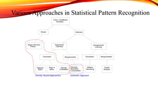
• Statistical pattern recognition
• Parameter Estimation Methods
• Principle Componenet Analysis
• Linear Discrimination Analysis
• Classification Techniques
• Nearest Neighbour rule and Bayes Classifier
• K-Means clustering
• Support Vector Machine
6.
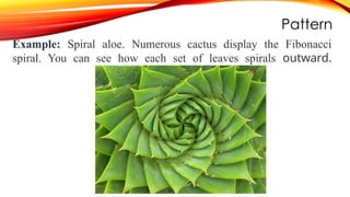
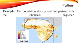
Pattern
Pattern is everythingaround in this digital world. A pattern can
either be seen physically or it can be observed mathematically by
applying algorithms.
Example: Angelica flowerhead, a sphere made of spheres
Pattern Recognition
• Patternrecognition is the process of recognizing patterns using a machine
learning algorithm. Pattern recognition is the classification of data based on
knowledge already gained or statistical information extracted from patterns
and/or their representation. One of the important aspects of pattern
recognition is its application potential.
• Examples: Speech recognition, speaker identification, multimedia document
recognition (MDR), automatic medical diagnosis.
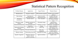
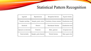
20.
Pattern Recognition
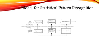
• Ina typical pattern recognition application, the raw data is processed and
converted into a form that is amenable for a machine to use. Pattern
recognition involves the classification and cluster of patterns.
• In classification, an appropriate class label is assigned to a pattern based on
an abstraction that is generated using a set of training patterns or domain
knowledge. Classification is used in supervised learning.
• Clustering generated a partition of the data which helps decision making, the
specific decision-making activity of interest to us. Clustering is used in
unsupervised learning.
21.
Pattern Recognition
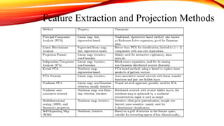
• Featuresmay be represented as continuous, discrete, or discrete binary
variables. A feature is a function of one or more measurements, computed so
that it quantifies some significant characteristics of the object.
• Example: consider our face then eyes, ears, nose, etc are features of the face.
A set of features that are taken together, forms the features vector.
• Example: In the above example of a face, if all the features (eyes, ears, nose,
etc) are taken together then the sequence is a feature vector([eyes, ears, nose]).
The feature vector is the sequence of a feature represented as a d-dimensional
column vector. In the case of speech, MFCC (Mel-frequency Cepstral
Coefficient) is the spectral feature of the speech. The sequence of the first 13
features forms a feature vector.
22.
Pattern Recognition
• Patternrecognition possesses the following features:
• Pattern recognition system should recognize familiar patterns quickly and
accurate
• Recognize and classify unfamiliar objects
• Accurately recognize shapes and objects from different angles
• Identify patterns and objects even when partly hidden
• Recognize patterns quickly with ease, and with automaticity.
23.
Pattern Recognition
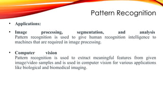
• Applications:
•Image processing, segmentation, and analysis
Pattern recognition is used to give human recognition intelligence to
machines that are required in image processing.
• Computer vision
Pattern recognition is used to extract meaningful features from given
image/video samples and is used in computer vision for various applications
like biological and biomedical imaging.
24.
Pattern Recognition
• Applications:
•Speech recognition
The greatest success in speech recognition has been obtained using pattern
recognition paradigms. It is used in various algorithms of speech recognition
which tries to avoid the problems of using a phoneme level of description
and treats larger units such as words as pattern
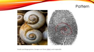
• Fingerprint identification
Fingerprint recognition technology is a dominant technology in the biometric
market. A number of recognition methods have been used to perform
fingerprint matching out of which pattern recognition approaches are widely
used.
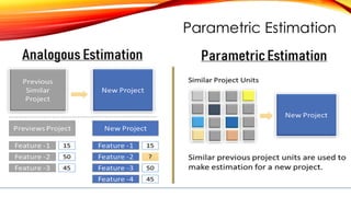
Parametric Estimation
• Parameterestimation is all about figuring out the unknown values in a
mathematical model based on data we have collected. In parameter
estimation, we use sample data to estimate a larger population's
characteristics (parameters).
• For instance, if a factory produces thousands of electronic components,
instead of testing each item, quality control teams might randomly sample a
certain number of items (e.g., 100 components) and check how many are
defective. If they find that 4 out of 100 components are defective, they can
estimate the proportion of defective items in the entire production batch as
4%.
34.
Parametric Estimation
• Typesof Parameter Estimation
• Parameter estimation generally falls into two types:
• Point Estimation
• Interval Estimation
35.
Point Estimation
• Pointestimation provides a single best guess of a parameter's
value.
• The result is one number that is considered the best
approximation of the population parameter based on the
sample data.
• For example, if we want to estimate the average height of
students in a school, the sample mean (average), we
calculate from a group of students serves as the point
estimate of the population mean.
36.
Interval Estimation
• Intervalestimation provides a range of values within which the
true parameter likely falls. This is more informative than point
estimation because it includes a measure of uncertainty.
• The range is known as a confidence interval, and it is
associated with a confidence level (often 95% or 99%) which
indicates the degree of certainty that the interval contains the
population parameter.
• For instance, if we estimate that the average height of students
in a school is between 150 cm and 160 cm with 95%
confidence, it means that we are 95% sure that the true
population mean lies within this interval.
37.
Methods of ParameterEstimation
There are various methods for estimating parameters, each suited for different
types of data and situations.
• Maximum Likelihood Estimation (MLE)
• Method of Moments
• Bayesian Estimation
• Principle Component Analysis
• Linear Discrimination Analysis
38.
Maximum Likelihood Estimation
•MLE is one of the most popular and widely used methods of parameter
estimation. The idea behind MLE is to find the parameter values that
maximize the likelihood function, which represents the probability of
observing the given sample data.
• The parameter value that maximizes the likelihood function is considered
the best estimate.
• MLE works well for large sample sizes and has desirable statistical properties,
such as being consistent (the estimate gets closer to the true value as the
sample size increases).
39.
Method of Moments
•The method of moments is a simpler, less computationally intense approach
than MLE.
• It is based on the idea that sample moments (such as the sample mean,
variance, etc.) can be used to estimate the population moments (such as the
population mean, variance, etc.).
• While not as precise as MLE, the method of moments is often easier to apply,
especially for small datasets.
40.
Bayesian Estimation
• Bayesianestimation is based on Bayes' theorem, which updates prior beliefs
about a parameter using observed data.
• In this method, we start with a "prior" distribution that reflects our initial
beliefs about the parameter. Then, as we gather sample data, we use Bayes'
theorem to calculate a "posterior" distribution, which combines the prior
information with the new data.
• Bayesian estimation is highly flexible and allows for incorporating external
information or expert knowledge into the estimation process. However, it
requires more complex computations, especially for large datasets.
41.
Principle Component Analysis
•Principal Component Analysis is an unsupervised learning algorithm that is
used for the dimensionality reduction in machine learning.
• It is a statistical process that converts the observations of correlated features
into a set of linearly uncorrelated features with the help of orthogonal
transformation. These new transformed features are called the Principal
Components.
• It is a technique to draw strong patterns from the given dataset by reducing
the variances.
• PCA generally tries to find the lower-dimensional surface to project the high-
dimensional data
42.
Principle Component Analysis
•Some common terms used in PCA algorithm:
• Dimensionality: It is the number of features or variables present in the given
dataset. More easily, it is the number of columns present in the dataset.
• Correlation: It signifies that how strongly two variables are related to each other.
Such as if one changes, the other variable also gets changed. The correlation value
ranges from -1 to +1. Here, -1 occurs if variables are inversely proportional to each
other, and +1 indicates that variables are directly proportional to each other.
• Orthogonal: It defines that variables are not correlated to each other, and hence
the correlation between the pair of variables is zero.
• Eigenvectors: If there is a square matrix M, and a non-zero vector v is given. Then
v will be eigenvector if Av is the scalar multiple of v.
• Covariance Matrix: A matrix containing the covariance between the pair of
variables is called the Covariance Matrix.
43.
Principle Component Analysis
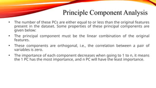
•The number of these PCs are either equal to or less than the original features
present in the dataset. Some properties of these principal components are
given below:
• The principal component must be the linear combination of the original
features.
• These components are orthogonal, i.e., the correlation between a pair of
variables is zero.
• The importance of each component decreases when going to 1 to n, it means
the 1 PC has the most importance, and n PC will have the least importance.
44.
Steps of PrincipleComponent Analysis
• Getting the dataset
Firstly, we need to take the input dataset and divide it into two subparts X and Y, where X is the
training set, and Y is the validation set.
• Representing data into a structure
Now we will represent our dataset into a structure. Such as we will represent the two-dimensional
matrix of independent variable X. Here each row corresponds to the data items, and the column
corresponds to the Features. The number of columns is the dimensions of the dataset.
• Standardizing the data
In this step, we will standardize our dataset. Such as in a particular column, the features with high
variance are more important compared to the features with lower variance.
If the importance of features is independent of the variance of the feature, then we will divide each
data item in a column with the standard deviation of the column. Here we will name the matrix as
Z.
• Calculating the Covariance of Z
To calculate the covariance of Z, we will take the matrix Z, and will transpose it. After transpose, we
will multiply it by Z. The output matrix will be the Covariance matrix of Z.
45.
Steps of PrincipleComponent Analysis
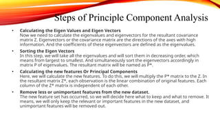
• Calculating the Eigen Values and Eigen Vectors
Now we need to calculate the eigenvalues and eigenvectors for the resultant covariance
matrix Z. Eigenvectors or the covariance matrix are the directions of the axes with high
information. And the coefficients of these eigenvectors are defined as the eigenvalues.
• Sorting the Eigen Vectors
In this step, we will take all the eigenvalues and will sort them in decreasing order, which
means from largest to smallest. And simultaneously sort the eigenvectors accordingly in
matrix P of eigenvalues. The resultant matrix will be named as P*.
• Calculating the new features Or Principal Components
Here, we will calculate the new features. To do this, we will multiply the P* matrix to the Z. In
the resultant matrix Z*, each observation is the linear combination of original features. Each
column of the Z* matrix is independent of each other.
• Remove less or unimportant features from the new dataset.
The new feature set has occurred, so we will decide here what to keep and what to remove. It
means, we will only keep the relevant or important features in the new dataset, and
unimportant features will be removed out.
46.
Linear Discrimination Analysis
•Linear Discriminant Analysis (LDA), also known as Normal Discriminant Analysis or
Discriminant Function Analysis, is a dimensionality reduction technique primarily
utilized in supervised classification problems.
• It facilitates the modeling of distinctions between groups, effectively separating
two or more classes.
• LDA operates by projecting features from a higher-dimensional space into a
lower-dimensional one.
• In machine learning, LDA serves as a supervised learning algorithm specifically
designed for classification tasks, aiming to identify a linear combination of
features that optimally segregates classes within a dataset.
47.
Linear Discrimination Analysis
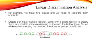
•For example, we have two classes and we need to separate them
efficiently.
• Classes can have multiple features. Using only a single feature to classify
them may result in some overlapping as shown in the below figure. So, we
will keep on increasing the number of features for proper classification.
48.
Working of LDA
•LDA works by projecting the data onto a lower-dimensional
space that maximizes the separation between the classes.
• It does this by finding a set of linear discriminants that
maximize the ratio of between-class variance to within-class
variance.
• In other words, it finds the directions in the feature space that
best separates the different classes of data.
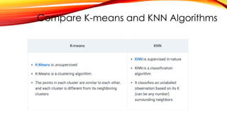
What is Classification?
•In short, classification is a form of “pattern recognition,” with
classification algorithms applied to the training data to find the
same pattern (similar words or sentiments, number sequences,
etc.) in future sets of data.
• Using classification algorithms, text analysis software can
perform tasks like aspect-based sentiment analysis to categorize
unstructured text by topic and polarity of opinion (positive,
negative, neutral, and beyond).
54.
What is Classification?
•Classification is the process of recognizing, understanding, and
grouping ideas and objects into preset categories or “sub-populations.”
Using pre-categorized training datasets, machine learning programs
use a variety of algorithms to classify future datasets into categories.
• Classification algorithms in machine learning use input training data to
predict the likelihood that subsequent data will fall into one of the
predetermined categories. One of the most common uses of
classification is filtering emails into “spam” or “non-spam.”
55.
Top 3 ClassificationAlgorithms in Machine Learning
● Naive Bayes
● K-Nearest Neighbors
● Support Vector Machines
K-nearest Neighbors
• K-nearestneighbors (k-NN) is a pattern recognition algorithm that
uses training datasets to find the k closest relatives in future
examples.
• When k-NN is used in classification, you calculate to place data within
the category of its nearest neighbor.
• If k = 1, then it would be placed in the class nearest 1. K is classified
by a plurality poll of its neighbors.
59.
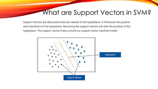
Support Vector Machines
•A support vector machine (SVM) uses
algorithms to train and classify data
within degrees of polarity, taking it to a
degree beyond X/Y prediction.
• For a simple visual explanation, we’ll
use two tags: red and blue, with two
data features: X and Y, then train our
classifier to output an X/Y coordinate
as either red or blue.
60.
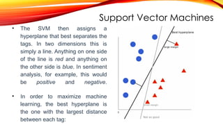
Support Vector Machines
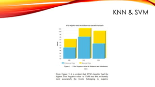
•The SVM then assigns a
hyperplane that best separates the
tags. In two dimensions this is
simply a line. Anything on one side
of the line is red and anything on
the other side is blue. In sentiment
analysis, for example, this would
be positive and negative.
• In order to maximize machine
learning, the best hyperplane is
the one with the largest distance
between each tag:
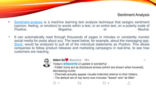
Sentiment Analysis
• Sentimentanalysis is a machine learning text analysis technique that assigns sentiment
(opinion, feeling, or emotion) to words within a text, or an entire text, on a polarity scale of
Positive, Negative, or Neutral.
• It can automatically read through thousands of pages in minutes or constantly monitor
social media for posts about you. The tweet below, for example, about the messaging app,
Slack, would be analyzed to pull all of the individual statements as Positive. This allows
companies to follow product releases and marketing campaigns in real-time, to see how
customers are reacting.
63.
Email Spam Classification
•One of the most common uses of classification, working non-stop and with
little need for human interaction, email spam classification saves us from
tedious deletion tasks and sometimes even costly phishing scams.
• Email applications use the above algorithms to calculate the likelihood that an
email is either not intended for the recipient or unwanted spam. Using text
analysis classification techniques, spam emails are weeded out from the
regular inbox: perhaps a recipient’s name is spelled incorrectly, or certain
scamming keywords are used.
• Spam classifiers do still need to be trained to a degree, as we’ve all
experienced when signing up for an email list of some sort that ends up in the
spam folder.
64.
Document Classification
• Documentclassification is the ordering of documents into categories
according to their content. This was previously done manually, as in the library
sciences or hand-ordered legal files. Machine learning classification
algorithms, however, allow this to be performed automatically.
• Document classification differs from text classification, in that, entire
documents, rather than just words or phrases, are classified. This is put into
practice when using search engines online, cross-referencing topics in legal
documents, and searching healthcare records by drug and diagnosis.
65.
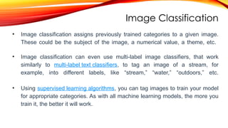
Image Classification
• Imageclassification assigns previously trained categories to a given image.
These could be the subject of the image, a numerical value, a theme, etc.
• Image classification can even use multi-label image classifiers, that work
similarly to multi-label text classifiers, to tag an image of a stream, for
example, into different labels, like “stream,” “water,” “outdoors,” etc.
• Using supervised learning algorithms, you can tag images to train your model
for appropriate categories. As with all machine learning models, the more you
train it, the better it will work.
66.
K-nearest Neighbors
• K-nearestneighbors (k-NN) is a pattern recognition algorithm that
uses training datasets to find the k closest relatives in future
examples.
• When k-NN is used in classification, you calculate to place data within
the category of its nearest neighbor.
• If k = 1, then it would be placed in the class nearest 1. K is classified
by a plurality poll of its neighbors.
67.
Explain the KNearest Neighbor Algorithm
• K nearest neighbor algorithm is a classification algorithm
that works in a way that a new data point is assigned to a
neighboring group to which it is most similar.
• In K nearest neighbors, K can be an integer greater than 1.
• So, for every new data point, we want to classify, we
compute to which neighboring group it is closest.
68.
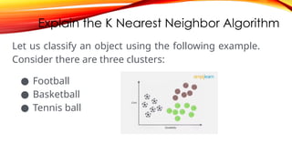
Explain the KNearest Neighbor Algorithm
Let us classify an object using the following example.
Consider there are three clusters:
● Football
● Basketball
● Tennis ball
69.
Explain the KNearest Neighbor Algorithm
● Let the new data point to be classified is a
black ball. We use KNN to classify it.
● Assume K = 5 (initially). Next, we find the K
(five) nearest data points.
● Observe that all five selected points do not
belong to the same cluster.
● There are three tennis balls and one each
of basketball and football.
● When multiple classes are involved, we
prefer the majority.
● Here the majority is with the tennis ball, so
the new data point is assigned to this
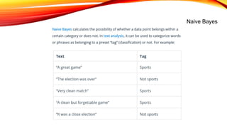
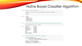
Naïve Bayes ClassifierAlgorithm
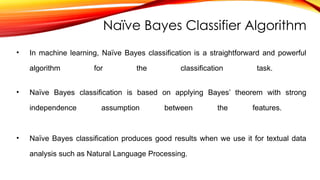
• In machine learning, Naïve Bayes classification is a straightforward and powerful
algorithm for the classification task.
• Naïve Bayes classification is based on applying Bayes’ theorem with strong
independence assumption between the features.
• Naïve Bayes classification produces good results when we use it for textual data
analysis such as Natural Language Processing.
75.
Naïve Bayes ClassifierAlgorithm
• Naïve Bayes models are also known as simple Bayes or independent Bayes.
• All these names refer to the application of Bayes’ theorem in the classifier’s decision
rule.
• Naïve Bayes classifier applies the Bayes’ theorem in practice.
• This classifier brings the power of Bayes’ theorem to machine learning.
76.
Naïve Bayes ClassifierAlgorithm
Naïve Bayes is one of the most straightforward and fast classification algorithm. It is
very well suited for large volume of data. It is successfully used in various applications
such as
1. Spam filtering
2. Text classification
3. Sentiment analysis
4. Recommender systems
It uses Bayes theorem of probability for prediction of unknown class.
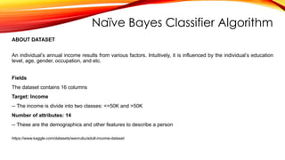
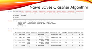
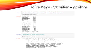
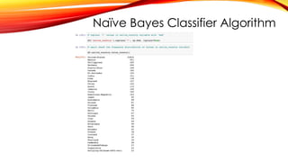
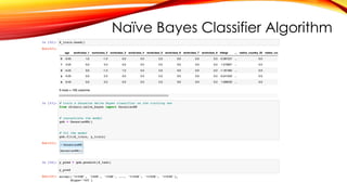
Naïve Bayes ClassifierAlgorithm
ABOUT DATASET
An individual’s annual income results from various factors. Intuitively, it is influenced by the individual’s education
level, age, gender, occupation, and etc.
Fields
The dataset contains 16 columns
Target: Income
-- The income is divide into two classes: <=50K and >50K
Number of attributes: 14
-- These are the demographics and other features to describe a person
https://www.kaggle.com/datasets/wenruliu/adult-income-dataset
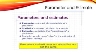
What Is ‘naive’in the Naive Bayes Classifier?
• The classifier is called ‘naive’ because it makes assumptions that
may or may not turn out to be correct.
• The algorithm assumes that the presence of one feature of a class
is not related to the presence of any other feature (absolute
independence of features), given the class variable.
• For instance, a fruit may be considered to be a cherry if it is red in
color and round in shape, regardless of other features. This
assumption may or may not be right (as an apple also matches the
description).
101.
Support Vector Machines
•A support vector machine (SVM) uses
algorithms to train and classify data
within degrees of polarity, taking it to a
degree beyond X/Y prediction.
• For a simple visual explanation, we’ll
use two tags: red and blue, with two
data features: X and Y, then train our
classifier to output an X/Y coordinate
as either red or blue.
102.
Support Vector Machines
•The SVM then assigns a
hyperplane that best separates the
tags. In two dimensions this is
simply a line. Anything on one side
of the line is red and anything on
the other side is blue. In sentiment
analysis, for example, this would
be positive and negative.
• In order to maximize machine
learning, the best hyperplane is
the one with the largest distance
between each tag:
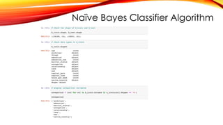
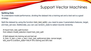
Support Vector Machines
#Import train_test_split function
from sklearn.model_selection import train_test_split
# Split dataset into training set and test set
X_train, X_test, y_train, y_test = train_test_split(cancer.data, cancer.target,
test_size=0.3,random_state=109) # 70% training and 30% test
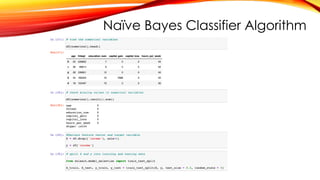
Splitting Data
To understand model performance, dividing the dataset into a training set and a test set is a good
strategy.
Split the dataset by using the function train_test_split(). you need to pass 3 parameters features, target,
and test_set size. Additionally, you can use random_state to select records randomly.


![Pattern Recognition
• Features may be represented as continuous, discrete, or discrete binary
variables. A feature is a function of one or more measurements, computed so
that it quantifies some significant characteristics of the object.
• Example: consider our face then eyes, ears, nose, etc are features of the face.
A set of features that are taken together, forms the features vector.
• Example: In the above example of a face, if all the features (eyes, ears, nose,
etc) are taken together then the sequence is a feature vector([eyes, ears, nose]).
The feature vector is the sequence of a feature represented as a d-dimensional
column vector. In the case of speech, MFCC (Mel-frequency Cepstral
Coefficient) is the spectral feature of the speech. The sequence of the first 13
features forms a feature vector.](https://image.slidesharecdn.com/kca301aiunit5patternrecognition-250331113543-aa9d54ee/85/AI-Unit-5-Pattern-Recognition-AKTU-pptx-21-320.jpg)