Advanced Methods and Deep Learning in Computer Vision (Computer Vision and Pattern Recognition) 1st Edition E. R. Davies
Advanced Methods and Deep Learning in Computer Vision (Computer Vision and Pattern Recognition) 1st Edition E. R. Davies
Advanced Methods and Deep Learning in Computer Vision (Computer Vision and Pattern Recognition) 1st Edition E. R. Davies


![1.1. Introduction – computer vision and its origins 3
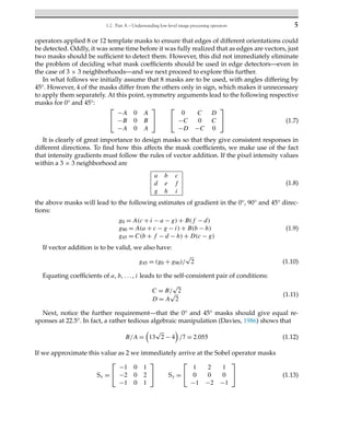
Both of these are linear convolution kernels, which by definition are spatially invariant
over the image space. A general 3 × 3 convolution mask is given by
⎡
⎣
c4 c3 c2
c5 c0 c1
c6 c7 c8
⎤
⎦ (1.2)
where the local pixels are assigned labels 0–8. Next, we take the intensity values in a local
3 × 3 image neighborhood as
P4 P3 P2
P5 P0 P1
P6 P7 P8
(1.3)
If we now use a notation based approximately on C ++, we can write the complete con-
volution procedure in the form:
for all pixels in image do {
Q0 = P0 ∗ c0 + P1 ∗ c1 + P2 ∗ c2 + P3 ∗ c3 + P4 ∗ c4
+ P5 ∗ c5 + P6 ∗ c6 + P7 ∗ c7 + P8 ∗ c8;
} (1.4)
So far we have concentrated on convolution masks, which are linear combinations of input
intensities: these contrast with nonlinear procedures such as thresholding, which cannot be
expressed as convolutions. In fact, thresholding is a very widely used technique, and can be
written in the form:
for all pixels in image do {
if (P0 < thresh)A0 = 1; else A0 = 0;
} (1.5)
This procedure converts a grey scale image in P-space into a binary image in A-space. Here it
is used to identify dark objects by expressing them as 1s on a background of 0s.
We end this section by presenting a complete procedure for median filtering within a 3 × 3
neighborhood:
for (i = 0; i <= 255; i + +) hist[i] = 0;
for all pixels in image do {
for (m = 0;m <= 8;m + +) hist[P[m]] + +;
i = 0; sum = 0;
while (sum < 5){
sum = sum + hist[i];
i = i + l;
}](https://image.slidesharecdn.com/26951-250313203158-086bbe68/85/Advanced-Methods-and-Deep-Learning-in-Computer-Vision-Computer-Vision-and-Pattern-Recognition-1st-Edition-E-R-Davies-25-320.jpg)
![4 1. The dramatically changing face of computer vision
Q0 = i − 1;
for (m = 0;m <= 8;m + +) hist[P[m]] = 0;
} (1.6)
The notation P[0] is intended to denote P0, and so on for P[1] to P[8]. Note that the me-
dian operation is computation intensive, so time is saved by only reinitializing the particular
histogram elements that have actually been used.
An important point about the procedures covered by Eqs. (1.4)–(1.6) is that they take their
input from one image space and output it to another image space—a process often described
as parallel processing—thereby eliminating problems relating to the order in which the indi-
vidual pixel computations are carried out.
Finally, the image smoothing algorithms given by Eqs. (1.1)–(1.4) all use 3 × 3 convolution
kernels, though much larger kernels can obviously be used: indeed, they can alternatively
be implemented by first converting to the spatial frequency domain and then systematically
eliminating high spatial frequencies, albeit with an additional computational burden. On the
other hand, nonlinear operations such as median filtering cannot be tackled in this way.
For convenience, the remainder of this chapter has been split into a number of parts, as
follows:
Part A – Understanding low-level image processing perators
Part B – 2-D object location and recognition
Part C – 3-D object location and the importance of invariance
Part D – Tracking moving objects
Part E – Texture analysis
Part F – From artificial neural networks to deep learning methods
Part G – Summary.
Overall, the purpose of this chapter is to summarize vital parts of the early—or ‘legacy’—work
on computer vision, and to remind readers of their significance, so that they can more confi-
dently get to grips with recent advanced developments in the subject. However, the need to
make this sort of selection means that many other important topics have had to be excluded.
1.2 Part A – Understanding low-level image processing operators
1.2.1 The basics of edge detection
No imaging operation is more important or more widely used than edge detection. There
are important reasons for this, but ultimately, describing object shapes by their boundaries
and internal contours reduces the amount of data required to hold an N × N image from
O(N2) to O(N), thereby making subsequent storage and processing more efficient. Further-
more, there is much evidence that humans can recognize objects highly effectively, or even
with increased efficiency, from their boundaries: the quick responses humans can make from
2-D sketches and cartoons support this idea.
In the 1960s and 1970s, a considerable number of edge detection operators were developed,
many of them intuitively, which meant that their optimality was in question. A number of the](https://image.slidesharecdn.com/26951-250313203158-086bbe68/85/Advanced-Methods-and-Deep-Learning-in-Computer-Vision-Computer-Vision-and-Pattern-Recognition-1st-Edition-E-R-Davies-26-320.jpg)
![6 1. The dramatically changing face of computer vision
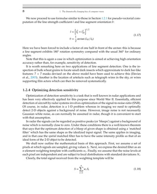
application of which yields maps of the gx, gy components of intensity gradient. As edges
are vectors, we can compute the local edge magnitude g and direction θ using the standard
vector-based formulae:
g =
g2
x + g2
y
1/2
θ = arctan gy/gx
(1.14)
Notice that whole-image calculations of g and θ will not be convolutions as they involve
nonlinear operations.
In summary, in Sections 1.1 and 1.2.1 we have described various categories of image pro-
cessing operator, including linear, nonlinear and convolution operators. Examples of (linear)
convolutions are mean and Gaussian smoothing and edge gradient component estimation.
Examples of nonlinear operations are thresholding, edge gradient and edge orientation com-
putations. Above all, it should be noted that the Sobel mask coefficients have been arrived at
in a principled (non ad hoc) way. In fact, they were designed to optimize accuracy of edge ori-
entation. Note also that, as we shall see later, orientation accuracy is of paramount importance
when edge information is passed to object location schemes such as the Hough transform.
1.2.2 The Canny operator
The aim of the Canny edge detector was to be far more accurate than basic edge detectors
such as the Sobel, and it caused quite a stir when it was published in 1986 (Canny, 1986). To
achieve such increases in accuracy, a number of processes are applied in turn:
1. The image is smoothed using a 2-D Gaussian to ensure that the intensity field is a mathe-
matically well-behaved function.
2. The image is differentiated using two 1-D derivative functions, such as those of the Sobel,
and the gradient magnitude field is computed.
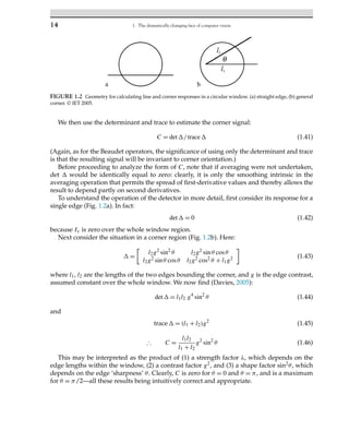
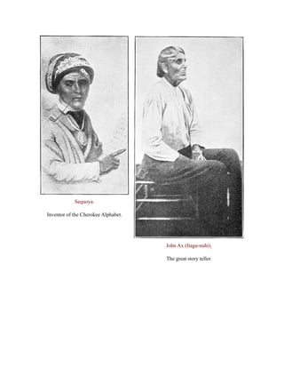
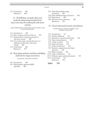
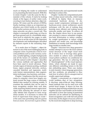
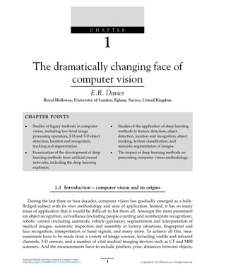
3. Nonmaximum suppression is employed along the local edge normal direction to thin the
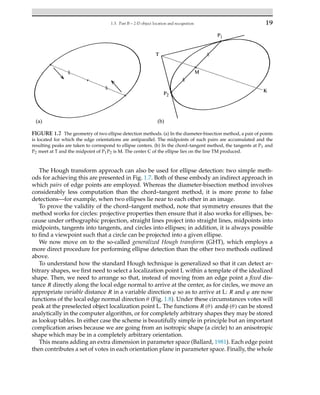
edges: this takes place in two stages (1) finding the two noncentral red points shown in
Fig. 1.1, which involves gradient magnitude interpolation between two pairs of pixels;
(2) performing quadratic interpolation between the intensity gradients at the three red
points to determine the position of the peak edge signal to subpixel precision.
4. ‘Hysteresis’ thresholding is performed: this involves applying two thresholds t1 and t2
(t2 t1) to the intensity gradient field; the result is ‘nonedge’ if g t1, ‘edge’ if g t2, and
otherwise is only ‘edge’ if next to ‘edge’. (Note that the ‘edge’ property can be propagated
from pixel to pixel under the above rules.)
As noted in item 3, quadratic interpolation can be used to locate the position of the gra-
dient magnitude peak. A few lines of algebra shows that, for the g-values g1, g2, g3 of
the three red points, the displacement of the peak from the central red point is equal to
(g3 − g1)secθ/[2(2g2 − g1 − g3)]: here, sec θ is the factor by which θ increases the distance
between the outermost red points.](https://image.slidesharecdn.com/26951-250313203158-086bbe68/85/Advanced-Methods-and-Deep-Learning-in-Computer-Vision-Computer-Vision-and-Pattern-Recognition-1st-Edition-E-R-Davies-28-320.jpg)
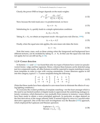
![10 1. The dramatically changing face of computer vision
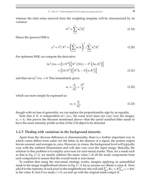
Overall, we should note that the zero-mean strategy is only an approximation, as there
will be places in an image where the background varies between high and low level, so that
zero-mean cancellation cannot occur exactly (i.e., B cannot be regarded as constant over the
region of the mask). Nevertheless, assuming that the background variation occurs on a scale
significantly larger than that of the mask size, this should work adequately.
It should be remarked that the zero-mean approximation is already widely used—as in-
deed we have already seen from the edge and line-segment masks in Eqs. (1.7) and (1.15). It
must also apply for other detectors we could devise, such as corner and hole detectors.
1.2.6 A theory combining the matched filter and zero-mean constructs
At first sight, the zero-mean construct is so simple that it might appear to integrate easily
with the matched filter formalism of Section 1.2.4. However, applying it reduces the number
of degrees of freedom of the matched filter by one, so a change is needed to the matched filter
formalism to ensure that the latter continues to be an ideal detector. To proceed, we represent
the zero-mean and matched filter cases as follows:
(wi)z-m = Si − S̄
(wi)m-f = Si/N2
i
(1.24)
Next, we combine these into the form
wi =
Si − S̃
/N2
i (1.25)
where we have avoided an impasse by trying a hypothetical (i.e., as yet unknown) type of
mean for S, which we call S̃. [Of course, if this hypothesis in the end results in a contradiction,
a fresh approach will naturally be required.] Applying the zero-mean condition
i wi = 0
now yields the following:
i
wi =
i
Si/N2
i −
i
S̃/N2
i = 0 (1.26)
∴ S̃
i
1/N2
i
=
i
Si/N2
i (1.27)
∴ S̃ =
i
Si/N2
i
/
i
1/N2
i
(1.28)
From this, we deduce that S̃ has to be a weighted mean, and in particular the noise-weighted
mean S̃. On the other hand, if the noise is uniform, S̃ will revert to the usual unweighted
mean S̄. Also, if we do not apply the zero-mean condition (which we can achieve by setting
S̃ = 0), Eq. (1.25) reverts immediately to the standard matched filter condition.
The formula for S̃ may seem to be unduly general, in that Ni should normally be almost
independent of i. However, if an ideal profile were to be derived by averaging real object
profiles, then away from its center, the noise variance could be more substantial. Indeed, for](https://image.slidesharecdn.com/26951-250313203158-086bbe68/85/Advanced-Methods-and-Deep-Learning-in-Computer-Vision-Computer-Vision-and-Pattern-Recognition-1st-Edition-E-R-Davies-32-320.jpg)