![Anomaly Detection for CMS
2
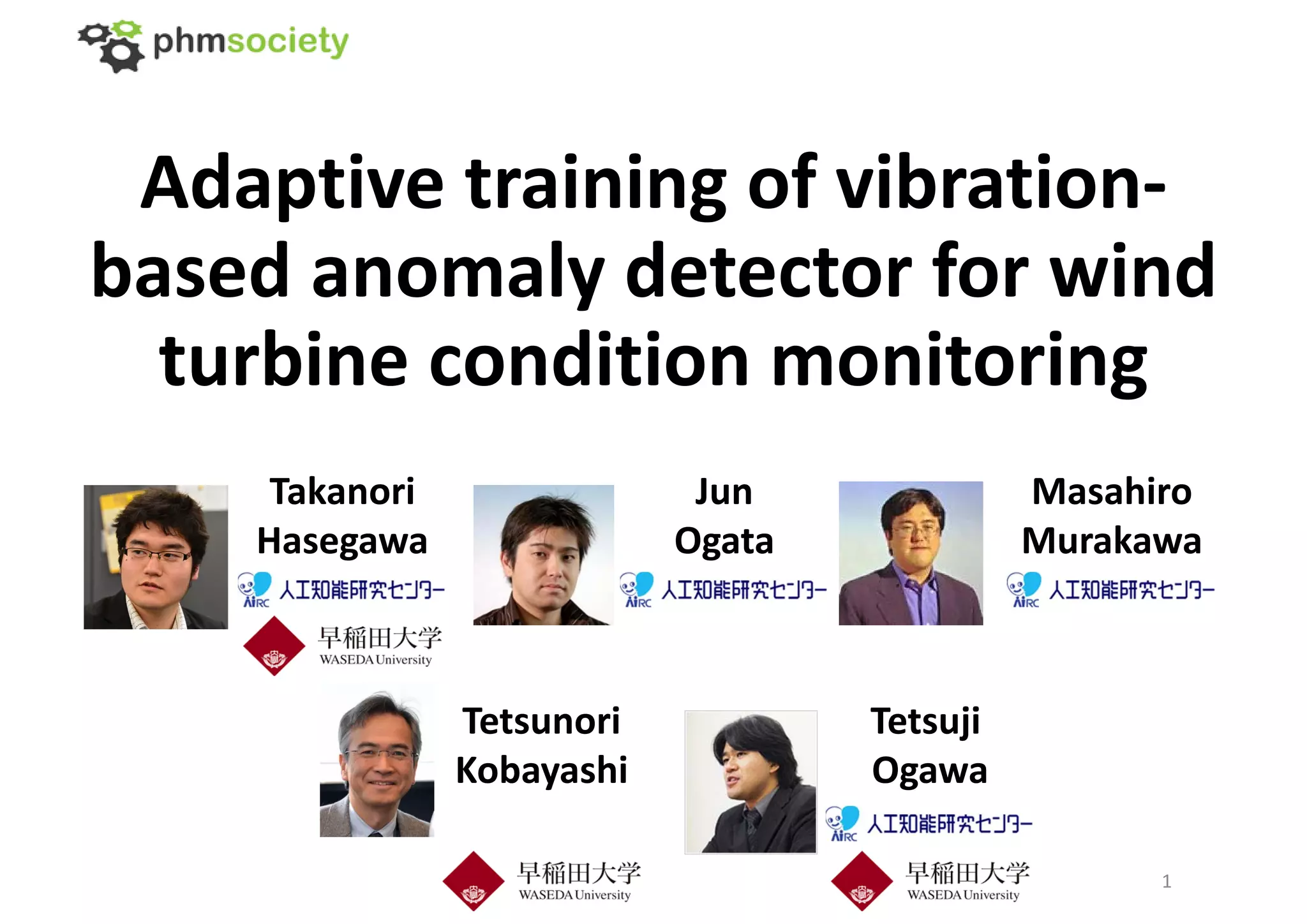
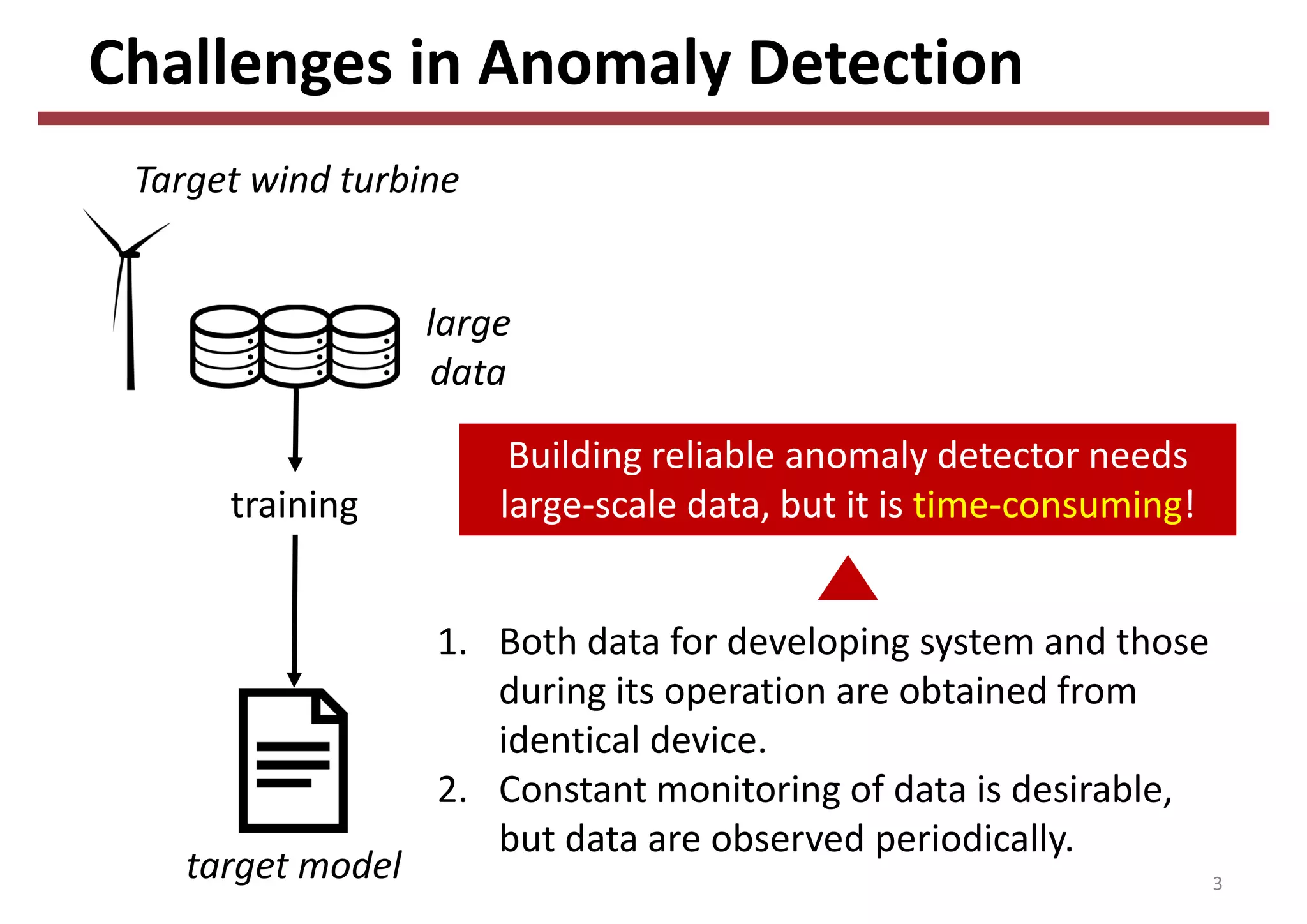
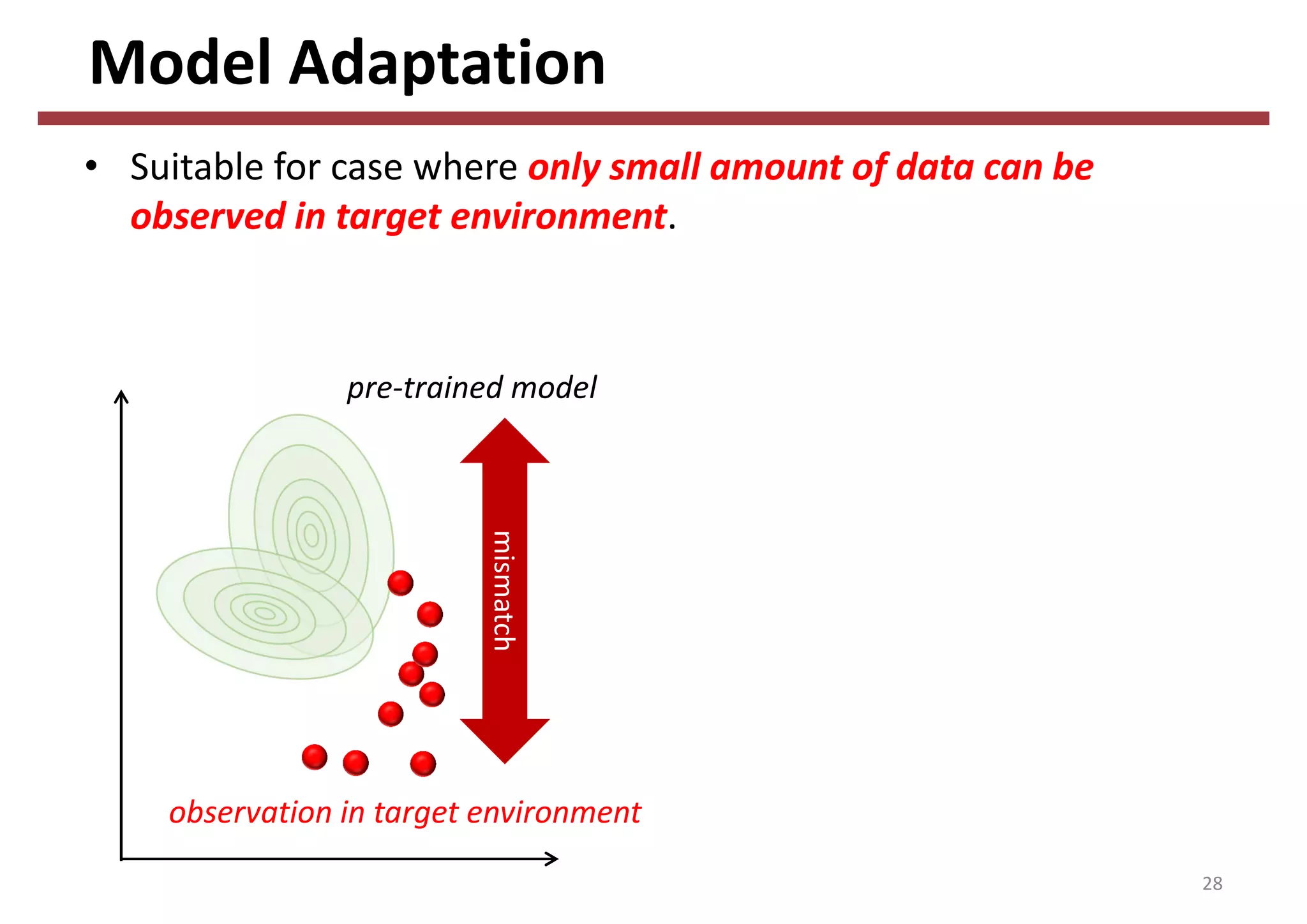
• Condition monitoring system (CMS) plays a vital role in
establishing condition‐based maintenance and repair (M&R).
• Anomaly (fault) detection is a key technology to realize effective
CMSs. [Afrooz, et al, 2014][A Zaher, et al, 2009][Z Hameed, et al 2009]
https://www.nrel.gov/continuum/partnering/wind.html](https://image.slidesharecdn.com/phm2017-slides-hasegawa-180512121142/75/Adaptive-training-of-vibration-based-anomaly-detector-for-wind-turbine-condition-monitoring-2-2048.jpg)


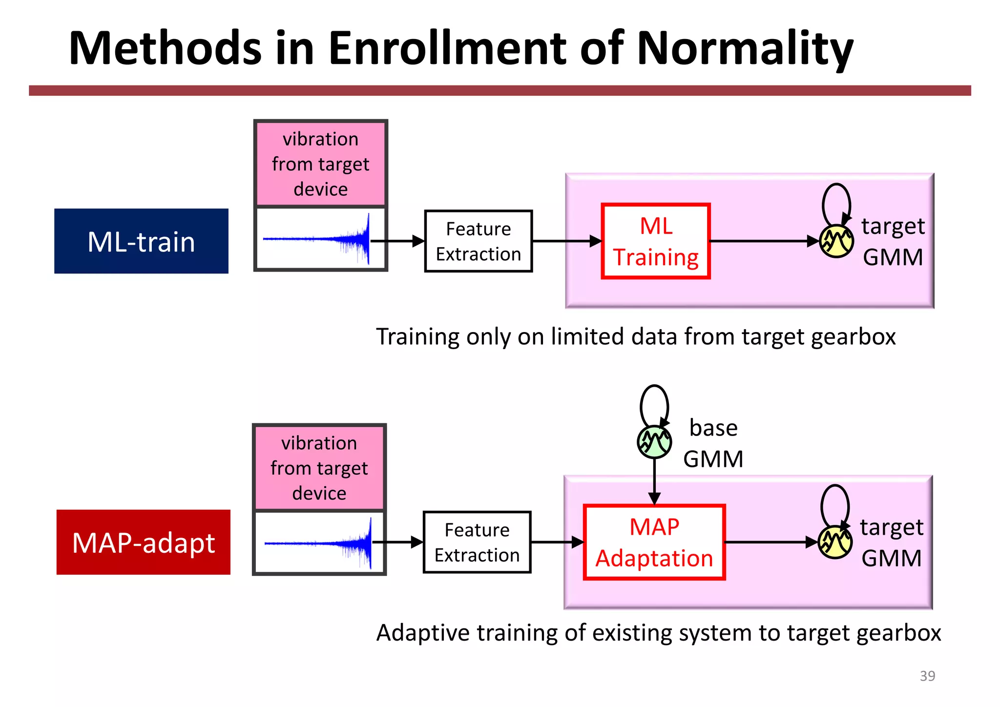
![MAP adaptation works on less training data
40
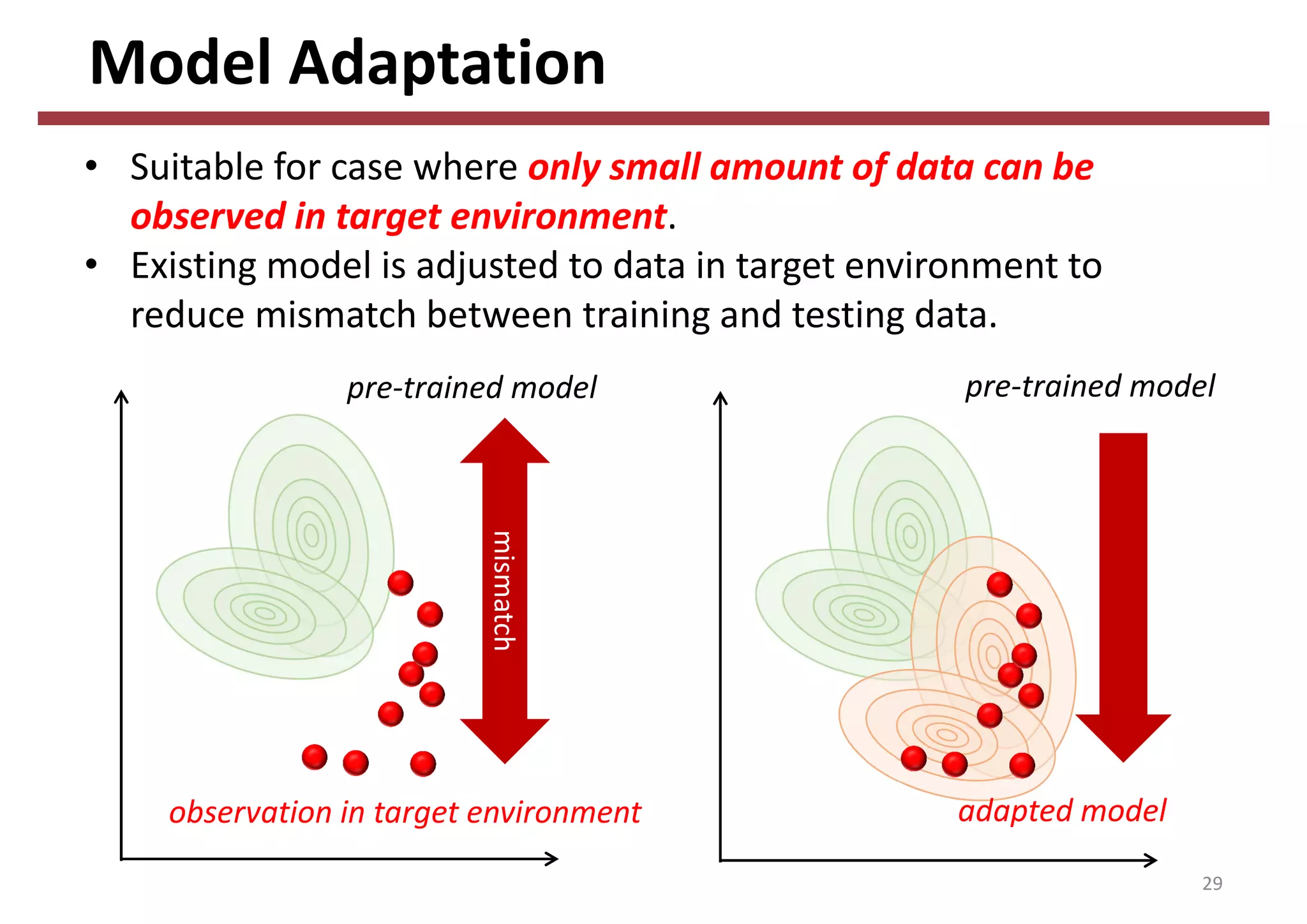
MAP adaptation successfully
reduces AUCs at early stage of
collecting data.
0.10
0.61
4132
AUC
Data length [frame]
590](https://image.slidesharecdn.com/phm2017-slides-hasegawa-180512121142/75/Adaptive-training-of-vibration-based-anomaly-detector-for-wind-turbine-condition-monitoring-40-2048.jpg)
![Advantages of MAP Adaptation
41
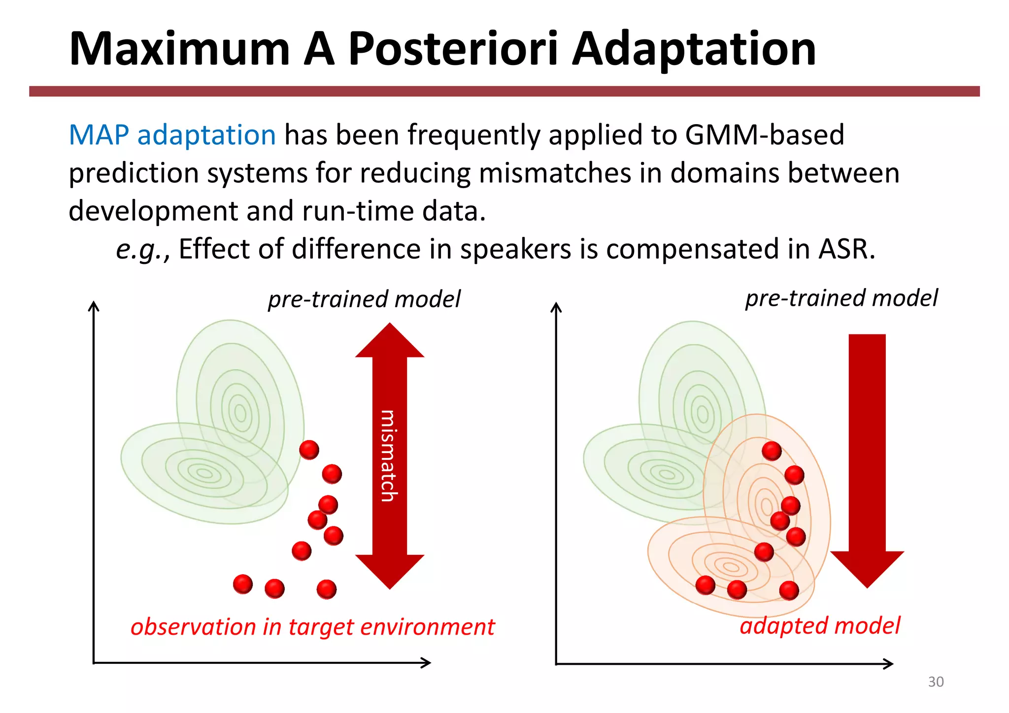
Adapted system can handle
initial failure owing to its high‐
performance at early stage of
monitoring.
4132
AUC
Data length [frame]
590](https://image.slidesharecdn.com/phm2017-slides-hasegawa-180512121142/75/Adaptive-training-of-vibration-based-anomaly-detector-for-wind-turbine-condition-monitoring-41-2048.jpg)

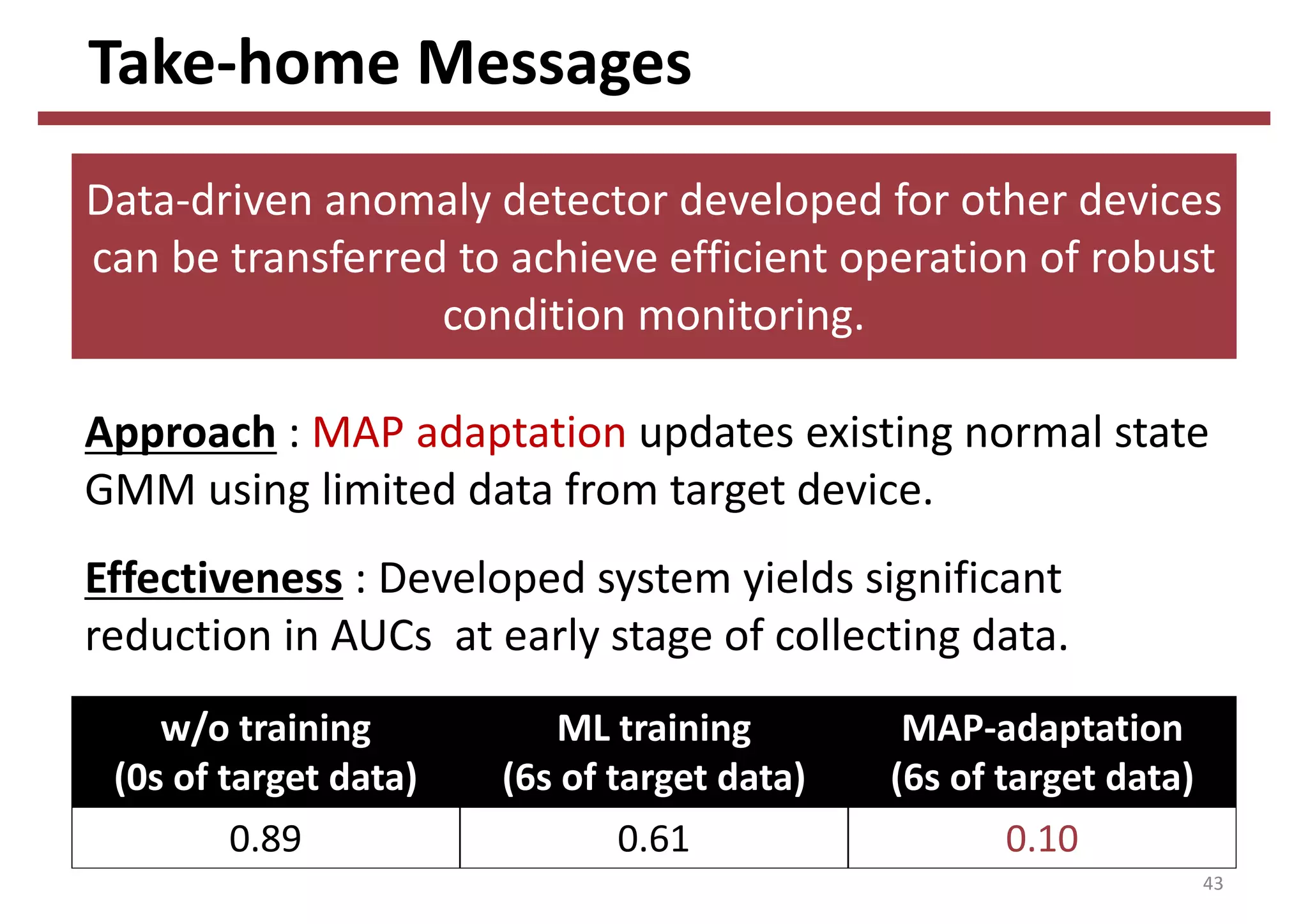

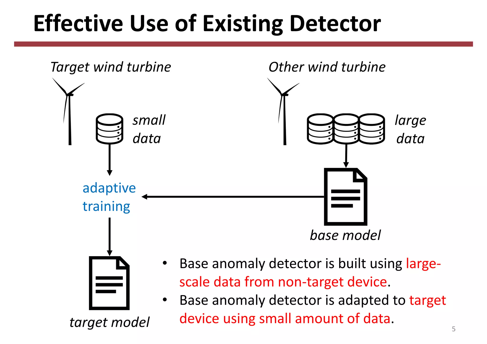
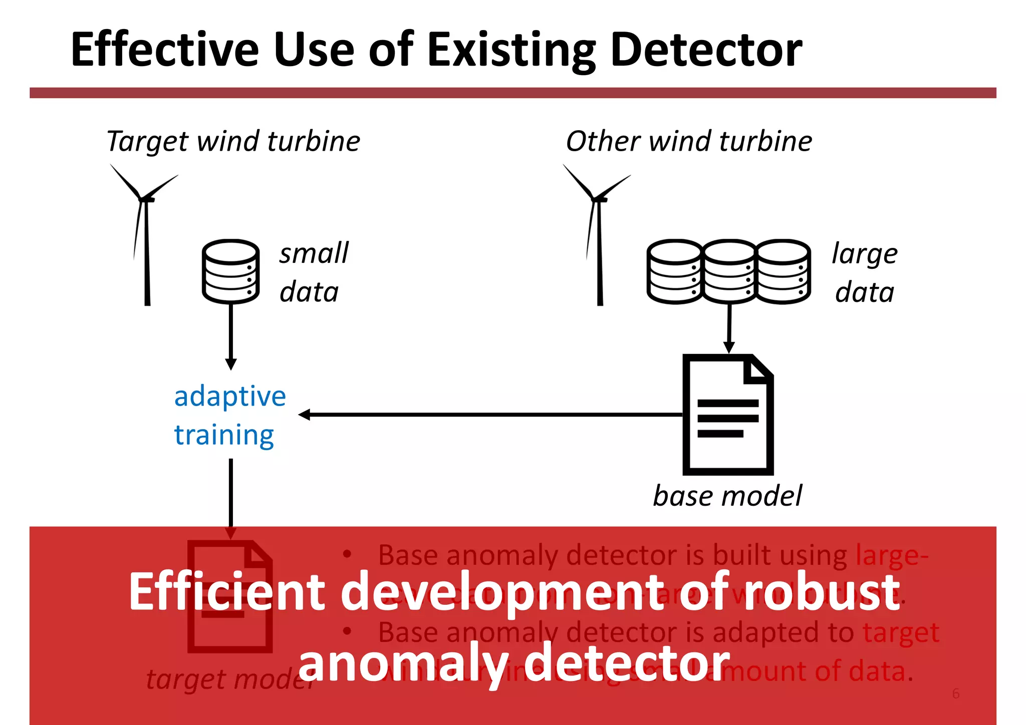
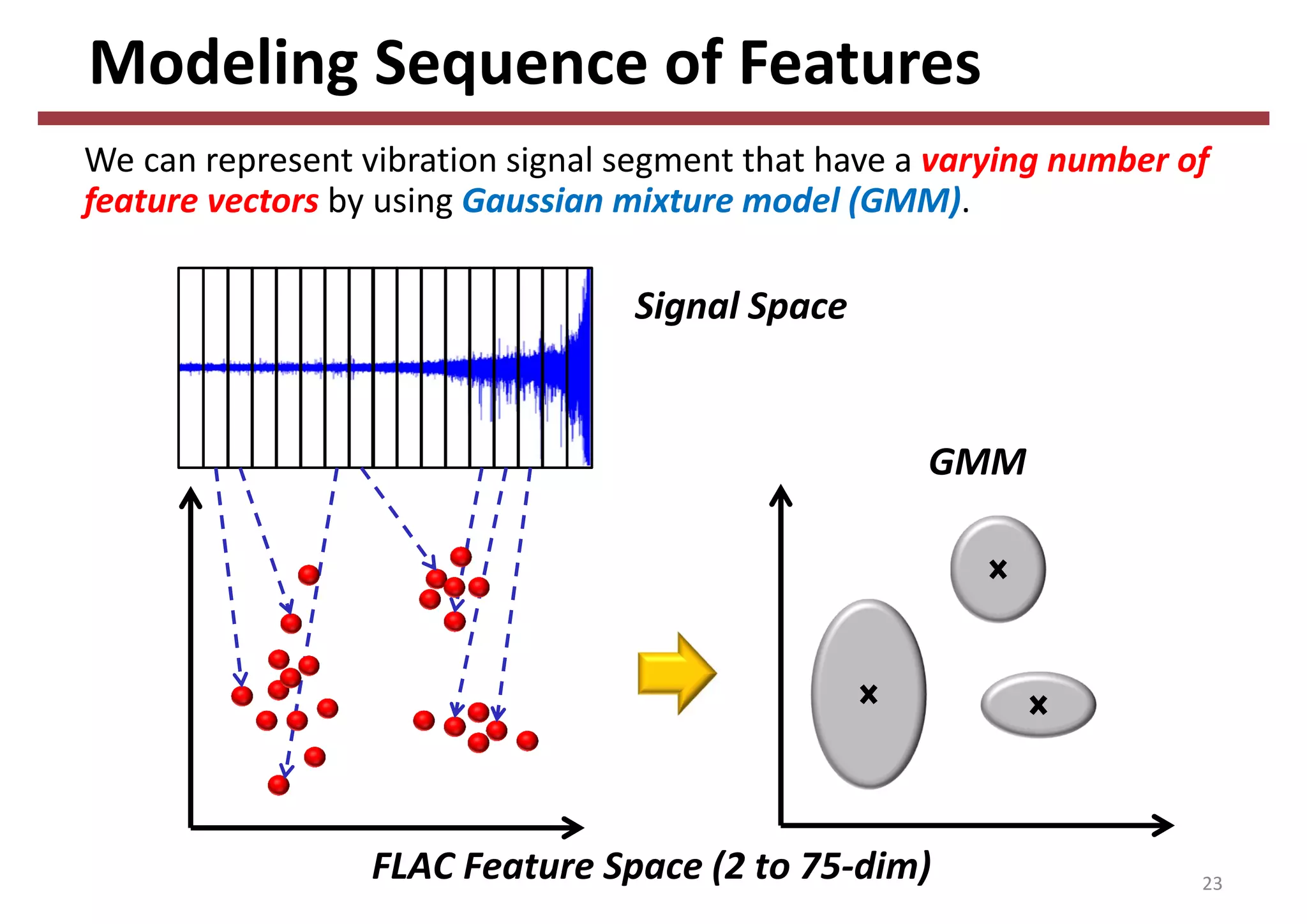
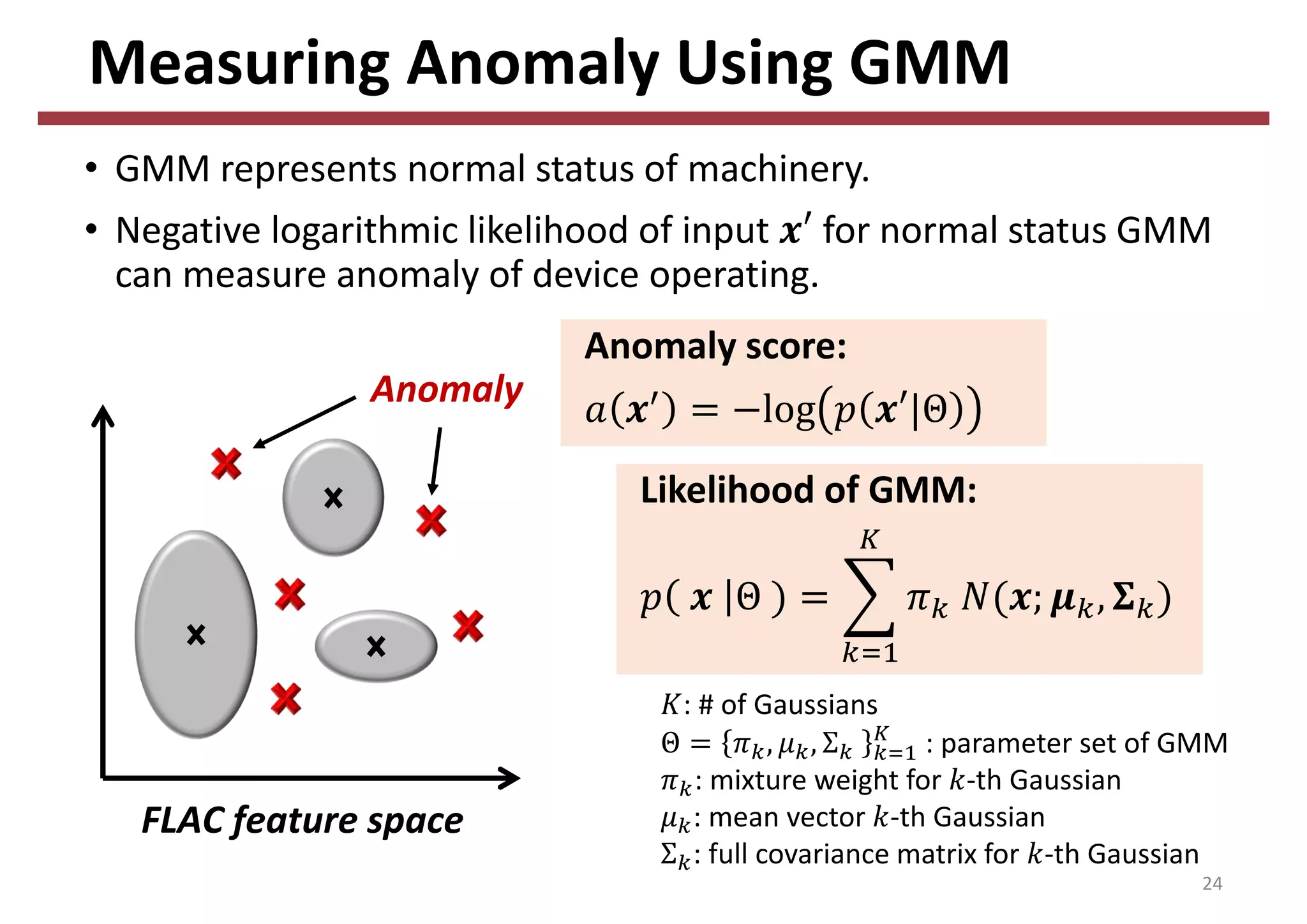
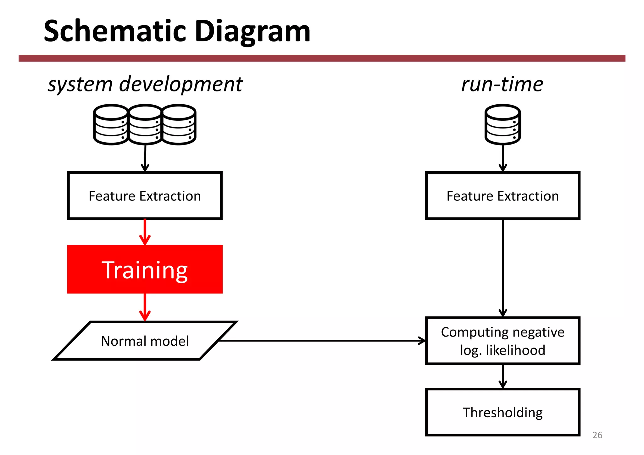
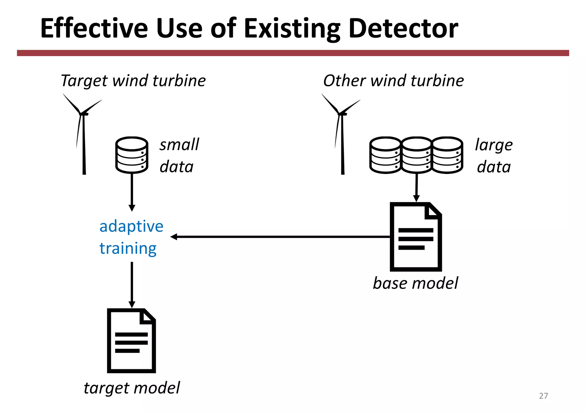
The document discusses the development of an adaptive training method for an anomaly detector used in wind turbine condition monitoring, emphasizing the challenges of limited data availability. It presents a gmm-based anomaly detection system that can be effectively adapted using a small amount of data from the target device while leveraging a pre-trained model. The results indicate that this adaptive approach significantly improves anomaly detection performance, especially in early stages of monitoring.