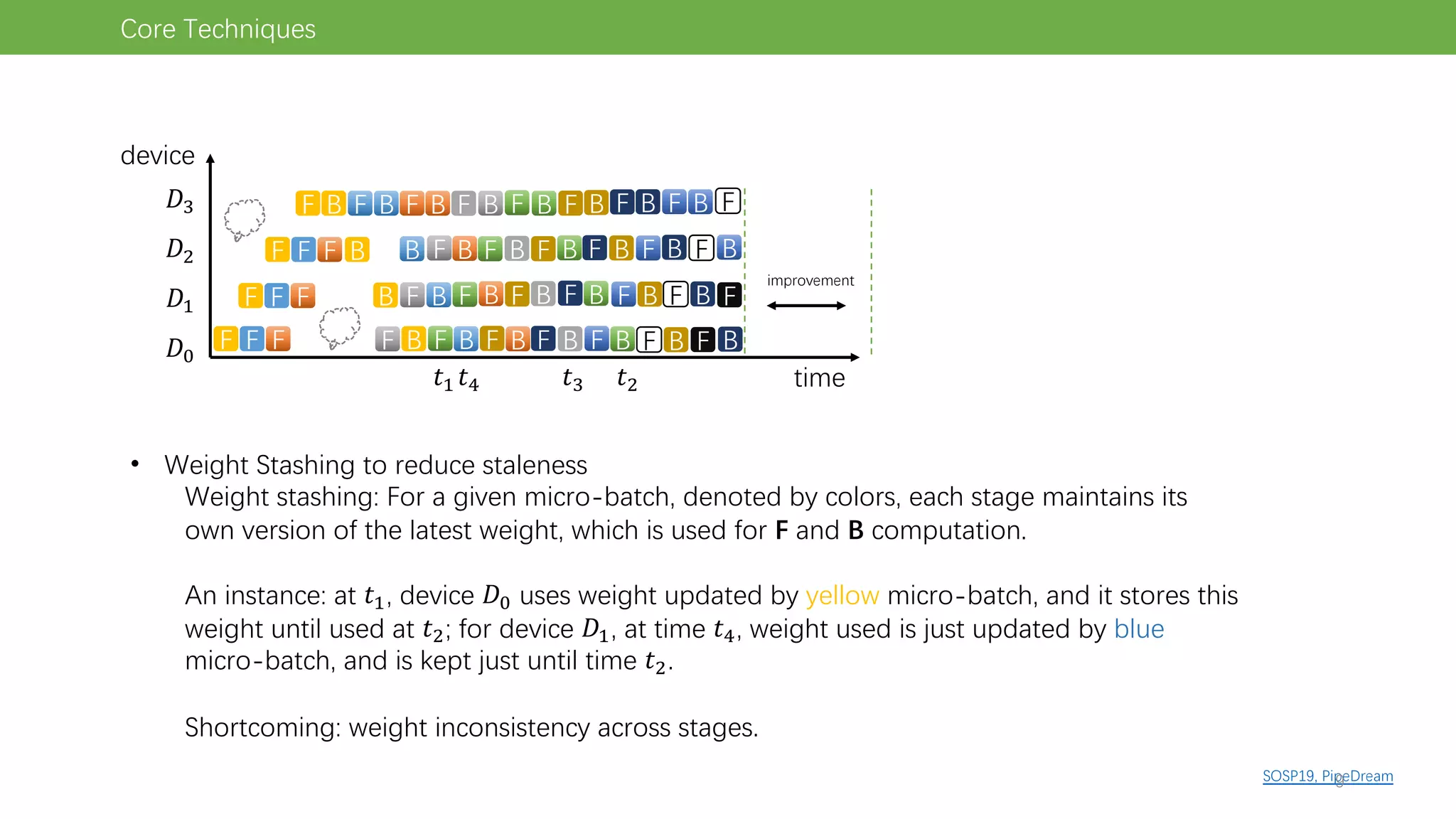
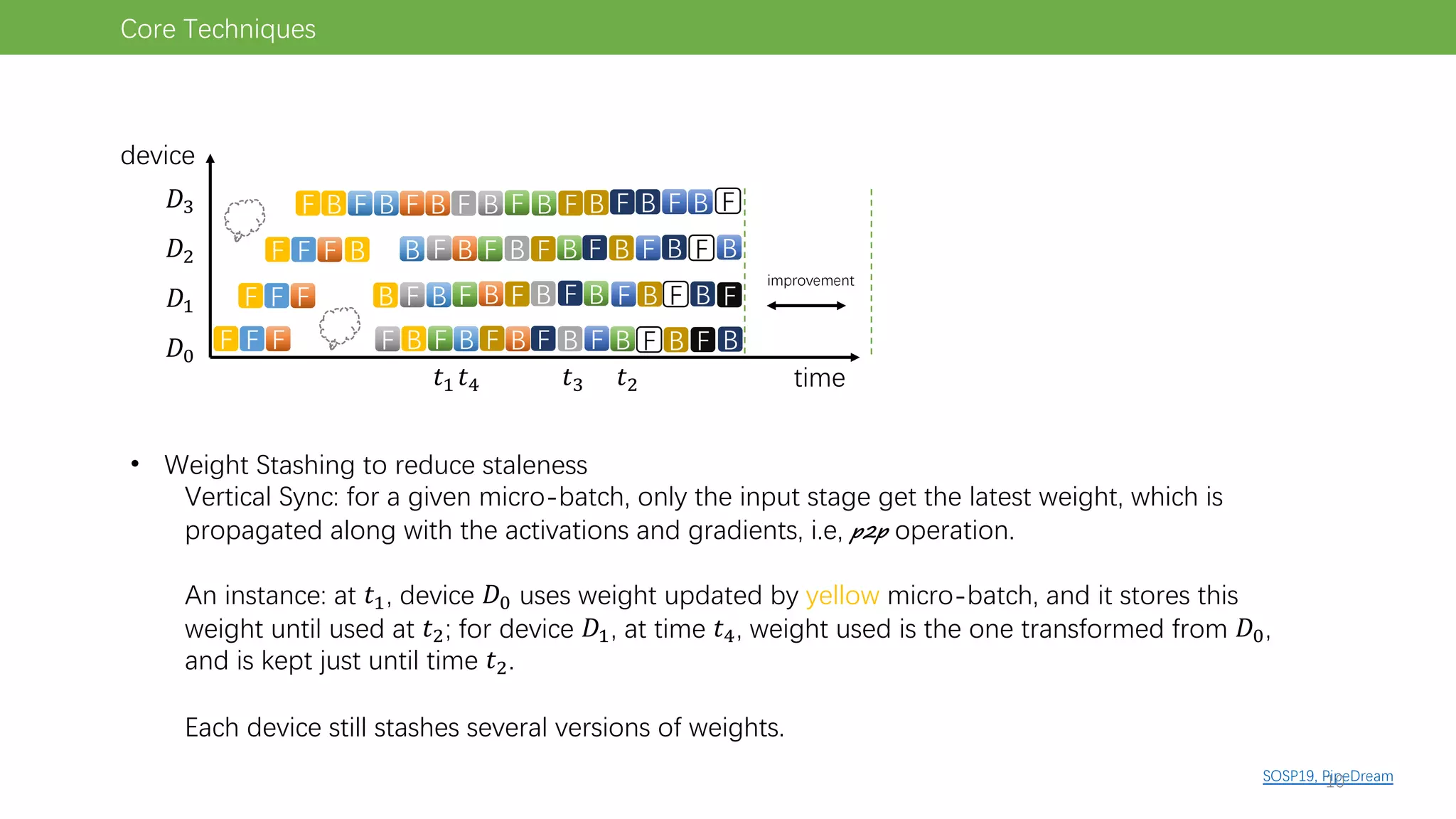
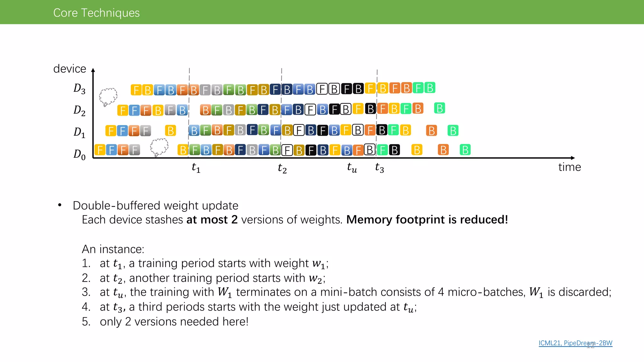
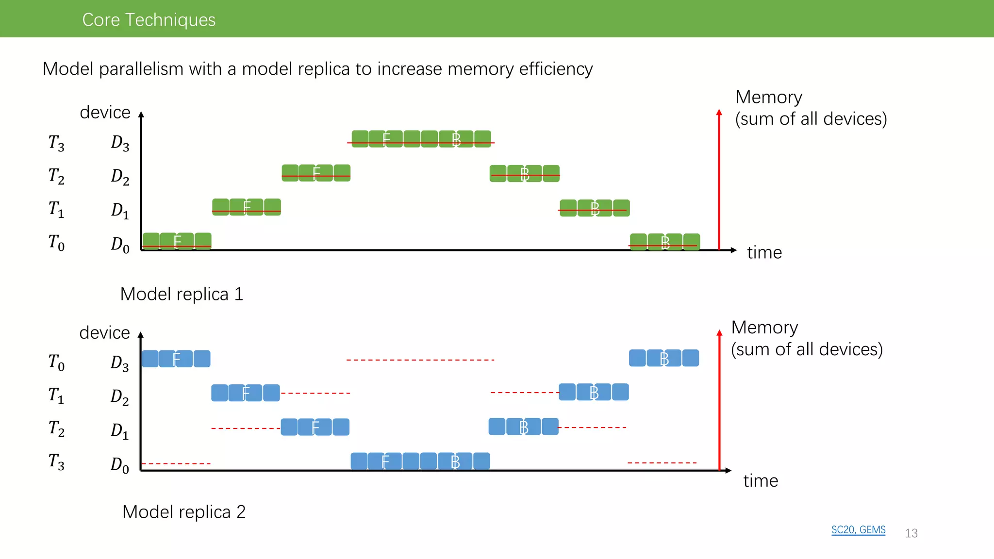
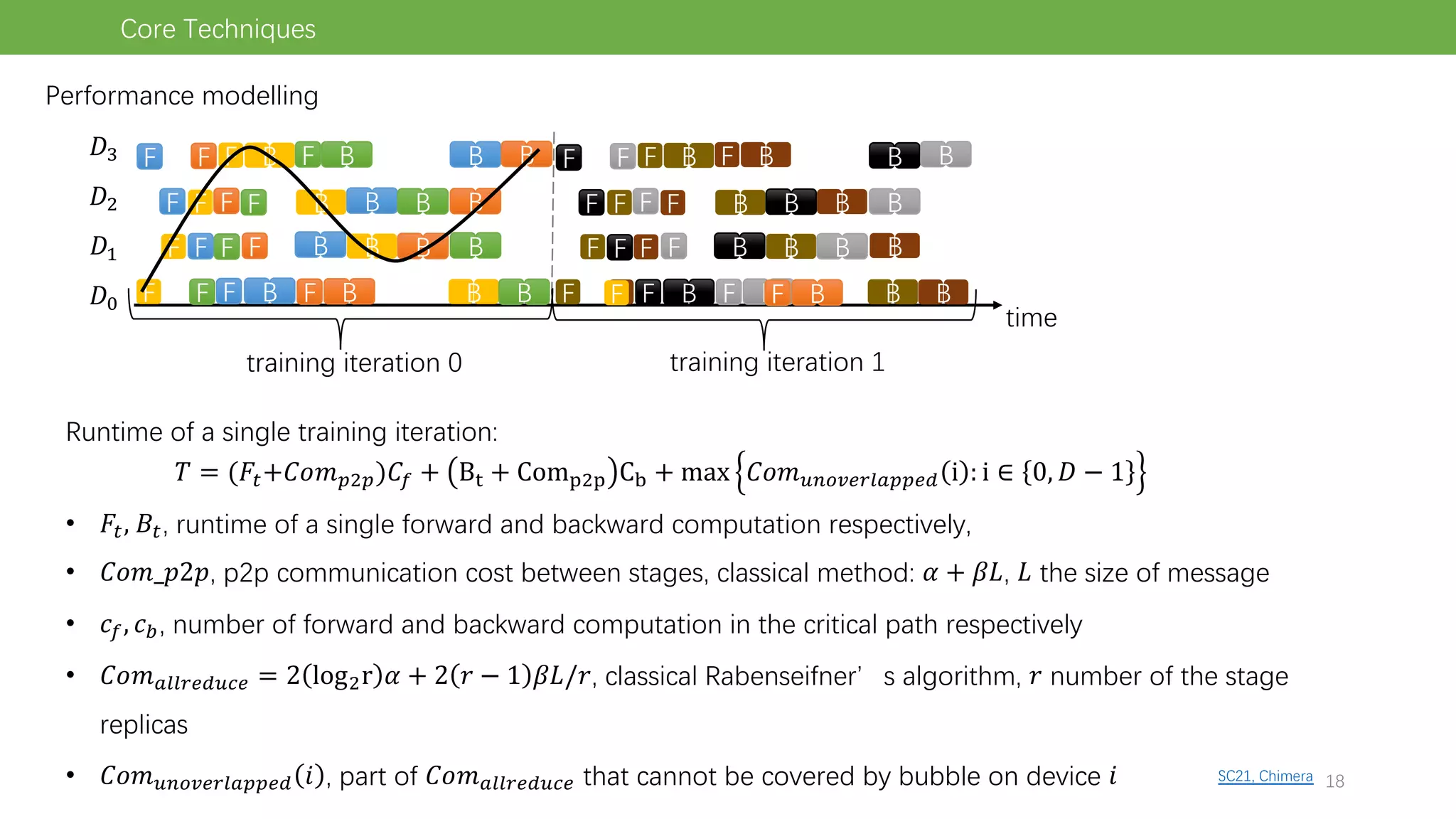
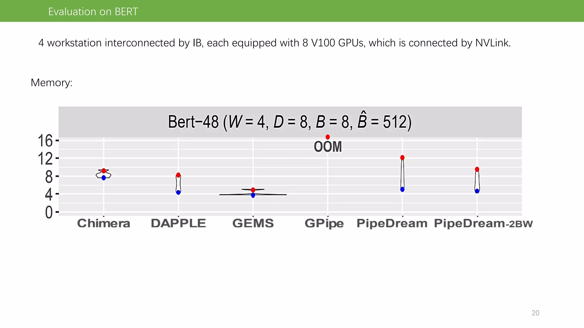
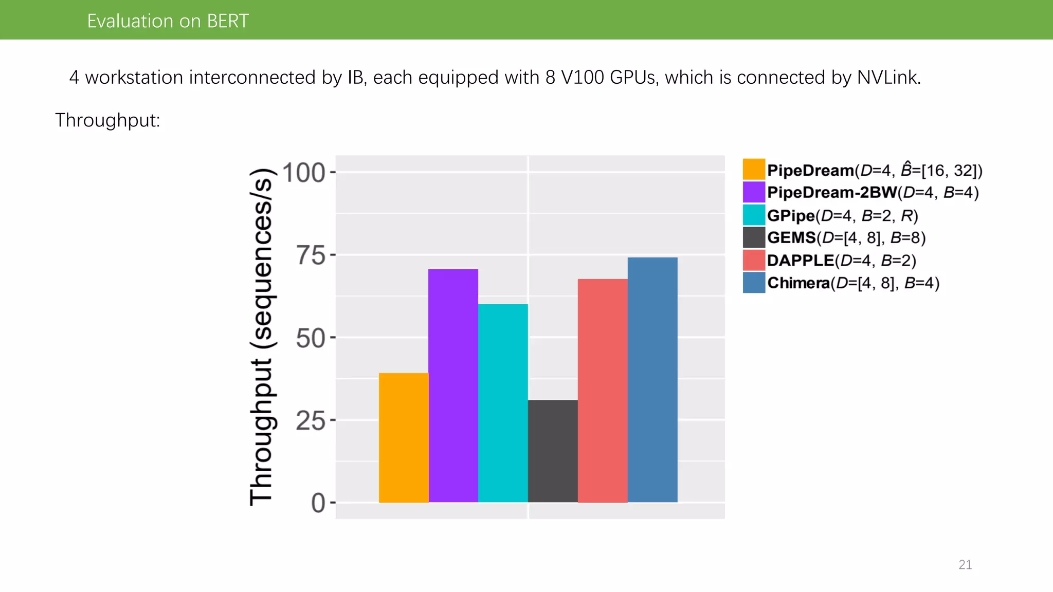
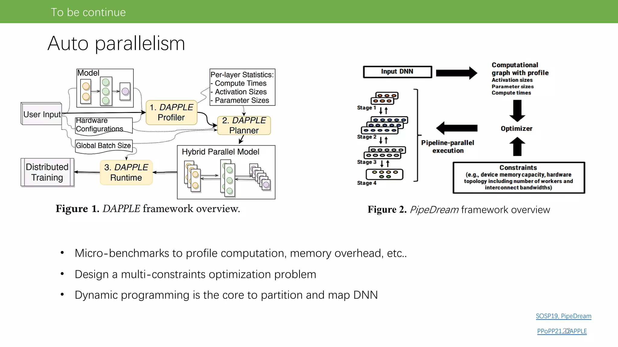
The document discusses pipeline parallel training techniques for large-scale neural networks, highlighting benefits such as reduced communication overhead and improved training efficiency compared to data parallelism. It details various core techniques like micro-batching, gradient checkpointing, and weight stashing to optimize memory and computation during training. The evaluation focuses on frameworks like Pipedream and outcomes from experiments on BERT, outlining the potential for auto parallelism in future applications.

![Why we need it?
Compared to the most prevalent data
parallel, Pipeline Parallel (PP) can:
1. Train a large model
2. Low communication overhead
(around 90% less)
3. It overlaps computation and
communication
Introduction
x[2]
x[3]
x[1]
But, a naive implementation
incurs:
1. Idle devices
2. Low throughput
3. State staleness
3](https://image.slidesharecdn.com/pipelineparalleltrainingoflarge-scaleneuralnetwork-230116031202-9077e290/75/A-review-of-Pipeline-Parallel-Training-of-Large-scale-Neural-Network-pdf-3-2048.jpg)
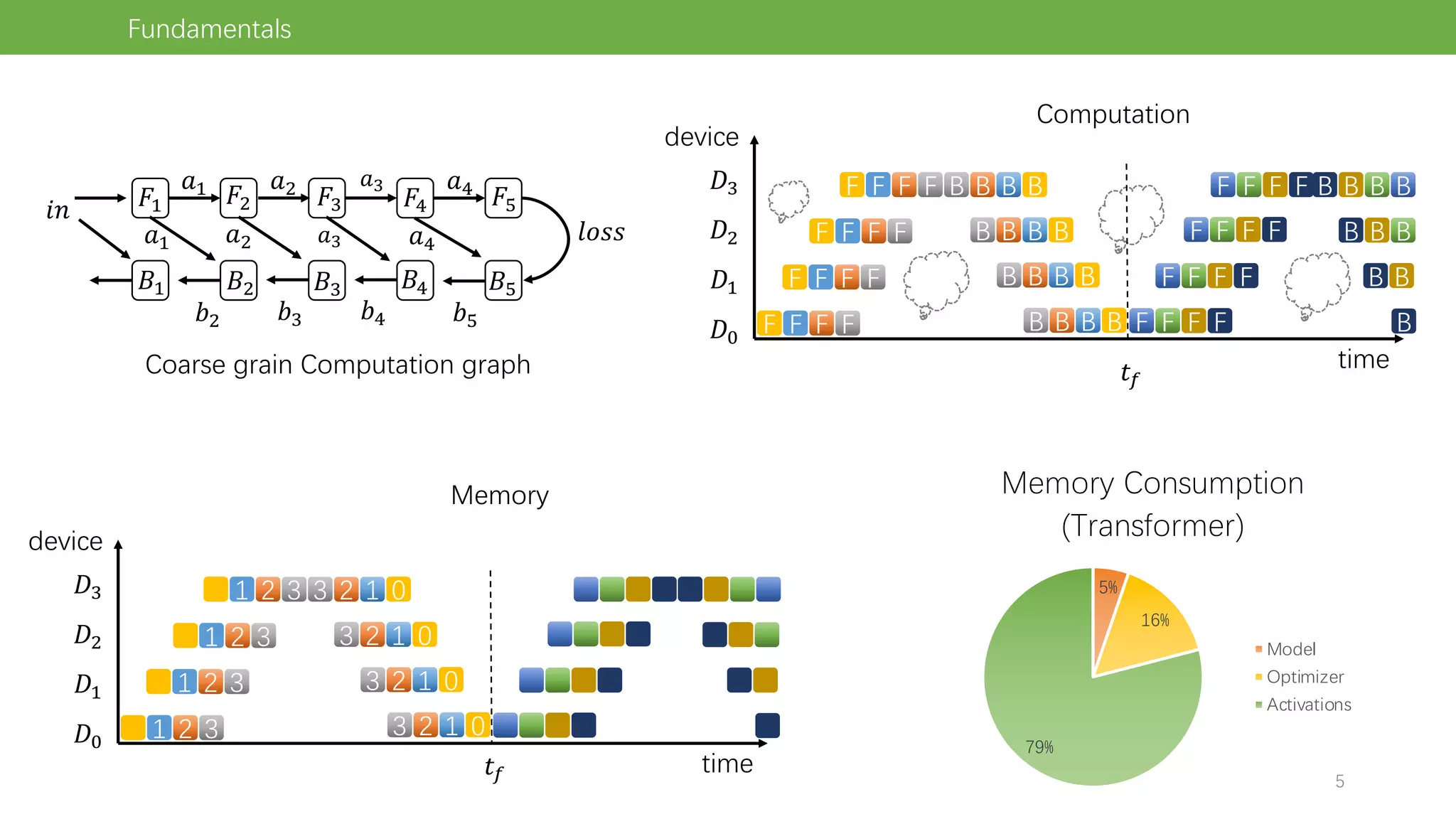
![Fundamentals
x[2]
x[3]
x[1]
!" !# !$ !% !&
Partition the NN into several
stages (continuous sequence
of layers)
All devices are running on
different task and data stream
'" '# '$ '%
Assign stages into a device
time
device
'"
'#
'$
'%
F F F F
F F F F
F F F F
F F F F B B B B
B B B B
B B B B
B B B B F F F F
F F F F
F F F F
F F F F B B B B
B B B
B B
B
4](https://image.slidesharecdn.com/pipelineparalleltrainingoflarge-scaleneuralnetwork-230116031202-9077e290/75/A-review-of-Pipeline-Parallel-Training-of-Large-scale-Neural-Network-pdf-4-2048.jpg)