A credit risk prediction pipeline that utilizes deep learning models for tabular data can outperform state-of-the-art tree-based models like XGBoost, Random Forest, and CatBoost. This pipeline includes: • Tabular data imputation • Tabular data generation • Tabular data risk classification prediction

1. A New State-of-the-Art Credit Risk
Modelling Pipeline with Deep Learning
Tabular Data Models
By Sione. Palu.
Contents
1. Importance of Credit Risk Modelling
2. Challenges in Credit Risk Modelling
3. Widely Adopted Credit Risk Models in Current Practice
a) Logistic Regression Method
b) Ensemble Methods (Random Forest & XGBoost)
c) Deep Learning Methods
4. Missing Data
5. Imputation with Diffusion Models
6. Limitations of Current Methods to Address Imbalanced Data
7. Addressing Imbalanced Datasets with Deep Learning–Based
Tabular Data Generation
8. A New State-of-the-Art Credit Risk Modelling Pipeline
9. Why Choose Deep Learning-Based Tabular Data Classification
Models?
10. Recap and Final Thoughts
11. References

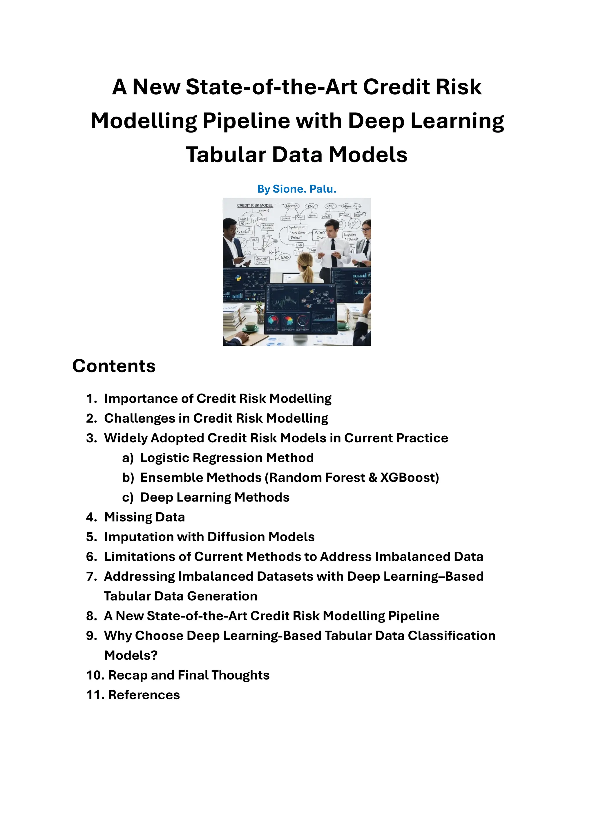
2. 1. Credit Risk Modelling
Credit risk modelling is a statistical process used by financial institutions to assess the
likelihood that a borrower will default on a loan. These models analyse historical and
real-time data to quantify risk, which informs critical business decisions. Without them,
a financial institution would be at a significant disadvantage, leading to poor lending
decisions and potential insolvency.
a) It helps lenders predict the Probability of Default (PD), the Loss Given Default
(LGD), and the Exposure at Default (EAD). By quantifying these risks, institutions
can set appropriate interest rates and lending terms or deny a loan application to
avoid losses.
b) It enables risk-based pricing by financial institutions, where borrowers with lower
risk are offered more favourable rates. This not only attracts high-quality
customers but also ensures that higher-risk loans are priced to compensate for
the greater potential for loss, which protects the lender's profitability.
c) Regulatory Compliance which requires banks to use robust internal models to
calculate and hold sufficient capital reserves against potential losses, ensuring
the stability of the financial system.
2. Challenges in Credit Risk Modelling
The following are some challenges in using ML (machine learning) for credit risk
prediction, as highlighted in Ref [1]:
a) Low Explainability: Many ML models, such as neural networks and boosted
algorithms, operate as black boxes, which makes it difficult to interpret their
predictions. This lack of interpretability hinders their adoption in financial
institutions, where transparency is crucial for regulatory compliance and
decision-making.
b) Data Imbalance and Overfitting: Credit datasets are often imbalanced (e.g., far
more good payers than defaulters), leading to biased models and overfitting. This
reduces performance, especially in real-world scenarios.
c) Data Inconsistency: Datasets may not accurately reflect real-world conditions
due to biases, errors in recording, or missing values.
d) Uncertainty in Dynamic Environments: External factors (e.g., economic
changes like the 2008 crisis or COVID-19) increase uncertainty, making models
less robust. This necessitates the development of adaptable models that
incorporate macroeconomic variables and can handle non-linear relationships.

3. e) Unstructured Data: While unstructured data (e.g., social media posts, news
articles) can provide valuable insights, it is challenging to process and integrate
into traditional models. This is addressed in [2], where user online behavioural
data (e.g., registration, login, click, and authentication behaviours) are utilized.
f) Non-Stationarity: Economic conditions and borrower behaviour change over
time. Models must be continuously monitored and re-calibrated to remain
relevant and accurate, which is a major ongoing challenge.
3. Widely Adopted Credit Risk Models in Current
Practice
While traditional statistical methods remain a cornerstone, the industry is increasingly
adopting more sophisticated machine learning techniques. A few of these are listed
below, but the list is not limited to them:
a) Logistic Regression (LR):
• LR Pros:
➢ This is a classic and highly interpretable model that remains the most
widely adopted for retail credit scoring. Its simplicity and ability to
provide a clear explanation for each variable's impact make it a
favourite of most analysts.
• LR Cons:
➢ Despite these strengths, an LR model often struggles to capture non-
linear relationships and complex interactions between features. This
limitation can negatively impact its predictive power, especially when
the underlying data is not linearly separable. It can also perform poorly
with high-dimensional data, requiring significant manual feature
engineering to be effective.
b) Ensemble (Ens) Methods - Random Forest & XGBoost:
• Ens Pros:
I. Random Forest (RF) and XGBoost models are generally more
accurate than single models like Logistic Regression (LR) and
Decision Trees (DT) because they combine multiple "weak learners"
(decision trees) to boost performance. This ensemble approach
makes them more robust and less prone to overfitting.
II. These models excel at capturing non-linear relationships and
complex feature interactions, making them well-suited for high-
dimensional and complex datasets, like user behavioural data.

4. Additionally, they can handle missing values and outliers to a
certain extent. Both models provide feature importance rankings,
which helps identify the most influential variables. The XGBoost has
built-in mechanisms to handle imbalanced datasets effectively.
• Ens Cons
I. While ensemble methods are powerful, they have drawbacks.
Reduced Interpretability: Unlike simpler models like LR, ensemble
methods are "black boxes". Their complex nature, which involves
combining numerous trees, makes it difficult to understand how they
arrive at a prediction. This lack of transparency can be a major
challenge in regulated industries.
II. They are computationally intensive. They require more time and
resources to train and tune, especially with large datasets. Achieving
optimal performance with these models requires careful
hyperparameter tuning, a process that can be both time-consuming
and complex.
c) Deep Learning (DL) Methods - RNN, LSTM, CNN, Gen-AI:
• DL Pros:
I. Handling unstructured and sequential data is a major area where
deep learning shines. Traditional models like LR and ensemble
methods (Random Forest, XGBoost) are built for structured, tabular
data. However, modern credit risk analysis often involves
unstructured data, such as text from loan application notes, news
articles, or customer communication, as highlighted in Ref [4].
Additionally, sequential data like a borrower's transaction history or
payment patterns over time is best captured by RNNs and LSTMs,
which can learn from the temporal dependencies.
II. Deep learning models, particularly CNNs, can automatically extract
and learn meaningful features from raw data, reducing the need for
extensive manual feature engineering. This capability is crucial
when dealing with high-dimensional or alternative data sources that
might not have a clear, pre-defined structure.
III. By modelling highly non-linear relationships and complex
interactions that are often too intricate for other models, deep
learning can achieve higher predictive accuracy, especially on large
and complex datasets. This leads to more precise risk assessments.
• DL Cons:
I. Deep learning models are often considered "black boxes." Their
complex, multi-layered structure makes it difficult to understand

5. exactly how they arrive at a decision. This lack of transparency is a
significant drawback in the highly regulated financial industry, where
banks must be able to explain the reasons for a loan denial to meet
regulatory requirements (e.g., Fair Credit Reporting Act).
II. Training deep learning models requires a large amount of data to
perform well. They are also computationally intensive, demanding
powerful hardware (like GPUs) and more time for training and tuning
compared to simpler models.
III. While robust, deep learning models with a high number of
parameters are susceptible to overfitting, where they learn the noise
in the training data rather than the underlying pattern. This can lead
to poor performance on new, unseen data if not managed with
proper regularization techniques.
4. Missing Data
Missing data is a common issue that can cause problems for banks, especially in credit
risk portfolios that have a low number of defaults. The problem is made worse when the
missing data belongs to non-worthy applicants who have defaulted. Research, such as
that in Ref [6], has shown that the elimination strategy (i.e., removing records with
missing data) consistently performed the worst across different measures in terms of
credit risk prediction accuracy.
To address the missing data problem, the solution is to impute the missing values. The
authors found that simple mean (for numerical features) and mode (for categorical
features) imputation can work well.
The popular MICE imputation method, which uses a chain of linear regression models
to estimate missing values, has two major limitations, which is highlighted in Ref [7].
First, its regression models can be ineffective if a feature's missing values are
independent of other features. Second, it struggles to capture the non-linear
relationships that are common in real-world data.
Unfortunately, there is no single best imputation method for all datasets or missing
value types; it is highly dependent on the situation. For high dimensional large-scale
datasets, deep learning imputation models are often more appropriate, as they can
address the nonlinearity and scalability challenges of feature interactions.
Some deep learning methods can learn from data with missing values by jointly
imputing and classifying, but this process adds computational cost and can bias
results. An alternative is a deep learning framework that learns directly from observed
values, avoiding the need for synthetic data. Similarly, decision tree-based models like

6. Random Forest and XGBoost can handle missing values directly, though they may be
overfit in high-dimensional feature spaces without incremental learning.
5. Imputation with Diffusion Models
The most significant recent development in deep learning-based tabular data
imputation is the use of Diffusion Models. These models, which have been highly
successful in image and audio generation, have been adapted to handle the unique
challenges of tabular data, including mixed data types and out-of-sample imputation.
Some of the recently published diffusion models are listed below, but the list is not
exhaustive. They use embeddings or a unified encoding scheme to represent mixed-
variate (ie, both numerical and categorical data) and can handle out-of-sample
imputation (i.e., samples not seen in the training set).:
• DiffPuter (2024) – Ref [8]: This model is specifically designed for missing data
imputation in tabular data. It combines a tailored diffusion model with the
Expectation-Maximization (EM) algorithm. It handles both continuous and
categorical variables and has been shown to outperform many existing
imputation methods. DiffPuter is a strong candidate for out-of-sample
imputation as it iteratively fills in missing values by learning the joint distribution
of observed and unobserved data.
• MTabGen / TabGenDDPM (2024) – Ref [9]: This paper proposes a diffusion
model that introduces an encoder-decoder transformer and a dynamic
masking mechanism to handle both imputation and synthetic data generation
within a single framework. This unified approach makes it highly effective for out-
of-sample imputation because the model is trained to condition on existing data
while generating new values, including those for new, completely unobserved
samples. It can handle various feature types and has demonstrated superior
performance on datasets with a large number of features.
• MissDDIM (2025) – Ref [10]: The MissDDIM model addresses the limitations of
stochastic diffusion models, which can suffer from high inference latency and
variable outputs. It offers faster and more stable imputation results, making it
more practical for real-world applications where consistent outputs for new data
are crucial.
6. Limitations of Current Methods to Address
Imbalanced Data
a) Data Class Imbalance

7. I. Definition: Occurs when the target labels (classes) in a classification
task are not represented equally.
II. Example: In a fraud detection dataset, only 1% of transactions are
fraudulent, while 99% are normal.
III. Impact:
➢ Models become biased toward the majority class.
➢ Accuracy may look high (predicting “non-fraud” most of the time), but
performance on the minority class is poor.
b) Group Imbalance
I. Definition: Occurs when subpopulations (groups) within the data are
unequally represented, even if the target classes are balanced. These
groups may correspond to sensitive attributes (e.g., gender, race, age) or
other data partitions (e.g., hospitals, regions, devices).
II. Example: Suppose you have a medical dataset where “disease = yes” and
“disease = no” are equally balanced. However, 90% of the patients are
from Hospital A and only 10% from Hospital B.
III. Impact:
➢ Models may perform well overall but poorly on underrepresented groups.
➢ Leads to fairness issues and reduced generalization.
The key differences between the two types of imbalances are:
- Class (or target) imbalance is about how many examples of each label you have.
- Group imbalance is about which subpopulations are represented in the data,
regardless of class balance.
The class (or target) imbalanced datasets used in classification tasks suffer from the
following issues:
• Bias toward majority class: Models often predict the majority class to maximize
accuracy, ignoring the minority class.
• Poor minority detection: Critical cases (e.g., defaults, fraud, rare diseases) are
missed, leading to low recall and unreliable results.
• Misleading metrics: Accuracy looks high, but meaningful measures like
Precision, Recall, or AUC reveal poor performance
The popular SMOTE (Synthetic Minority Over-sampling Technique) and its derivatives,
which addresses class/target imbalanced datasets, generates new samples by
interpolating between existing minority class instances and their k-nearest neighbors.
While this simple approach is effective for certain datasets, it has several limitations
that deep learning models overcome:

8. • Failure to Capture Complex Distributions: SMOTE operates on a simple linear
interpolation, which assumes a convex shape for the minority class. It fails to
capture complex, non-linear relationships or multi-modal distributions that are
common in real-world tabular data. This can lead to the generation of
"unrealistic" synthetic samples.
• No Inter-feature Correlation: SMOTE treats each feature independently during
interpolation, which means it doesn't learn the complex dependencies and
correlations between different columns. For example, if two columns in a
dataset are highly correlated, SMOTE might generate samples that break this
relationship, hurting the performance of a downstream classifier.
• Categorical Data Challenges: SMOTE is primarily designed for continuous
numerical data. While variations like SMOTE-NC and SMOTE-N exist for
categorical data, they often overgeneralize and can create samples that don't
make sense in a real-world context.
7. Addressing Imbalanced Datasets with Deep
Learning–Based Tabular Data Generation
The advantages of using deep learning models, particularly GANs (Generative
Adversarial Networks) and VAEs (Variational Autoencoders), lie in their ability to
overcome the limitations of SMOTE in addressing data imbalance, as highlighted in the
list below:
• Learning Complex Data Distributions: GANs, such as CTGAN (Conditional
Tabular GAN), learn the entire joint probability distribution of the data. The
adversarial training process between the generator and discriminator forces the
model to create synthetic data that is not only similar to the real data but also
captures the complex, non-linear dependencies and multi-modal distributions
across all features.
• Generating Realistic and Diverse Samples: By modelling the entire data
distribution, these deep generative models can create new, diverse samples that
are more realistic than the linearly interpolated samples from SMOTE. This
reduces the risk of generating samples that fall in "unnatural" regions of the
feature space, leading to better classification performance than SMOTE on
datasets with mixed continuous and categorical features.
• Handling Mixed Data Types: Models like CTGAN are specifically designed to
handle a mix of categorical and continuous variables using specialized encoding
techniques, which is a major advantage over traditional SMOTE methods that
work well only with numerical features.

9. While deep learning-based models often require more computational resources and
can be more complex to train, many models in published studies have demonstrated
superior performance in generating high-quality synthetic data for imbalanced tabular
classification tasks.
More information on tabular data generation to address class and group imbalances
can be found in Ref. [11] and Ref. [12].
8. A New State-of-the-Art Credit Risk Modelling
Pipeline
The workflow shown below depicts a new state-of-the-art credit risk modelling
approach using deep learning-based tabular models:
The workflow overview is highlighted below:
➢ The data is first pre-processed to correct malformed entries (e.g., string entries
in numerical fields or values that appear wrongly scaled) and to flag missing
entries with NaN, preparing them for encoding in the imputation step below.

10. ➢ The pre-processed dataset is then imputed using a deep learning-based tabular
data completion method. The trained completion model is saved for later use.
➢ The completed/imputed dataset from the previous step is then fed into a deep
learning tabular data generation model to produce additional samples. This
enlarges the dataset while reflecting its original distribution, addressing data
sparsity. It also mitigates class/target and group imbalances by generating new
samples for under-represented classes, targets, and groups.
➢ The enlarged generated dataset is then split into training and testing sets.
➢ A deep learning tabular classification model is trained on the training set and its
performance is evaluated on the testing set. If the performance criteria are met,
the final model is packaged for deployment.
➢ During live deployment, when new samples arrive, they are checked for
completeness. If a sample has missing entries, it is first passed through the
trained imputation model before being fed into the trained credit risk
classification model for risk prediction. If a sample has no missing entries, it is
fed directly into the trained classification model for prediction.
9. Why Choose Deep Learning-Based Tabular Data
Classification Models?
Predicting credit risk with high accuracy is critically important because inaccurate
predictions have significant financial and operational consequences. The goal is to
minimize two types of errors: false negatives and false positives.
High-accuracy prediction is crucial, as highlighted in the following points:
➢ Avoids Financial Loss: A false negative occurs when a model incorrectly
predicts that a high-risk borrower will pay back their loan. If the loan is
approved and the borrower defaults, the lender suffers a direct financial loss. A
high-accuracy model reduces these errors, protecting the lender's capital.
➢ Maximizes Profit and Growth: A false positive occurs when a model
incorrectly flags a low-risk borrower as high-risk, leading to a loan application
being denied. A highly accurate model minimizes these errors, ensuring that
profitable, low-risk lending opportunities are not missed. This is essential for a
financial institution's growth.
➢ Regulatory Compliance and Ethics: In many jurisdictions, regulations like the
Fair Credit Reporting Act (in the U.S.) and GDPR (in the EU) require lenders to
provide clear, fair, and justifiable reasons for credit decisions. Highly accurate
models that are also interpretable help financial institutions comply with these
regulations and avoid legal and reputational risk.

11. The deep learning-based tabular data classification models listed below have shown to
be more accurate in most tests (or on par in some cases) compared to popular tree-
based models such as XGBoost, Random Forest, and CatBoost.
▪ As shown in the study in [13], TabICL surpasses tree-based models like XGBoost
and CatBoost on classification tasks in terms of accuracy and AUC.
▪ TabR outperformed XGBoost on a benchmark test, which is described in [14]
▪ AMFormer demonstrated superior overall performance compared to XGBoost,
scoring the highest in key metrics such as AUC, MCC, and F1 in the study
described in [15]
▪ The research in [16] indicates that while XGBoost is a strong contender in the
benchmark classification test, the TabM model achieved better or competitive
performance, particularly when properly tuned.
▪ The Mambular model, described in [17], is benchmarked classification task
against state-of-the-art models, including other neural networks and tree-based
methods like XGBoost and CatBoost, and its performance was found to be on
par with or better than theirs (in some datasets).
▪ The Beta model described in [18], which is an enhancement of the TabPFN
model, either outperforms or matches state-of-the-art methods like CatBoost
and XGBoost on over 200 benchmark classification datasets.
▪ The TabNet model, described in the study in [19], significantly outperformed
XGBoost in both binary and multi-class classification tasks but only after
extensive hyperparameter tuning.
10. Recap and Final Thoughts
While tree-based models like XGBoost and Random Forest have long been the industry
standard, deep learning models are emerging as a more favourable solution for modern
credit risk prediction. They offer a powerful and flexible approach that can overcome the
limitations of traditional methods, particularly when dealing with the complex, high-
dimensional, and often messy data of today. The superior capabilities are summarized
below:
• Holistic Data Handling: Deep learning pipelines are uniquely equipped to
handle the entire credit risk data ecosystem, from dealing with missing values
using advanced diffusion models to generating high-quality synthetic data to
overcome class and group imbalances. This integrated approach allows for more
robust and reliable modelling than traditional methods.
• Superior Performance on Complex Data: Deep learning models can capture
intricate, non-linear relationships and interactions within the data that tree-
based models often miss. As the preceding sections have shown, models like
TabICL, AMFormer, and TabR have demonstrated superior or competitive

12. performance against established baselines, particularly on larger and more
complex datasets.
• Adaptability to Evolving Data: Deep learning models are highly adaptable and
excel at processing a wide variety of data types, including unstructured and
sequential data like the loan officer notes. This ability to integrate alternative
data sources provides a more comprehensive view of risk and allows for a more
responsive risk assessment.
11. References:
1. “Machine Learning for Credit Risk Prediction: A Systematic Literature Review”,
J.P. Noriega, et al.
2. “A Deep Learning Approach for Credit Scoring Using Feature Embedded
Transformer” by Chongren Wang, et al.
3. A Deep Learning-based Model for P2P Micro-loan Default Risk Prediction, by
Siwei Xia, et al.
4. "Enhancing Credit Scoring with Multimodal Deep Learning: A Hybrid Neural
Network Approach Using Structured and Unstructured Financial Data", by Md
Refat Hossain, et al.
5. “Credit Risk Scoring with TabNet Architecture”, by A.B. Yuksel, et al.
6. "Investigating the missing data effect on credit scoring rule-based models", by S.
M. Sadatrasoul, et al.
7. "Imputation is Not Required: Incremental Feature Attention Learning of Tabular
Data with Missing Values", by M.D. Samad, et al.
8. "DiffPuter: Empowering Diffusion Models for Missing Data Imputation", by
Hengrui Zhang, et al.
9. "Diffusion Models for Tabular Data Imputation and Synthetic Data Generation",
by M. Villaizán-Vallelado, et al.
10. "MissDDIM: Deterministic and Efficient Conditional Diffusion for Tabular Data
Imputation", by Youran Zhou,et al.
11. "Synthetic Tabular Data Generation for Class Imbalance and Fairness: A
Comparative Study", by Arjun Roy, et al.
12. "TabFairGAN: Fair Tabular Data Generation with Generative Adversarial
Networks", by A. Rajabi, et al.
13. "TabICL: A Tabular Foundation Model for In-Context Learning on Large Data", by
Jingang Qu, et al.
14. "TabR: Tabular Deep Learning Meets Nearest Neighbors", by Yury Gorishniy, et al.
15. "Arithmetic Feature Interaction Is Necessary for Deep Tabular Learning", by Yi
Cheng, et al.
16. "TabM: Advancing Tabular Deep Learning With Parameter-Efficient Ensembling",
by Yury Gorishniy, et al.

13. 17. "Mambular: A Sequential Model for Tabular Deep Learning", by Soheila Samiee,
et al.
18. "TabPFN Unleashed: A Scalable and Effective Solution to Tabular Classification
Problems", by Si-Yang Liu, et al.
19. "TabNet: Attentive Interpretable Tabular Learning", by Tomas Pfister, et al.