9-2020.pdf

applied
sciences
Article
Artificial Intelligence Enabled Routing in Software
Defined Networking
Yan-Jing Wu 1,* , Po-Chun Hwang 2, Wen-Shyang Hwang 2 and Ming-Hua Cheng 3
1 Department of Information Technology and Communication, Shih Chien University, Kaohsiung Campus,
Kaohsiung 845, Taiwan
2 Department of Electrical Engineering, National Kaohsiung University of Science and Technology,
Jiangong Campus, Kaohsiung 807, Taiwan; 1103104147@gm.kuas.edu.tw (P.-C.H.);
wshwang@nkust.edu.tw (W.-S.H.)
3 Department of Digital Media Design, Tzu-Hui Institute of Technology, Pingtung 926, Taiwan;
cmha6777@mail.tzuhui.edu.tw
* Correspondence: yanjing@g2.usc.edu.tw
Received: 25 August 2020; Accepted: 17 September 2020; Published: 20 September 2020

Abstract: Software defined networking (SDN) is an emerging networking architecture that separates
the control plane from the data plane and moves network management to a central point, called the
controller. The controller is responsible for preparing the flow tables of each switch in the data plane.
Although dynamic routing can perform rerouting in case of congestion by periodically monitoring
the status of each data flow, problems concerning a suitable monitoring period duration and lack of
learning ability from past experiences to avoid similar but ineffective route decisions remain unsolved.
This paper presents an artificial intelligence enabled routing (AIER) mechanism with congestion
avoidance in SDN, which can not only alleviate the impact of monitoring periods with dynamic
routing, but also provide learning ability and superior route decisions by introducing artificial
intelligence (AI) technology. We evaluate the performance of the proposed AIER mechanism on the
Mininet simulator by installing three additional modules, namely, topology discovery, monitoring
period, and an artificial neural network, in the control plane. The effectiveness and superiority of our
proposed AIER mechanism are demonstrated by performance metrics, including average throughput,
packet loss ratio, and packet delay versus data rate for different monitoring periods in the system.
Keywords: software defined networking; artificial neural network; routing; monitoring period
1. Introduction
1.1. Software-Defined Networking
The revolutionary technology of radio access network (RAN) in each generation is obvious from
the first generation of mobile communications (1G) to the fifth generation of mobile communications
(5G) and beyond, but the revolution is not in core network (CN) technology. Only the 3G era has
experienced a major change from circuit switching to packet switching. Considering that global
operators have invested huge funds in the previous CN technology, the CN technology revolution
at the 3G stage allows the two switching modes to coexist and make the operators freely choose to
adopt circuit or packet switching mode until the 4G era comes, which is officially integrated into
the all-IP (Internet Protocol) packet switching core network system. With the growing demands for
wireless mobile communications in the Internet of things (IoT) society after 2020, 5G is regarded
as a revolutionary technology with great hopes and an innovation in the RAN technology. As to
the CN technology in 5G, it is expected to meet the needs of the rapid development of various
services that include a wide range of data and connections in the future, and to ultimately meet the
Appl. Sci. 2020, 10, 6564; doi:10.3390/app10186564 www.mdpi.com/journal/applsci

Appl. Sci. 2020, 10, 6564 2 of 16
user-centric wireless communications. One of the most important key to networking requirements
is the development of two technologies, software-defined networking (SDN) and network-function
virtualization (NFV) [1]. SDN is a kind of control signaling and user data separation, centralized control
of network functions, and open application interface (API). After the introduction of SDN, the new
challenges are how to reconstruct network functions, how to design new interface protocols, and then
optimize the architecture and end-to-end signaling process based on SDN. Similar to some concepts of
SDN, NFV uses cloud virtualization-based information technologies to transform 4G/5G core network,
using general purpose platform (GPP) to build the basic telecommunications environment. Focusing
on applying artificial intelligence (AI) technology to CN routing, this paper presents an AI-enabled
routing scheme specifically for SDN because the core concepts of both SDN and NFV technologies
are quite similar and the two have high conditions for complementary integration. Based on SDN
architecture, several works have been proposed to successfully overcome the limitations regarding
the de-facto standard simulator, Mininet [2], or the implementation of multi-domain connectivity
services [3–7].
SDN is an emerging networking architecture that consists of three layers [8,9], namely, the application,
control, and data planes (see Figure 1). SDN is programmable through logically centralized management
to simplify complex network tasks, such as route optimization, traffic engineering and so on for
increasingly diversified network deployment. The SDN control plane is required to discover a network
topology of the entire SDN infrastructure mainly for configuring data transmission paths between any
source-to-destination pairs in the data plane. However, discovering a network topology is challenging
due to frequent migration of the virtual machines in the data plane, lack of authentication standards,
and so on. For the purpose, the authors of [10] have presented a comprehensive survey of the topology
discovery and the associated security implications in SDNs. The application programming interface
that resides between the control and application planes is called the northbound interface, where a set of
network services such as quality of service (QoS), intrusion detection, and monitoring functions can be
implemented. Communication interface between the control and data planes is called the southbound
interface, where the OpenFlow protocol [11] is commonly used to exchange control messages with
forwarding devices, referred to as OpenFlow switches. An OpenFlow switch comprises one or more
flow tables, a group table, and an OpenFlow channel for the external controller. OpenFlow switches
handle arriving packets by checking if any flow entries in their flow tables match the new arriving
packets and whether or not to perform forwarding. A flow table consists of a set of flow entries.
Using the OpenFlow protocol, the controller in the control plane can add, update, and delete flow
entries in the flow table(s) of an OpenFlow switch via the OpenFlow channel. Figure 2 shows the
six main components of flow entry, namely, match fields, priority, counters, instructions, timeouts,
and cookies [12]. “Match fields” are used to match the ingress port number and part of the information
contained in the packet header. Flow entries match packets in “priority” order, to the first matching
entry being used in each table. If a matching entry is found, then “instructions” associated with the
specific flow entry are executed. “Counters” are updated simultaneously when packets are matched.
If no match is found, then the forwarding decision will depend on the configuration of the table-miss
flow entry. “Timeouts” indicate the maximum amount of time or idle time before the expiration of the
flow entry. The “cookie” falls under opaque data, which may be used by the controller to filter, modify,
or delete flow statistics, but not to process packets.

Appl. Sci. 2020, 10, 6564 3 of 16
Appl. Sci. 2020, 10, x 3 of 16
Figure 1. Software defined networking (SDN) architecture.
Figure 2. Main components of flow entry.
1.2. Artificial Intelligence Enabled Routing
Notably, in the recent decade, performance has improved in numerous fields with the
application of artificial intelligence (AI) technology [13]. The networking field is no exception. The
well-known Turing test [14] considers machines intelligent if humans cannot distinguish them from
a man when talking to them. In 1980, John Searle classified AI into strong and weak types [15]. A
strong AI has a complex algorithm that can help it act in different situations, whereas the actions of
a weak AI are preprogrammed by a person. In other words, strong AI-enabled machines have the
ability to apply intelligence to any problem rather than only specific problems, whereas weak AI-
enabled machines can only simulate human behavior. As illustrated in Figure 3, machine learning
(ML), which describes a methodology implementing AI, is a growing subfield of AI [16]. Support
vector machines (SVMs) [17], decision trees [18], random forests [19], artificial neural networks
(ANNs) [20], and so on have been presented sequentially as ML technologies. As to deep learning
(DL), it is a family of machine learning methods based on ANNs with representation learning.
Learning can be supervised, semi-supervised, or unsupervised. The “deep“ in DL comes from that
two or more hidden layers are used in the network. In other words, an unbounded number of layers
of bounded size constitute an ANN model, which allows practical application and optimized
implementation while retaining theoretical universality under mild conditions [21].
Appl. Sci. 2020, 10, x 3 of 16
Notably, in the recent decade, performance has improved in numerous fields with the
application of artificial intelligence (AI) technology [13]. The networking field is no exception. The
well-known Turing test [14] considers machines intelligent if humans cannot distinguish them from
a man when talking to them. In 1980, John Searle classified AI into strong and weak types [15]. A
strong AI has a complex algorithm that can help it act in different situations, whereas the actions of
a weak AI are preprogrammed by a person. In other words, strong AI-enabled machines have the
ability to apply intelligence to any problem rather than only specific problems, whereas weak AI-
enabled machines can only simulate human behavior. As illustrated in Figure 3, machine learning
(ML), which describes a methodology implementing AI, is a growing subfield of AI [16]. Support
vector machines (SVMs) [17], decision trees [18], random forests [19], artificial neural networks
(ANNs) [20], and so on have been presented sequentially as ML technologies. As to deep learning
(DL), it is a family of machine learning methods based on ANNs with representation learning.
Learning can be supervised, semi-supervised, or unsupervised. The “deep“ in DL comes from that
two or more hidden layers are used in the network. In other words, an unbounded number of layers
of bounded size constitute an ANN model, which allows practical application and optimized
implementation while retaining theoretical universality under mild conditions [21].
Notably, in the recent decade, performance has improved in numerous fields with the application
of artificial intelligence (AI) technology [13]. The networking field is no exception. The well-known
Turing test [14] considers machines intelligent if humans cannot distinguish them from a man when
talking to them. In 1980, John Searle classified AI into strong and weak types [15]. A strong AI
has a complex algorithm that can help it act in different situations, whereas the actions of a weak
AI are preprogrammed by a person. In other words, strong AI-enabled machines have the ability
to apply intelligence to any problem rather than only specific problems, whereas weak AI-enabled
machines can only simulate human behavior. As illustrated in Figure 3, machine learning (ML),
which describes a methodology implementing AI, is a growing subfield of AI [16]. Support vector
machines (SVMs) [17], decision trees [18], random forests [19], artificial neural networks (ANNs) [20],
and so on have been presented sequentially as ML technologies. As to deep learning (DL), it is a
family of machine learning methods based on ANNs with representation learning. Learning can be
supervised, semi-supervised, or unsupervised. The “deep“ in DL comes from that two or more hidden
layers are used in the network. In other words, an unbounded number of layers of bounded size
constitute an ANN model, which allows practical application and optimized implementation while
retaining theoretical universality under mild conditions [21].

Appl. Sci. 2020, 10, 6564 4 of 16
Appl. Sci. 2020, 10, x 4 of 16
Figure 3. Evolution of artificial intelligence (AI).
An ANN mainly simulates human brain nerves using mathematical models. In contrast to
human brain nerves (see Figure 4a), inputs x1, x2, and x3 of an ANN (see Figure 4b) simulate human
brain nerve dendrites; weights w1, w2, and w3 of an ANN simulate axons; and the deviation value of
an ANN (denoted by b) simulates a synapse, which is a critical action value of a neuron. Equation (1)
represents the operation mode of one neuron, where y denotes the output. To handle complex
nonlinear problems, Equation (1) is further substituted with an activation function to form a
differentiable nonlinear function, as expressed by Equation (2). Through the backpropagation
algorithm (BPA) [22], the optimization gradient descent method can be used to continuously
iteratively compute and update the weights in the ANN model such that the model output can
approach the expected value, that is, the corresponding label data (designated as yi’), until the error
function (see Equation (3)) converges.
1 1 2 2 3 3
y x w x w x w
   (1)
1 1 2 2 3 3
( )
y Activation function x w x w x w
   (2)
2
0
( ')
i i
i
Loss function y y

 
 (3)
where i indicates the i-th record of training data.
(a) (b)
Figure 4. (a) A neuron of Human brain nerves; (b) ANN model for simulating a neuron.
Since the layers of an ANN in DL are allowed to be heterogeneous and to deviate widely from
biologically informed connectionist models for the sake of efficiency, trainability, and
An ANN mainly simulates human brain nerves using mathematical models. In contrast to human
brain nerves (see Figure 4a), inputs x1, x2, and x3 of an ANN (see Figure 4b) simulate human brain
nerve dendrites; weights w1, w2, and w3 of an ANN simulate axons; and the deviation value of an
ANN (denoted by b) simulates a synapse, which is a critical action value of a neuron. Equation (1)
represents the operation mode of one neuron, where y denotes the output. To handle complex nonlinear
problems, Equation (1) is further substituted with an activation function to form a differentiable
nonlinear function, as expressed by Equation (2). Through the backpropagation algorithm (BPA) [22],
the optimization gradient descent method can be used to continuously iteratively compute and update
the weights in the ANN model such that the model output can approach the expected value, that is,
the corresponding label data (designated as yi’), until the error function (see Equation (3)) converges.
y = x1w1 + x2w2 + x3w3 (1)
y = Activation function(x1w1 + x2w2 + x3w3) (2)
Loss function =
X
i=0
(yi − yi
0
)2
(3)
Appl. Sci. 2020, 10, x 4 of 16
An ANN mainly simulates human brain nerves using mathematical models. In contrast to
human brain nerves (see Figure 4a), inputs x1, x2, and x3 of an ANN (see Figure 4b) simulate human
brain nerve dendrites; weights w1, w2, and w3 of an ANN simulate axons; and the deviation value of
an ANN (denoted by b) simulates a synapse, which is a critical action value of a neuron. Equation (1)
represents the operation mode of one neuron, where y denotes the output. To handle complex
nonlinear problems, Equation (1) is further substituted with an activation function to form a
differentiable nonlinear function, as expressed by Equation (2). Through the backpropagation
algorithm (BPA) [22], the optimization gradient descent method can be used to continuously
iteratively compute and update the weights in the ANN model such that the model output can
approach the expected value, that is, the corresponding label data (designated as yi’), until the error
function (see Equation (3)) converges.
1 1 2 2 3 3
y x w x w x w
   (1)
1 1 2 2 3 3
( )
y Activation function x w x w x w
   (2)
2
0
( ')
i i
i
Loss function y y

 
 (3)
(a) (b)
biologically informed connectionist models for the sake of efficiency, trainability, and
biologically informed connectionist models for the sake of efficiency, trainability, and understandability,
this paper presents an AI-enabled routing (AIER) mechanism with congestion avoidance by introducing

Appl. Sci. 2020, 10, 6564 5 of 16
an ANN model in the control plane of SDN for intelligent path selection. The successful application of
ANNs for the AIER not only can alleviate the impact of monitoring periods with dynamic routing
but also can provide the learning ability to make superior routing decisions from past experiences.
It is also demonstrated that the proposed AIER outperforms the SDN routing schemes with no AI
application via simulations. The significant improvement in the average throughput, packet loss ratio,
and packet delay versus data rate for different monitoring periods in the system can be observed.
The remainder of this paper is organized as follows. Section 2 discusses works related to
our proposed AIER mechanism in SDN, and the proposed AIER scheme is elaborated in Section 3.
Simulation results and performance evaluation discussions are presented in Section 4. Finally,
concluding remarks are given in Section 5.
2. Related Works
Packets passing through a route from source to destination nodes encounter various delay
types [23], such as processing, queuing, transmission, and propagation delays. Packet delay causes
packet loss and throughput degradation during transmission. SDN routing schemes are generally
classified into two types, namely, static and dynamic. With static routing, the well-known Dijkstra
algorithm [24] considered only edge weights in the associated network topology to find the shortest
path for data transmission. The authors of [25] extended the Dijkstra algorithm by taking into account
node weights to select a route that is better than the shortest path in terms of distance. Besides,
the authors of [26] used depth-first search to find multiple paths from source-to-destination nodes in a
hierarchical network topology then determined the best path using worst-fit searching. However, a
selected route will not change with static routing unless a link breakup is detected.
To avoid excessive single-link burden and packet loss caused by static routing due to diversified
network conditions, such as burst traffic, link breakups, and device crashes, dynamic routing schemes
have been proposed. Lan et al. [27] proposed a dynamic routing scheme with load-balanced path
configuration. Song et al. [28] calculated each path utilization at the controller with link utilizations
being received periodically from the data plane, and then changed the forwarding path, if necessary.
The authors of [29] presented an effective dynamic routing mechanism with which the controller is
aware of each link status and connected port number between any two switches in the data plane
through the link layer discovery protocol [30]. The connected port number was then used to configure
the corresponding flow entry on each switch according to a route selection algorithm. To reduce packet
loss during path reconfiguration, rerouting was triggered when the link utilization of the current path
exceeds 80%.
Although dynamic routing can perform rerouting under certain pre-defined conditions by
periodically monitoring the status of each data flow, problems concerning a suitable monitoring period
duration and the lack of learning ability from past experiences to avoid similar but ineffective path
decisions remain unsolved. The authors of [31] emphasized that the monitoring period duration
has a significant impact on network performance. A monitoring period that is too short may cause
excessive communication burden on the southbound interface. By contrast, a monitoring period
that is too long may cause the control plane to obtain outdated information from the data plane.
Therefore, the monitoring period duration is crucial for dynamic routing. Besides, the configuration
of an alternative path in the data plane is time consuming. That is, data transmission through the
original path may result in packet loss due to link congestion before the completion of the alternative
path configuration. Furthermore, the system traffic load usually varies with time. Given Figure 5 as
an example, the selected path can afford data transmission from 10 to 50 s in the case of light load.
However, the selected path may cause congestion in the case of heavy load at about 60 s. Although the
control plane can find an alternative path to alleviate congestion, the alternative path will be rerouted
to the previously-selected path due to the shortest path selection from 70 to 110 s. At approximately
120 s, link congestion may occur again in the case of heavy load. Meanwhile, an alternative path same

Appl. Sci. 2020, 10, 6564 6 of 16
as the one decided at 60 s is selected again. In other words, dynamic routing schemes are blind to past
experiences and thus lack learning abilities.
Appl. Sci. 2020, 10, x 6 of 16
alternative path same as the one decided at 60 s is selected again. In other words, dynamic routing
schemes are blind to past experiences and thus lack learning abilities.
Figure 5. Example of the system load vs. time.
In recent years, several routing mechanisms [32–38] combined with AI technology have been
proposed to enhance learning ability from past experiences and smart route-decision capability,
thereby improving overall network performance. First of all, the works in [33–35] introduced AI
technology to routing protocols for wireless sensor networks in order to improve the energy
consumption of each node. On the other hand, the authors of [36] implemented an intelligent routing
protocol in a particular, simple SDN topology. Their proposed intelligent routing protocol was based
on the reinforcement learning process to choose the best data transmission paths according to the
best criteria in terms of weights periodically rewarded by each node on the current path. However, a
formula associated with the cost function was not specifically defined and the impact of rewarding
periods was not considered. Pasca et. al. [37] proposed an application-aware multipath flow routing
framework (AMPS) by enabling the controller of SDN to prioritize each flow using machine learning
techniques and to assign one or more paths based on its classified priority even if the flow are
between the same pair of nodes. The main contribution of AMPS controller in comparison to SDN
with traditional routing is its ensuring high availability of an unloaded path for high priority flows
even in a heavily loaded network. Fu et. al. [38] presented a routing strategy based on deep Q-
learning (DQL) to generate optimal routing paths autonomously for SDN-based data center
networks. However, they aimed to provide different quality of service guarantees for mice-flows and
elephant-flows, designated in a data center network.
The aforementioned works have obtained considerable improvement on network performance
by introducing AI technology. To avoid network congestion that may cause serious packet delay,
packet loss and throughput degradation, this paper proposes an AIER mechanism by introducing an
ANN model to the controller of SDN that uses flow load and link load as the feature data, and
queuing size of an OpenFlow switch as label data. The proposed AIER mechanism consists of three
stages: (1) collection of a set of adequate data for model training, (2) establishment of an ANN model
in the control plane using the training data, and (3) application of the ANN model for path selection.
3. Proposed AIER Mechanism
3.1. System Architecture
The SDN architecture we consider is illustrated in Figure 6. The routing module in the
application plane is used to find the route between any source-to-destination pairs at the beginning.
In the control plane, the well-established Ryu controller [39] is adopted. There are three modules in
the controller, topology discovery, period monitor, and an ANN model, which are used to explore
Figure 5. Example of the system load vs. time.
In recent years, several routing mechanisms [32–38] combined with AI technology have been
proposed to enhance learning ability from past experiences and smart route-decision capability,
thereby improving overall network performance. First of all, the works in [33–35] introduced
AI technology to routing protocols for wireless sensor networks in order to improve the energy
consumption of each node. On the other hand, the authors of [36] implemented an intelligent routing
protocol in a particular, simple SDN topology. Their proposed intelligent routing protocol was based
on the reinforcement learning process to choose the best data transmission paths according to the
best criteria in terms of weights periodically rewarded by each node on the current path. However, a
formula associated with the cost function was not specifically defined and the impact of rewarding
periods was not considered. Pasca et al. [37] proposed an application-aware multipath flow routing
framework (AMPS) by enabling the controller of SDN to prioritize each flow using machine learning
techniques and to assign one or more paths based on its classified priority even if the flow are between
the same pair of nodes. The main contribution of AMPS controller in comparison to SDN with
traditional routing is its ensuring high availability of an unloaded path for high priority flows even in
a heavily loaded network. Fu et al. [38] presented a routing strategy based on deep Q-learning (DQL)
to generate optimal routing paths autonomously for SDN-based data center networks. However, they
aimed to provide different quality of service guarantees for mice-flows and elephant-flows, designated
in a data center network.
The aforementioned works have obtained considerable improvement on network performance
by introducing AI technology. To avoid network congestion that may cause serious packet delay,
packet loss and throughput degradation, this paper proposes an AIER mechanism by introducing an
ANN model to the controller of SDN that uses flow load and link load as the feature data, and queuing
size of an OpenFlow switch as label data. The proposed AIER mechanism consists of three stages:
(1) collection of a set of adequate data for model training, (2) establishment of an ANN model in the
control plane using the training data, and (3) application of the ANN model for path selection.
3. Proposed AIER Mechanism
3.1. System Architecture
The SDN architecture we consider is illustrated in Figure 6. The routing module in the application
plane is used to find the route between any source-to-destination pairs at the beginning. In the control
plane, the well-established Ryu controller [39] is adopted. There are three modules in the controller,

Appl. Sci. 2020, 10, 6564 7 of 16
topology discovery, period monitor, and an ANN model, which are used to explore the link states of the
OpenFlow switches, periodically receive the exchange information from the data plane, and implement
the proposed AIER mechanism to select an intelligent path with congestion avoidance, respectively.
The data plane consists of n source nodes (denoted as S1, S2, . . . , Sn), m destination nodes (denoted as
D1, D2, . . . , Dm), and a number of OpenFlow switches. Therefore, we assume that a maximum of m·n
(denoted as d) data flows are generated and a total of R paths between any source-to-destination pairs
are available.
Appl. Sci. 2020, 10, x 7 of 16
the link states of the OpenFlow switches, periodically receive the exchange information from the data
plane, and implement the proposed AIER mechanism to select an intelligent path with congestion
avoidance, respectively. The data plane consists of n source nodes (denoted as S1, S2, …, Sn), m
destination nodes (denoted as D1, D2, …, Dm), and a number of OpenFlow switches. Therefore, we
assume that a maximum of m∙n (denoted as d) data flows are generated and a total of R paths between
any source-to-destination pairs are available.
Figure 6. Software-defined networking (SDN) architecture with the proposed artificial intelligence
enabled routing (AIER).
3.2. AIER Mechanism
Assuming that there are no link fabrication attacks and no migration of OpenFlow switches [40],
the proposed AIER mechanism adds an ANN model in the SDN controller. First, the AIER
mechanism collects a set of training data in which each record consists of feature data and label data.
Next, the training data are used to train the ANN model, iteratively. The routing algorithm obtains
learning abilities after model training has been completed. Thus, the AIER mechanism not only can
predict the corresponding output based on the new data but also can select a suitable path to avoid
congestion. Figure 7 shows the pseudo code of the proposed AIER mechanism, which includes the
following three stages.
3.2.1. Collection of Training Data
Prior to training the ANN model, an adequately large set of training data is collected in which
each record contains a congestion flag, the generation rates of all data flows, and every allocated path
from a source to a destination. As illustrated in Figure 8, let n = 3, m = 1, and R = 3 as an example.
Table 1 shows the training data set, including every field of each record and several data samples.
Field “C” can be 1 or 0 depending on whether there exists one or more OpenFlow switch whose
queuing length is larger than 80% along the allocated path. If yes, then C is 1; otherwise, C is 0. The d
fields immediately following from Field “C” represent the data generation rates of d data flows. The
last d fields indicate the allocated path number (belonging to {0, 1, 2}) for each data flow.
Figure 6. Software-defined networking (SDN) architecture with the proposed artificial intelligence
enabled routing (AIER).
3.2. AIER Mechanism
Assuming that there are no link fabrication attacks and no migration of OpenFlow switches [40],
the proposed AIER mechanism adds an ANN model in the SDN controller. First, the AIER mechanism
collects a set of training data in which each record consists of feature data and label data. Next,
the training data are used to train the ANN model, iteratively. The routing algorithm obtains learning
abilities after model training has been completed. Thus, the AIER mechanism not only can predict the
corresponding output based on the new data but also can select a suitable path to avoid congestion.
Figure 7 shows the pseudo code of the proposed AIER mechanism, which includes the following
three stages.
3.2.1. Collection of Training Data
Prior to training the ANN model, an adequately large set of training data is collected in which each
record contains a congestion flag, the generation rates of all data flows, and every allocated path from
a source to a destination. As illustrated in Figure 8, let n = 3, m = 1, and R = 3 as an example. Table 1
shows the training data set, including every field of each record and several data samples. Field “C”
can be 1 or 0 depending on whether there exists one or more OpenFlow switch whose queuing length is
larger than 80% along the allocated path. If yes, then C is 1; otherwise, C is 0. The d fields immediately
following from Field “C” represent the data generation rates of d data flows. The last d fields indicate
the allocated path number (belonging to {0, 1, 2}) for each data flow.

Appl. Sci. 2020, 10, 6564 8 of 16
Appl. Sci. 2020, 10, x 8 of 16
Input :
Number of source nodes: n
Number of destination nodes: m
Number of available paths: R
ANN model, which is obtained by training data and validated by test data
Loads for all data flows: L= L1, L2, …, Ld // d = mn
All available path configurations: P1, P2, …, PS, // S = Rd
, |Pk| = d
Output :
Minimum congestion probability (Cmin) among all path configurations
1. set C= [ ]
2. while L1, L2, …., Ld has variation do
3. for each Pk do
4. ANN model input (L, Pk)
5. Ck = ANN model output
6. Append(C, Ck)
7. end for
8. Cu = congestion probability of the current path configuration
9. Cmin = min{C}
10. if Cmin Cu (Cu − Cmin) Th
11. Conduct path reconfiguration to Pk with Cmin
12. end if
13. if queuing length of any switch in the current path configuration 80%
14. Trigger path reconfiguration
15. end if
Figure 7. Pseudo code of the artificial intelligence enabled routing (AIER) mechanism.
Figure 8. Example of the data plane in SDN.
Table 1. Fields in the training data set.
C
Congestion
Flag
S1-D1
Data
Flow
S2-D1
Data
Flow
S3-D1
Data
Flow
S1-D1
Allocated
Path number
S2-D1
Allocated
Path number
S3-D1
Allocated
Path number
0 57M 55M 70M 0 1 2
1 65M 63M 30M 0 0 1
0 65M 50M 65M 0 2 1
3.2.2 ANN Model Training
After the first stage is complete, we use the BPA algorithm [22] to train the ANN model. The
training data require preprocessing before the model is trained. Separating the label data and feature
data in the training data set, we consider Field “C” as the label data (in red) and the other fields as
the feature data (in blue), as shown in Table 2. The feature data of each record are the inputs of a
Appl. Sci. 2020, 10, x 8 of 16
Input :
Number of source nodes: n
Number of destination nodes: m
Number of available paths: R
ANN model, which is obtained by training data and validated by test data
Loads for all data flows: L= L1, L2, …, Ld // d = mn
All available path configurations: P1, P2, …, PS, // S = Rd
, |Pk| = d
Output :
Minimum congestion probability (Cmin) among all path configurations
1. set C= [ ]
2. while L1, L2, …., Ld has variation do
3. for each Pk do
4. ANN model input (L, Pk)
5. Ck = ANN model output
6. Append(C, Ck)
7. end for
8. Cu = congestion probability of the current path configuration
9. Cmin = min{C}
10. if Cmin Cu (Cu − Cmin) Th
11. Conduct path reconfiguration to Pk with Cmin
12. end if
13. if queuing length of any switch in the current path configuration 80%
14. Trigger path reconfiguration
15. end if
C
Congestion
Flag
S1-D1
Data
Flow
S2-D1
Data
Flow
S3-D1
Data
Flow
S1-D1
Allocated
Path number
S2-D1
Allocated
Path number
S3-D1
Allocated
Path number
0 57M 55M 70M 0 1 2
1 65M 63M 30M 0 0 1
0 65M 50M 65M 0 2 1
3.2.2 ANN Model Training
After the first stage is complete, we use the BPA algorithm [22] to train the ANN model. The
training data require preprocessing before the model is trained. Separating the label data and feature
data in the training data set, we consider Field “C” as the label data (in red) and the other fields as
the feature data (in blue), as shown in Table 2. The feature data of each record are the inputs of a
C Congestion
Flag
S1-D1 Data
Flow
S2-D1 Data
Flow
S3-D1 Data
Flow
S1-D1 Allocated
Path Number
S2-D1 Allocated
Path Number
S3-D1 Allocated
Path Number
0 57M 55M 70M 0 1 2
1 65M 63M 30M 0 0 1
0 65M 50M 65M 0 2 1
3.2.2. ANN Model Training
After the first stage is complete, we use the BPA algorithm [22] to train the ANN model. The training
data require preprocessing before the model is trained. Separating the label data and feature data in
the training data set, we consider Field “C” as the label data (in red) and the other fields as the feature
data (in blue), as shown in Table 2. The feature data of each record are the inputs of a neuron model,
whereas the label data of each record are used for error computation with respect to the output of a
neuron model. Furthermore, we need to normalize the feature data such that their values range from 0

Appl. Sci. 2020, 10, 6564 9 of 16
to 1. Next, the training data set is randomly divided into a training data subset and a test data subset
on the principle that the former subset is much larger than the latter subset. The training data subset is
used to train the ANN model, whereas the test data subset is used to verify the accuracy of the trained
ANN model. Generally, accuracy should be at least 0.8.
Table 2. Label and feature data after normalization.
C Congestion
Flag
S1-D1
Data Flow
S2-D1
Data Flow
S3-D1
Data Flow
S1-D1
Allocated Path
Number
S2-D1
Allocated Path
Number
S3-D1
Allocated Path
Number
0 0.412 0.397 0.731 0.875 0.375 0.325
1 0.687 0.759 0.376 0.875 0.875 0.375
0 0.816 0.302 0.302 0.875 0.325 0.375
3.2.3. Application of the ANN Model
Because there are 3 source-to-destination pairs and 3 available paths, there exist 33 possible
path configuration outcomes. The ANN model trained in the preceding stage is employed for path
configuration in the controller, and the congestion probability, which is denoted by Ck for each
path configuration k, is calculated, as summarized in Table 3. Assuming that the current path
configuration is {0, 0, 0}, if any congestion probabilities lower than the current path configuration
by a predefined threshold (denoted as Th), for example, 20%, exist, the controller will replace the
current path configuration with one with the smallest congestion possibility. For instance, the new
path configuration will be {2, 2, 1} in Table 3. The controller is responsible for forwarding the new
path configuration through the southbound interface to the OpenFlow switches in the data plane.
The predefined threshold Th can avoid the so called ping-pong effect. Moreover, the AIER mechanism
can periodically monitor the queuing length of each OpenFlow switch for the current path configuration
to avoid potentially inaccurate output in the trained ANN model. If any queuing length of an OpenFlow
switch is greater than 80%, then path reconfiguration is triggered.
Table 3. Congestion probabilities resulted from the trained model.
Configuration k
Data Rate (Mbps) Path Configuration
Congestion
Probability
S1-D1 S2-D1 S3-D1 S1-D1 S2-D1 S3-D1 Ck
1 70 75 90 0 0 0 0.90
2 70 75 90 0 0 1 0.70
3 70 75 90 0 0 2 0.65
. . . . . . . . . . . . . . . . . . . . . . . .
26 70 75 90 2 2 1 0.55
27 70 75 90 2 2 2 0.80
4. Performance Evaluation
4.1. Simulation Settings
The parameters and their values used in the simulation are summarized in Table 4. The routing
module in the application plane uses the Dijkstra algorithm. The communication interface between
the data and control planes uses OpenFlow Protocol V1.3. The network topology of the data plane,
as illustrated in Figure 9, consists of three source nodes, one destination node, and 9 available
transmission paths. Therefore, a total of 729 path configuration outcomes are obtained. We use the
Iperf [41] tool to generate UDP flows at data rates varying from 70 Mbps to 150 Mbps. The bandwidth
of each link is 250 Mbps. The buffer size of each OpenFlow switch is 200 packets. The monitoring
period is fixed at 3, 5, or 10 s.

Appl. Sci. 2020, 10, 6564 10 of 16
Table 4. Parameters and values used in the simulation.
Parameters Values
Simulator Mininet 2.3.0
SDN protocol OpenFlow V1.3
Packet generator Iperf
Traffic type UDP
Link bandwidth 250 Mbps
Data rate 70 Mbps ~ 150 Mbps
Buffer size 200 packets
Routing module Dijkstra algorithm
Monitoring period 3, 5, or 10 s
No. of source nodes 3
No. of destination nodes 1
No. of available paths 9
Appl. Sci. 2020, 10, x 10 of 16
Figure 9. The SDN data plane used in the simulation.
Parameters Values
Traffic type UDP
A multilayer perceptron (MLP), which consists of an input layer, an output layer, and at least
one hidden layer, is used as an ANN model in the control plane. Figure 10 depicts multiple nodes for
the input layer and only one node for the output layer. The number of neutrons at the two hidden
layers varies from 100 to 200, which are used to evaluate the accuracy of the ANN model. First, we
collect 65,000 data records to train the ANN model. The training data are 80% of the 65,000 data
records, and the remaining 13,000 data records are the validation data. The accuracy of the trained
model with 120 and 140 neutrons at the first and second hidden layers, respectively, can be
approximated at 82%. Considering both performance advantages and computational complexity [42],
120 and 140 neutrons at the first and second hidden layers, respectively, are adopted for the ANN
model.
A multilayer perceptron (MLP), which consists of an input layer, an output layer, and at least one
hidden layer, is used as an ANN model in the control plane. Figure 10 depicts multiple nodes for the
input layer and only one node for the output layer. The number of neutrons at the two hidden layers
varies from 100 to 200, which are used to evaluate the accuracy of the ANN model. First, we collect
65,000 data records to train the ANN model. The training data are 80% of the 65,000 data records,
and the remaining 13,000 data records are the validation data. The accuracy of the trained model with
120 and 140 neutrons at the first and second hidden layers, respectively, can be approximated at 82%.
Considering both performance advantages and computational complexity [42], 120 and 140 neutrons
at the first and second hidden layers, respectively, are adopted for the ANN model.
Appl. Sci. 2020, 10, x 10 of 16
Parameters Values
Traffic type UDP
A multilayer perceptron (MLP), which consists of an input layer, an output layer, and at least
one hidden layer, is used as an ANN model in the control plane. Figure 10 depicts multiple nodes for
the input layer and only one node for the output layer. The number of neutrons at the two hidden
layers varies from 100 to 200, which are used to evaluate the accuracy of the ANN model. First, we
collect 65,000 data records to train the ANN model. The training data are 80% of the 65,000 data
records, and the remaining 13,000 data records are the validation data. The accuracy of the trained
model with 120 and 140 neutrons at the first and second hidden layers, respectively, can be
approximated at 82%. Considering both performance advantages and computational complexity [42],
120 and 140 neutrons at the first and second hidden layers, respectively, are adopted for the ANN
model.
Figure 10. ANN model (a four-layer multilayer perceptron (MLP)).
Figure 10. ANN model (a four-layer multilayer perceptron (MLP)).

Appl. Sci. 2020, 10, 6564 11 of 16
4.2. Results and Discussions
The performance of the proposed AIER mechanism is compared with that of static and dynamic
routing schemes by varying the data rate of each source-to-destination pair. Performance measures
include the average throughput, packet loss ratio, and packet delay for different monitoring periods
(3, 5, or 10 s). The effectiveness and superiority of the AIER mechanism are demonstrated by the
simulation results.
Figure 11 shows the average throughput of each flow versus data rate for different monitoring
periods. The average throughput with static routing is the smallest among the three schemes and
descends to the increasing data rate regardless of the monitoring period. This phenomenon is because all
data flows send their data through the same path due to the shortest path selection. Unlike static routing,
dynamic routing can change transmission paths periodically if a predefined congestion condition occurs.
In contrast to the AIER mechanism, no increasing amount is observed in the average throughput
with dynamic routing when data rate is increased, as packet loss occurs before path reconfiguration
is complete. In other words, the AIER mechanism is not influenced much by the monitoring period
duration. Besides, the AIER mechanism has a smaller path reconfiguration frequency than dynamic
routing, as the former scheme can perform more suitable path configuration as soon as possible. Thus,
the AIER mechanism performs better in terms of average throughput than either static or dynamic
routing. Figure 12 shows packet delay versus data rate for different monitoring periods. Similar to
the aforementioned elaboration, the AIER mechanism exhibits better performance in packet delay
compared with the other two routing schemes, particularly when the network load is heavy. This is
because the AIER mechanism is capable of predicting better paths for each flow from past experiences.
Appl. Sci. 2020, 10, x 11 of 16
4.2. Results and Discussions
The performance of the proposed AIER mechanism is compared with that of static and dynamic
routing schemes by varying the data rate of each source-to-destination pair. Performance measures
include the average throughput, packet loss ratio, and packet delay for different monitoring periods
(3, 5, or 10 s). The effectiveness and superiority of the AIER mechanism are demonstrated by the
simulation results.
Figure 11 shows the average throughput of each flow versus data rate for different monitoring
periods. The average throughput with static routing is the smallest among the three schemes and
descends to the increasing data rate regardless of the monitoring period. This phenomenon is because
all data flows send their data through the same path due to the shortest path selection. Unlike static
routing, dynamic routing can change transmission paths periodically if a predefined congestion
condition occurs. In contrast to the AIER mechanism, no increasing amount is observed in the average
throughput with dynamic routing when data rate is increased, as packet loss occurs before path
reconfiguration is complete. In other words, the AIER mechanism is not influenced much by the
monitoring period duration. Besides, the AIER mechanism has a smaller path reconfiguration
frequency than dynamic routing, as the former scheme can perform more suitable path configuration
as soon as possible. Thus, the AIER mechanism performs better in terms of average throughput than
either static or dynamic routing. Figure 12 shows packet delay versus data rate for different
monitoring periods. Similar to the aforementioned elaboration, the AIER mechanism exhibits better
performance in packet delay compared with the other two routing schemes, particularly when the
network load is heavy. This is because the AIER mechanism is capable of predicting better paths for
each flow from past experiences.
(a)
(b)
Figure 11. Cont.

Appl. Sci. 2020, 10, 6564 12 of 16
Appl. Sci. 2020, 10, x 12 of 16
(c)
Figure 11. Average flow throughput vs. data rate for different monitoring periods. (a) Monitoring
period = 3 s; (b) Monitoring period = 5 s; (c) Monitoring period = 10 s.
(a)
(b)
Regarding packet loss performance, Figure 13 presents packet loss ratio versus data rate for
different monitoring periods. Packet loss ratio increases as the data rate grows. Each link bandwidth is
250 Mbps; thus, the data rate of each flow reaching approximately 70 Mbps begins to cause excessive
single-link burden and packet loss owing to the shortest path selection. However, dynamic routing
can adjust path allocation periodically to alleviate congestion in the shortest path. Hence, it has a
smaller packet loss ratio compared with static routing. It is noteworthy Figure 13 illustrates that nearly
no packet loss is observed with the AIER mechanism until the data rate of each flow increases to
120 Mbps. Thus, the AIER mechanism demonstrates a significant improvement in packet loss owing to
its intelligent path selection design with congestion avoidance.
Appl. Sci. 2020, 10, x 12 of 16
(c)
(a)
(b)
Figure 12. Cont.

Appl. Sci. 2020, 10, 6564 13 of 16
Appl. Sci. 2020, 10, x 13 of 16
(c)
Figure 12. Packet delay vs. data rate for different monitoring periods. (a) Monitoring period = 3 s; (b)
Monitoring period = 5 s; (c) Monitoring period = 10 s.
different monitoring periods. Packet loss ratio increases as the data rate grows. Each link bandwidth
is 250 Mbps; thus, the data rate of each flow reaching approximately 70 Mbps begins to cause
excessive single-link burden and packet loss owing to the shortest path selection. However, dynamic
routing can adjust path allocation periodically to alleviate congestion in the shortest path. Hence, it
has a smaller packet loss ratio compared with static routing. It is noteworthy Figure 13 illustrates that
nearly no packet loss is observed with the AIER mechanism until the data rate of each flow increases
to 120 Mbps. Thus, the AIER mechanism demonstrates a significant improvement in packet loss
owing to its intelligent path selection design with congestion avoidance.
(a)
(b)
Figure 12. Packet delay vs. data rate for different monitoring periods. (a) Monitoring period = 3 s;
(b) Monitoring period = 5 s; (c) Monitoring period = 10 s.
(c)
Figure 12. Packet delay vs. data rate for different monitoring periods. (a) Monitoring period = 3 s; (b)
Monitoring period = 5 s; (c) Monitoring period = 10 s.
different monitoring periods. Packet loss ratio increases as the data rate grows. Each link bandwidth
is 250 Mbps; thus, the data rate of each flow reaching approximately 70 Mbps begins to cause
excessive single-link burden and packet loss owing to the shortest path selection. However, dynamic
routing can adjust path allocation periodically to alleviate congestion in the shortest path. Hence, it
has a smaller packet loss ratio compared with static routing. It is noteworthy Figure 13 illustrates that
nearly no packet loss is observed with the AIER mechanism until the data rate of each flow increases
to 120 Mbps. Thus, the AIER mechanism demonstrates a significant improvement in packet loss
owing to its intelligent path selection design with congestion avoidance.
(a)
(b)
Figure 13. Cont.

Appl. Sci. 2020, 10, 6564 14 of 16
Appl. Sci. 2020, 10, x 14 of 16
(c)
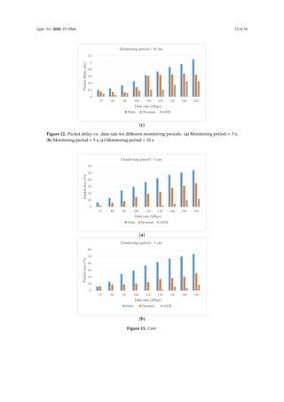
Figure 13. Packet loss ratio vs. data rate for different monitoring periods. (a) Monitoring period = 3 s;
(b) Monitoring period = 5 s; (c) Monitoring period = 10 s
5. Conclusions
This paper successfully introduces an ANN in the SDN control plane for intelligent path
selection with congestion avoidance. The proposed AIER mechanism not only can alleviate the
impact of monitoring periods with dynamic routing but also can provide learning ability from past
experiences by integrating AI technology. The AIER mechanism consists of three stages: (1) collection
of a set of adequate data for training, (2) establishment of an ANN model in the control plane with
the training data, and (3) application of the ANN model for path selection. After the ANN model is
trained, the controller can perform more suitable path configuration according to the current data
flow traffic and link load. The effectiveness and superiority of our proposed AIER mechanism are
demonstrated by performing simulations on the Mininet simulator. The simulation results show that
the AIER mechanism considerably outperforms static and dynamic routing schemes in terms of
average throughput, packet delay, and packet loss ratio. In future works, we will design an intelligent
routing scheme that considers link breakup between any two OpenFlow switches as feature data,
except for data flow traffic and link load, to enhance the comprehensiveness of the ANN model.
Author Contributions: Conceptualization, Y.-J.W. and W.-S.H.; methodology, Y.-J.W. and P.-C.H.; software,
P.-C.H. and M.-H.C.; validation, Y.-J.W. and P.-C.H.; formal analysis, Y.-J.W., P.-C.H. and W.-S.H.; investigation,
Y.-J.W., P.-C.H., W.-S.H., and M.-H.C.; data curation, P.-C.H.; writing—original draft preparation, Y.-J.W. and
P.-C.H.; writing—review and editing, Y.-J.W.; supervision, W.-S.H.; project administration, W.-S.H.; funding
acquisition, Y.-J.W. and W.-S.H. All authors have read and agreed to the published version of the manuscript.
Funding: This research was funded in part by the Ministry of Science and Technology under the
Grant No. MOST-109-2221-E-992-063. And, the APC was supported in part the USC intramural
project with the Grant No. 109-05-05002-01.
Conflicts of Interest: The authors declare no conflicts of interest.
References
1. Yousaf, F.Z.; Bredel, M.; Schaller, S.; Schneider, F. NFV and SDN—Key technology enablers for 5G
networks. IEEE J. Sel. Areas Commun. 2017, 35, 2468–2478.
2. Mininet. Available online: https://github.com/mininet/mininet (accessed on 30 April 2020).
3. Mostafaei, H.; Lospoto, G.; di Lallo, R.; Rimondini, M.; di Battista, G. SDNetkit: A testbed for experimenting
SDN in multi-domain networks. In Proceedings of the IEEE Conference on Network Softwarization,
Bologna, Italy, 3–7 July 2017; pp. 1–6.
4. Ivey, J.; Yang, H.; Zhang, C.; Riley, G. Comparing a scalable SDN simulation framework built on ns-3 and
DCE with existing SDN simulators and emulators. In Proceedings of the 2016 ACM SIGSIM Conference on
Principles of Advanced Discrete Simulation, Banff, AB, Canada, 15–18 May 2016; pp.153–164.
Figure 13. Packet loss ratio vs. data rate for different monitoring periods. (a) Monitoring period = 3 s;
(b) Monitoring period = 5 s; (c) Monitoring period = 10 s.
5. Conclusions
This paper successfully introduces an ANN in the SDN control plane for intelligent path selection
with congestion avoidance. The proposed AIER mechanism not only can alleviate the impact of
monitoring periods with dynamic routing but also can provide learning ability from past experiences
by integrating AI technology. The AIER mechanism consists of three stages: (1) collection of a set
of adequate data for training, (2) establishment of an ANN model in the control plane with the
training data, and (3) application of the ANN model for path selection. After the ANN model is
trained, the controller can perform more suitable path configuration according to the current data
flow traffic and link load. The effectiveness and superiority of our proposed AIER mechanism are
demonstrated by performing simulations on the Mininet simulator. The simulation results show
that the AIER mechanism considerably outperforms static and dynamic routing schemes in terms of
average throughput, packet delay, and packet loss ratio. In future works, we will design an intelligent
routing scheme that considers link breakup between any two OpenFlow switches as feature data,
except for data flow traffic and link load, to enhance the comprehensiveness of the ANN model.
Author Contributions: Conceptualization, Y.-J.W. and W.-S.H.; methodology, Y.-J.W. and P.-C.H.; software, P.-C.H.
and M.-H.C.; validation, Y.-J.W. and P.-C.H.; formal analysis, Y.-J.W., P.-C.H. and W.-S.H.; investigation, Y.-J.W.,
P.-C.H., W.-S.H., and M.-H.C.; data curation, P.-C.H.; writing—original draft preparation, Y.-J.W. and P.-C.H.;
writing—review and editing, Y.-J.W.; supervision, W.-S.H.; project administration, W.-S.H.; funding acquisition,
Y.-J.W. and W.-S.H. All authors have read and agreed to the published version of the manuscript.
Funding: This research was funded in part by the Ministry of Science and Technology under the Grant No.
MOST-109-2221-E-992-063. And, the APC was supported in part by the USC intramural project with the Grant No.
109-08-01003.
Conflicts of Interest: The authors declare no conflict of interest.
References
1. Yousaf, F.Z.; Bredel, M.; Schaller, S.; Schneider, F. NFV and SDN—Key technology enablers for 5G networks.
IEEE J. Sel. Areas Commun. 2017, 35, 2468–2478. [CrossRef]
2. Mininet. Available online: https://github.com/mininet/mininet (accessed on 30 April 2020).
3. Mostafaei, H.; Lospoto, G.; di Lallo, R.; Rimondini, M.; di Battista, G. SDNetkit: A testbed for experimenting
SDN in multi-domain networks. In Proceedings of the IEEE Conference on Network Softwarization, Bologna,
Italy, 3–7 July 2017; pp. 1–6.
4. Ivey, J.; Yang, H.; Zhang, C.; Riley, G. Comparing a scalable SDN simulation framework built on ns-3 and
DCE with existing SDN simulators and emulators. In Proceedings of the 2016 ACM SIGSIM Conference on
Principles of Advanced Discrete Simulation, Banff, AB, Canada, 15–18 May 2016; pp. 153–164.

Appl. Sci. 2020, 10, 6564 15 of 16
5. Wang, S.Y. Comparison of SDN OpenFlow network simulator and emulators: EstiNet vs. Mininet.
In Proceedings of the IEEE Symposium on Computers and Communications, Funchal, Portugal, 23–26 June
2014; pp. 1–6.
6. Mostafaei, H.; Lospoto, G.; di Lallo, R.; Rimondini, M.; di Battista, G. A framework for multi-provider virtual
private networks in software-defined federated networks. Int. J. Netw. Manag. 2020, e2116. [CrossRef]
7. Gouveia, R.; Aparício, J.; Soares, J.; Parreira, B.; Sargento, S.; Carapinha, J. SDN framework for connectivity
services. In Proceedings of the IEEE International Conference on Communications, Sydney, Australia,
10–14 June 2014; pp. 3058–3063.
8. Benzekki, K.; El Fergougui, A.; Elbelrhiti Elalaoui, A. Software-defined networking (SDN): A survey.
Secur. Commun. Netw. 2016, 9, 5803–5833. [CrossRef]
9. SDN White Paper. Available online: https://www.opennetworking.org/download-after/sdn-transport-
api-interoperability-demonstration-executive-overview-technical-white-paper-download/ (accessed on
28 November 2019).
10. Khan, S.; Gani, A.; Wahab, A.W.A.; Guizani, M.; Khan, M.K. Topology discovery in software defined
networks: Threats, taxonomy, and state-of-the-art. IEEE Commun. Surv. Tutor. 2017, 19, 303–324. [CrossRef]
11. McKeown, N.; Anderson, T.; Balakrishnan, H.; Parulkar, G.; Peterson, L.; Rexford, J.; Shenker, S.; Turner, J.
OpenFlow: Enabling innovation in campus networks. ACM SIGCOMM Comput. Commun. Rev. 2008, 38,
69–74. [CrossRef]
12. Open Networking Foundation (ONF). Available online: https://www.opennetworking.org/ (accessed on 28
November 2019).
13. Shoham, Y.; Perrault, R.; Brynjolfsson, E.; Clark, J.; Manyika, J.; Niebles, J.C.; Lyons, T.; Etchemendy, J.;
Grosz, B.; Bauer, Z. AI Index 2018 Report; Stanford University: Stanford, CA, USA, 2018.
14. Turing, A.M. Computing machinery and intelligence. Mind 1950, 59, 433–460. [CrossRef]
15. Searle, J. Minds, brains and programs. Behav. Brain Sci. 1980, 3, 417–457. [CrossRef]
16. Difference between Artificial Intelligence, Machine Learning, Deep Learning. Available online: https://blogs.
nvidia.com.tw/2016/07/whats-difference-artificial-intelligence-machine-learning-deep-learning-ai/ (accessed
on 6 January 2020).
17. Cortes, C.; Vapnik, V. Support-vector network. Mach. Learn. 1995, 20, 273–297. [CrossRef]
18. Quinlan, J.R. Induction of decision trees. Mach. Learn. 1986, 1, 81–106. [CrossRef]
19. Ho, T.K. Random decision forests. In Proceedings of the 3rd International Conference on Document Analysis
and Recognition, Montreal, QC, Canada, 14–16 August 1995; Volume 1, pp. 278–282.
20. McCulloch, W.S.; Pitts, W. A logical calculus of the ideas immanent in nervous activity. Bull. Math. Biophys.
1943, 5, 115–133. [CrossRef]
21. Han, T.; Jiang, D.; Zhao, Q.; Wang, L.; Yin, K. Comparison of random forest, artificial neural networks and
support vector machine for intelligent diagnosis of rotating machinery. Trans. Inst. Meas. Control 2018, 40,
2681–2693. [CrossRef]
22. Rumelhart, D.E.; Hinton, G.E.; Williams, R.J. Learning representations by back-Propagating errors. Nature
1986, 323, 533–536. [CrossRef]
23. James, F.K.; Keith, W.R. Computer Networking: A Top-Down Approach; Pearson Education Limited: London, UK,
2016.
24. Dijkstra, E. A note on two problems in connexion with graphs. Numer. Math. 1959, 1, 269–271. [CrossRef]
25. Jiang, J.R.; Huang, H.W.; Liao, J.H.; Chen, S.Y. Extending Dijkstra’s shortest path algorithm for software
defined networking. In Proceedings of the 16th Asia-Pacific Network Operations and Management
Symposium, Hsinchu, Taiwan, 17–19 September 2014; pp. 1–4.
26. Cheocherngngarn, T.; Jin, H.; Andrian, J.; Pan, D.; Liu, J. Depth-First Worst-Fit search based multipath
routing for data center networks. In Proceedings of the IEEE Global Communications Conference, Anaheim,
CA, USA, 3–7 December 2012; pp. 2821–2826.
27. Lan, Y.U.; Wang, K.; Hsu, Y.I. Dynamic load-balanced path optimization in SDN-based data center networks.
In Proceedings of the 10th International Symposium on Communication Systems, Networks and Digital
Signal Processing, Prague, Czech Republic, 20–22 July 2016; pp. 1–6.
28. Song, S.; Lee, J.; Son, K.; Jung, H.; Lee, J. A congestion avoidance algorithm in SDN environment.
In Proceedings of the International Conference on Information Networking, Kota Kinabalu, Malaysia,
13–15 January 2016; pp. 420–423.

Appl. Sci. 2020, 10, 6564 16 of 16
29. Kao, M.; Huang, B.; Kao, S.; Tseng, H. An effective routing mechanism for link congestion avoidance in
software-defined networking. In Proceedings of the International Computer Symposium, Chiayi, Taiwan,
15–17 December 2016.
30. IEEE Standard 802.1AB-2009 (Cor2 2015). Available online: https://standards.ieee.org/standard/ (accessed on
28 June 2020).
31. Akin, E.; Korkmaz, T. Comparison of routing algorithms with static and dynamic link cost in SDN-extended
version. In Proceedings of the 16th IEEE Annual Consumer Communications Networking Conference,
Las Vegas, NV, USA, 11–14 January 2019; pp. 1–8.
32. Yao, H.; Mai, T.; Jiang, C.; Kuang, L.; Guo, S. AI routers network mind: A hybrid machine learning
paradigm for packet routing. IEEE Comput. Intell. Mag. 2019, 14, 21–30.
33. Chen, Z.; Chen, M.; Zhu, Y.; Huang, H.; Ai, C. A high-throughput routing protocol for wireless sensor
networks. In Proceedings of the 4th IEEE International Conference on Information Science and Technology,
Shenzhen, China, 26–28 April 2014; pp. 710–713.
34. Ai-Zubi, R.T.; Abedsalam, N.; Atieh, A.; Darabkh, K.A. Lifetime-improvement routing protocol for wireless
sensor networks. In Proceedings of the 15th International Multi-Conference on Systems, Signals Devices,
Hammamet, Tunisia, 19–22 March 2018; pp. 683–687.
35. Zhang, F.; Yin, Z.; Gu, A.; Li, Y.; Liu, H. Research on simulation of cluster routing protocol for industrial
wireless sensor networks. In Proceedings of the IEEE 4th International Conference on Computer and
Communications, Chengdu, China, 7–10 December 2018; pp. 265–269.
36. Sendra, S.; Rego, A.; Lloret, J.; Jimenez, J.M.; Romero, O. Including artificial intelligence in a routing protocol
using software defined networks. In Proceedings of the IEEE International Conference on Communications
Workshops, Paris, France, 21–25 May 2017; pp. 670–674.
37. Pasca, S.T.V.; Kodali, S.S.P.; Kataoka, K. AMPS: Application aware multipath flow routing using machine
learning in SDN. In Proceedings of the 23rd National Conference on Communications, Chennai, India,
2–4 March 2017; pp. 1–6.
38. Fu, Q.; Sun, E.; Meng, K.; Li, M.; Zhang, Y. Deep Q-learning for routing schemes in SDN-based data center
networks. IEEE Access 2020, 8, 103491–103499. [CrossRef]
39. Ryu. Available online: https://github.com/faucetsdn/ryu/ (accessed on 30 April 2020).
40. Khan, S.; Bagiwa, M.A.; Wahab, A.W.A.; Gani, A.; Abdelaziz, A. Understanding link fabrication attack in
software defined network using formal methods. In Proceedings of the IEEE International Conference on
Informatics, IoT, and Enabling Technologies, Doha, Qatar, 2–5 February 2020; pp. 555–562.
41. Iperf. Available online: https://iperf.fr/ (accessed on 8 May 2020).
42. Hinton, G.; Salakhutdinov, R. Reducing the dimensionality of data with neural networks. Science 2006, 313,
504–507. [CrossRef] [PubMed]
© 2020 by the authors. Licensee MDPI, Basel, Switzerland. This article is an open access
article distributed under the terms and conditions of the Creative Commons Attribution
(CC BY) license (http://creativecommons.org/licenses/by/4.0/).

9-2020.pdf

Recommended

Recommended

More Related Content

Similar to 9-2020.pdf

Similar to 9-2020.pdf (20)

Recently uploaded

Recently uploaded (10)

9-2020.pdf