4.1 Handling data conv.docx

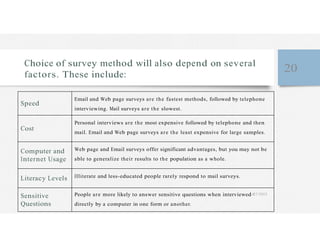
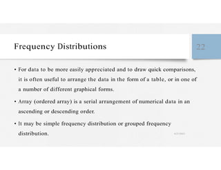
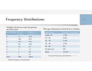
Data handling 1
Atoma Negera (MPH)
4/27/2023

Introduction 2
• Statistics is a field of study concerned with:
1. the collection, organization, summarization, and analysis of data; and
2. the drawing of inferences about a body of data when only a part of the
data is observed.
• Biostatistics: when the tools of statistics are employed on the data
derived from the biological sciences and medicine or public health, we
use the term biostatistics 4/27/2023

Variable 3
• Data are numbers which can be measured or can be obtained by counting
• Variable: A characteristic which takes different values in different
persons, places, or things.
• Any aspect of an individual or object that is measured (e.g., BP) or recorded
(e.g., age, sex) and takes any value.
• There may be one variable in a study or many.
E.g., A study of treatment outcome of TB 4/27/2023

Variable… 4
• Variables can be broadly classified into:
• Categorical (Qualitative)
• can not be measured in quantitative form but can only be sorted by name
or categories
• The notion of magnitude is absent or implicit.
• Numerical (Quantitative) variables
• A variable that can be measured or counted and expressed numerically.
4/27/2023
• Has the notion of magnitude.

Variable… 5
Quantitative variable is divided into two:
1. Discrete: It can only have a limited number of discrete values (usually whole
numbers).
• E.g., the number of episodes of diarrhoea a child has had in a year. You can’t
have 12.5 episodes of diarrhoea
• Characterized by gaps or interruptions in the values (integers).
• Both the order and magnitude of the values matter.
4/27/2023
• The values aren’t just labels, but are actual measurable quantities.

Variable… 6
2. Continuous variable: It can have an infinite number of possible values
in any given interval.
• Both the magnitude and the order of the values matter
• Does not possess the gaps or interruptions
• Weight is continuous since it can take on any number of values (e.g.,
34.575 Kg).
4/27/2023

Summary of variables
Variable
7
Types of
variables
Qualitative
or categorical
Quantitative
measurement
Nominal
(not ordered)
E.g. Ethnic group
Ordinal
(ordered)
E.g. Response to
treatment
Discrete
(count data)
E.g. # Of
admissions
Continuous
(real-valued)
E.g. Height
4/27/2023
Measurement scales

Scales of measurement… 8
1. Nominal scale
The simplest type of data, in which the values fall into unordered categories or
classes
Consists of “naming” observations or classifying them into various mutually
exclusive and collectively exhaustive categories
Uses names, labels, or symbols to assign each measurement.
• Examples: Blood type, sex, race, marital status, etc.
• The numbers have no meaning 4/27/2023
• They are labels only

2. Ordinal scale
• Assigns each measurement to one of a limited number of categories that
are ranked in terms of order.
• Although non-numerical, can be considered to have a natural ordering
• Examples: Patient status, cancer stages, social class, etc.
• The numbers have LIMITED meaning 4>3>2>1 is all we know apart from their
utility as labels 4/27/2023

3. Interval scale
• Measured on a continuum and differences between any two numbers on a
scale are of known size.
Example: Temp. in o
F on 4 consecutive days
Days: Mon Tue Wed Thu
Temp. o
F: 50 55 60 65
• For these data, not only is Monday with 50o cooler than Thursday with 65o, but is 15o
cooler.
• It has no true zero point. “0” is arbitrarily chosen and doesn’t reflect the
absence of temp.

4. Ratio scale
• Measurement begins at a true zero point and the scale has equal space.
- Examples: Height, age, weight, BP, etc.
• Note on meaningfulness of “ratio”-
• Someone who weighs 80 kg is two times as heavy as someone else who weighs
40 kg. This is true even if weight had been measured in other measurements.
4/27/2023

Degree
of
precision
in
measuring
Nominal
Ordinal
Interval
Ratio 4/27/2023

Types and Methods of Data Collection 13
• The statistical data may be classified under two categories depending up
on the sources:
1. Primary Data: are those data which are collected by the investigator
himself for the purpose of a specific inquiry or study.
2. Secondary Data: when an investigator uses data which have already
been collected by others.
4/27/2023

Data collection methods 14
1. Observation
• It is a technique that involves systematically selecting, watching, and recording
behaviors of people, measuring characteristics or other phenomena.
• It includes all methods from simple visual observations to the use of high level
machines.
• Advantage: Gives relatively more accurate data on behavior and activities.
• Disadvantages: observer’s own bias, prejudice, desires may be reflected and needs
more resources and skilled human power during the use of high level machines.

2 . Self-administered Questionnaire & Interviews 15
• These are the most commonly used research data collection techniques.
• Self-administered questionnaire is
• simpler and cheaper
• can be administered to many persons simultaneously
• can be sent by post (unlike interviews)
• But requires a certain level of education and skill on the part of the respondents
• People of a low socio-economic status are less likely to respond 4/27/2023

3. Face-to-face and telephone interviews 16
• An interview is a conversation for gathering information. Involves an
interviewer, who coordinates the process of the conversation and asks questions,
and an interviewee, who responds to those questions.
• A good interviewer can stimulate and maintain the respondent’s interest, and
can create a rapport (understanding) and atmosphere conducive to the
answering of questions.
• If anxiety aroused, the interviewer can allay it. If a question is not understood
an interviewer can repeat it and explain. 4/27/2023

4. Mailed Questionnaire Method 17
• The investigator prepares a questionnaire pertaining to the field of inquiry and
are sent by post to the informants together with a polite covering letter
explaining the detail, the aims and objectives of collecting the information.
• Requests the respondents to cooperate by furnishing the correct replies and
returning the questionnaire duly filled in
• Drawback: response rates tend to be relatively low, and there may be
under representation of less literate subjects
4/27/2023

5. Use of Documentary Sources 18
• Includes clinical and other personal records, death certificates, published
mortality statistics, census publications, etc.
• Examples:
Official publications of CSA
Publication of MoH and other Ministries
Newspapers and Journals
International publications (WHO, UNICEF)
4/27/2023
Records of Hospitals or any HI

The selection of the method of data collection is also
based on practical considerations, such as: 19
The need for personnel, skills, equipment, etc. into what is available
and the urgency with which results are needed.
The acceptability of the procedures to the subjects – the absence of
inconvenience, unpleasantness, or untoward
The probability that the method will provide a good coverage, i.e. will
supply the required information about all or almost all members of the
population or sample
4/27/2023

Choice of survey method will also depend on several
factors. These include:
20
Speed
Cost
Computer and
Internet Usage
Literacy Levels
Sensitive
Questions
Email and Web page surveys are the fastest methods, followed by telephone
interviewing. Mail surveys are the slowest.
Personal interviews are the most expensive followed by telephone and then
mail. Email and Web page surveys are the least expensive for large samples.
Web page and Email surveys offer significant advantages, but you may not be
able to generalize their results to the population as a whole.
Illiterate and less-educated people rarely respond to mail surveys.
People are more likely to answer sensitive questions when interviewed /27/2023
directly by a computer in one form or another.

Presenting and summarizing data 21
4/27/2023

Frequency Distributions 22
• For data to be more easily appreciated and to draw quick comparisons,
it is often useful to arrange the data in the form of a table, or in one of
a number of different graphical forms.
• Array (ordered array) is a serial arrangement of numerical data in an
ascending or descending order.
• It may be simple frequency distribution or grouped frequency
distribution. 4/27/2023

Frequency Distributions 23
Number of movies seen by person
on television The age of persons arrested in a country
No. of movies
0
1
2
3
4
5
6
No. of
persons
72
106
153
40
18
7
3
Relative
frequency (%)
18.0
26.5
38.3
10.0
4.5
1.8
0.8
Age (years)
Under 18
18 – 24
25 – 34
35 – 44
45 – 54
55 and over
Total
Number of persons
1,748
3,325
3,149
1,323
512
335
10,392
7 1 0.3
Total 400 100.0
Grouped frequency distribution 4/27/2023
Simple frequency distribution

K
Construction of grouped frequency distribution 24
Grouped data frequency distribution
• To determine the number of class intervals and the corresponding width, we
may use:
Sturge’s rule: K 1 3.322(log(n))
W
L S
where K = number of class intervals n = no. of observations
W = width of the class interval L = the largest value
S = the smallest value
4/27/2023

Example 25
• Leisure time (hours) per week for 40 college
students:
Time Freque
(Hours) ncy
Relative
Frequency
Cumulative
Relative
23 24 18 14 20 36 24 26 23 21
16 15 19 20 22 14 13 10 19 27
29 22 38 28 34 32 23 19 21 31
16 28 19 18 12 27 15 21 25 16
10-14 5
15-19 11
20-24 12
25-29 7
Frequency
12.5 12.5
27.5 40.0
30.0 70.0
17.5 87.5
K = 1 + 3.322 (log40) = 6.32 ≈ 6
• Max. value = 38, Min. value = 10
• Width = (38-10)/6 = 4.66 ≈ 5
30-34 3
35-39 2
Total 40
7.5 95.0
5.0 100.0
100.0
4/27/2023

Data organization: Tables 26
• The use of tables for presenting data involves grouping the data into mutually
exclusive categories of the variable, and counting the number of occurrences to
each category
• Tables should be as simple as possible and self-explanatory
• Table title should be placed above the table.
• Totals should be shown either in the top row and the first column or in the last row
and last column
• If data are not original, their source should be given in a footnote 4/27/2023

Presenting and summarizing data 27
Specific types of graphs include:
• Bar graph
• Pie chart
• Histogram
• Stem-and-leaf plot
• Box plot
• Scatter plot
• Line graph
• Others
Nominal, ordinal
data
Quantitative
data
4/27/2023

.
t
1. Bar charts (graphs) 28
• Categories are listed on the horizontal axis (X-
axis)
• Frequencies or relative frequencies are
represented on the Y-axis (ordinate)
Bar chart of 25 ICU admitted
patients
14
12
10
8
6
4
2
• The height of each bar is proportional to the 0
Medical Surgical Cardiac Other
frequency or relative frequency of observations in
that category
Medical case
4/27/2023

.
at
e
t
i. Simple Bar chart… 29
• This is a one- dimensional
diagram in which the bar
Distribution of patients in hospital by source
900
of referral
800 769
represents the whole of the
magnitude
• Used for one variable
700
600
500
400
300
200
100
623
256
97
161
0
Other
hospital
GP OPD Casualty /2023 Other
Source of referral

er
e
tage
ii. Multiple bar graph 30
• components are shown as
120
Smoking status Vs presence of asthma
separated bars joining each
other.
• It is used for frequency
distribution of more than
one variable
100 91.4
80
60
40
20 8.6
0
Never smoker
91.7
8.3
Ex-smoker
95.9
4.1
Current smoker
• We can see from the graph quickly that the
prevalence of the asthma decreases with the
smoking.
Smoking status
No asthma Asthma 4/27/2023

iii. Component (Sub-divided) bar chart 31
• When bars are sub-divided in to components parts of the figure
• These sorts of diagram are constructed when each total is built up
from two or more component figures
• The order in which the components are shown in a “bar” is followed
in all bars used in the diagram.
• Example: Stacked and 100% Component bar charts
4/27/2023

.
at
ent
Example: Plasmodium species distribution for confirmed malaria
cases, Z woreda, 2020 32
20
15
10
5
0
September October November December
Year of 2020
P. falciparum p. vivax mixed
4/27/2023

2. Pie chart 33
• Shows the relative frequency for each category by dividing a circle into
sectors, the angles of which are proportional to the relative frequency.
• Used for a single categorical variable
• Use percentage distributions
Relative frequency
0.50
0.25
p
Size of wedge, in degrees
50% of 360 = 180 degrees
25% of 360 = 90 degrees
4/27/2023
P * 100% * 360 degrees

Pie-chart – smoking status (%) 34
Current smoker
18%
Smoking status
Never smokers
Ex-smokers
Current smokers
Relative frequency
54%
28%
18%
Ex-smoker
28%
Never smoker
54%
4/27/2023

3. Histogram 35
• Histograms are frequency distributions with continuous class intervals
that have been turned into graphs.
• Non-overlapping intervals that cover all of the data values must be used.
• Bars are drawn over the intervals in such a way that the areas of the
bars are all proportional in the same way to their interval frequencies.
• The area of each bar is proportional to the frequency of observations in
the interval
4/27/2023

Example: Distribution of the age of women at the time of marriage
Age group 15-20 21-25
Number 13 19
26-30 31-35
32 14
36-40 41-45 46-50
7 3 2
36
4/27/2023

4. Stem-and-Leaf Plot 37
• A quick way to organize data to give visual impression similar to a
histogram while retaining much more detail on the data.
• Similar to histogram and serves the same purpose and reveals the
presence or absence of symmetry
• Are most effective with relatively small data sets
• Are not suitable for reports and other communications, but help
researchers to understand the nature of their data 4/27/2023

Example 38
43, 28, 34, 61, 77, 82, 22, 47, 49, 51, 29, 36, 66, 72, 41
2 2 8 9
3 4 6
4 1 3 7 9
5 1
6 1 6
7 2 7
8 2
4/27/2023

Example: 3031, 3101, 3265, 3260, 3245, 3200, 3248, 3323, 3314, 3484,
3541, 3649 (BWT in g) 39
Stem Leaf
30 31
31 01
32 65 60 45 00 48
33 23 14
34 84
35 41
36 49
Number
1
1
5
2
1
1
1
4/27/2023

5. Frequency polygon 40
• A frequency distribution can be portrayed graphically in yet another way by
means of a frequency polygon.
• To draw a frequency polygon we connect the mid-point of the tops of the
cells of the histogram by a straight line.
• The total area under the frequency polygon is equal to the area under the
histogram
• Useful when comparing two or more frequency distributions by drawing them
on the same diagram
4/27/2023

Frequency polygon for the ages of 2087 mothers with <5 children,
Adami Tulu, 2003
41
700
600
500
400
300
200
100
0
15.0 20.0 25.0 30.0 35.0 40.0 45.0 50.0
Std. Dev = 6.13
Mean = 27.6
N = 2087.00
55.0
N1AGEMOTH 4/27/2023

o
o
o
en
• It can be also drawn without erecting rectangles by joining the top
midpoints of the intervals representing the frequency of the classes
as follows:
42
Age of women at the time of marriage
40
35
30
25
20
15
10
5
0
12 17 22 27 32
Age
37 42 47
4/27/2023

6. Ogive Curve (The Cumulative Frequency Polygon) 43
• Some times it may be necessary to know the number of items whose values are
more or less than a certain amount.
• E.g: we may be interested to know the no. of patients whose weight is <50 Kg or >60 Kg.
• To get this information it is necessary to change the form of the frequency
distribution from a ‘simple’ to a ‘cumulative’ distribution.
• Ogive curve turns a cumulative frequency distribution in to graphs.
• Are much more common than frequency polygons 4/27/2023

Cumulative Frequency and Cum. Rel. Freq. of Age of
25 ICU Patients 44
Age
Interval
10-19
20-29
30-39
40-49
50-59
60-69
70-79
80-89
Total
Frequen
cy
3
1
3
0
6
1
9
2
25
Relative
Frequen
cy (%)
12
4
12
0
24
4
36
8
100
Cumulative
frequency
3
4
7
7
13
14
23
25
Cumulative
Rel. Freq.
(%)
12
16
28
28
52
56
92
100
4/27/2023

7. Line graph 45
• Useful for assessing the trend of particular situation overtime.
• Helps for monitoring the trend of epidemics.
• The time, in weeks, months or years, is marked along the horizontal axis, and
values of the quantity being studied is marked on the vertical axis.
• Values for each category are connected by continuous line.
• Sometimes two or more graphs are drawn on the same graph taking the same
scale so that the plotted graphs are comparable.
4/27/2023

o.
o
con
rmed
ma
ar
a
c
a
s
e
s
No. of microscopically confirmed malaria cases by species and month at
Batu malaria control unit, 2003
46
21 00
18 00 P o sitive
15 00 P . falciparu m
P . vivax
12 00
900
600
300
0
J a n Fe b Mar Apr Ma y J u n J ul Aug S e p Oc t Nov De c
M o n th s
4/27/2023

General rules for constructing graphs 47
• Every graph should be self-explanatory and as simple as possible
• Titles are usually placed below the graph
• Legends or keys should be used to differentiate variables if >1 is shown
• The axes label should be placed to read from the left side and from the bottom
• The units into which the scale is divided should be clearly indicated
• The numerical scale representing frequency must start at zero or a break in the
line should be shown 4/27/2023

Data summarization 48
4/27/2023

1. Measures of Central Tendency (MCT) 49
• The objective of calculating MCT is to determine a single figure which may be
used to represent the whole data set. So that facilitates comparison within one
group or between groups of data.
• Since this stage is usually in the centre of distribution, the tendency of the
statistical data to get concentrated at a certain value is called “central
tendency”
• The various methods of determining the point about which the observations tend
to concentrate are called MCT.
4/27/2023

1. Measures of Central Tendency… 50
Position
2 0
1 5
1 0
5
0 4/27/2023
0-9 10-1 9 20 -2 9 30 -3 9 40 -49 50 -5 9 60 -6 9 70 -7 9 8 0-8 9 9 0-99

1. Arithmetic Mean 51
A. Ungrouped Data
• The arithmetic mean is the "average" of the data set and by far the most
widely used measure of central location
• Is the sum of all the observations divided by the total number of
observations.
4/27/2023

1. Arithmetic Mean… 52
• - the Greek symbol sigma says ‘add up some items’
• - below the sigma symbol is the starting point
• - up top is the ending point
For example,
• Instead of writing x1+x2+x3+x4+x5
• We write � 4/27/2023

�
� �
Arithmetic mean for ungrouped data… 53
• Mean ( ) =
∑�
�
��
=
(�� ⋯ ��)
• The heart rates for n=10 patients were as follows (beats per minute):
167, 120, 150, 125, 150, 140, 40, 136, 120, 150
• What is the arithmetic mean for the heart rate of these patients?
• ( ) =
∑
=
=129.8 beats per minute
4/27/2023

�
�
�
1. Arithmetic Mean… 54
B) grouped data
• In calculating the mean from grouped data, we assume that all values
falling into a particular class interval are located at mid-point of the
interval. It is calculated as follow:
Mean (
Where, k – number of class intervals
) =
∑� �
��
� � �
mi – mid-point of the ith class intervals 4/27/2023
fi – frequency of the ith class intervals

Example: Compute the mean age of 169 subjects from the grouped
data. 55
Class interval
10-19
20-29
30-39
40-49
50-59
60-69
Total
Mid-point (mi)
14.5
24.5
34.5
44.5
54.5
64.5
__
Frequency mifi
(fi)
4 58.0
66 1617.0
47 1621.5
36 1602.0
12 654.0
4 258.0
169 5810.5
Mean ( ) =
∑
∑
=
5810.5
169
= 34.48 years 4/27/2023

Properties of the Arithmetic Mean. 56
• For a given set of data there is one and only one arithmetic mean
(uniqueness).
• Easy to calculate and understand (simple).
• Influenced by each and every value in a data set
• Greatly affected by the extreme values.
• In case of grouped data if any class interval is open, arithmetic mean
can not be calculated. 4/27/2023

2. Median 57
a) Ungrouped data
• The median is the value which divides the data set into two equal parts.
• If the number of values is odd, the median will be the middle value when all
values are arranged in order of magnitude.
• When the number of observations is even, there is no single middle value but
two middle observations.
• In this case the median is the mean of these two middle observations, when all
observations have been arranged in the order of their magnitude.
4/27/2023

2. Median … 61
• The median is a better description (than the mean) of the majority
when the distribution is skewed
• Example
• Data: 14, 89, 93, 95, 96
• Skewness is reflected in the outlying low value of 14
• The sample mean is 77.4
• The median is 93
4/27/2023

b) Grouped data 62
• In calculating the median from grouped data, we assume that the values
within a class-interval are evenly distributed through the interval.
• The first step is to locate the class interval in which the median is located,
using the following procedure.
• Find n/2 and see a class interval with a minimum cumulative frequency which
contains n/2.
• Then, use the following formal.
4/27/2023

~
2. Median … 63
x = L m
where,
n
2 Fc
f m
W
Lm = lower true class boundary of the interval containing the median
Fc = cumulative frequency of the interval just above the median class interval
fm = frequency of the interval containing the median
W= class interval width 4/27/2023

n = total number of observations

Example: Compute the median age of 169 subjects from the
grouped data. 64
n/2 = 169/2 = 84.5
Class
interval
10-19
20-29
30-39
40-49
50-59
Mid-point
(mi)
14.5
24.5
34.5
44.5
54.5
Frequency Cum.
(fi) freq
4 4
66 70
47 117
36 153
12 165
• n/2 = 84.5 = in the 3rd class interval
• Lower limit = 29.5, Upper limit = 39.5
• Frequency of the class = 47
• (n/2 – fc) = 84.5-70 = 14.5
• Median = 29.5 + (14.5/47)10 = 32.58
60-69 64.5 4 169 ≈ 33
4/27/2023
Total 169

Properties of the median 65
• There is only one median for a given set of data (uniqueness)
• The median is easy to calculate
• Median is a positional average and hence it is insensitive to very large or very
small values
• Median can be calculated even in the case of open end intervals
• It is determined mainly by the middle points and less sensitive to the remaining
data points (weakness). 4/27/2023

3. Mode 66
• The mode is the most frequently occurring value among all the
observations in a set of data.
• It is not influenced by extreme values.
• It is possible to have more than one mode or no mode.
• It is not a good summary of the majority of the data.
4/27/2023

67
Mode
20
18
16
14
12
10
8
6
4
2 4/27/2023
0
T. Ancelle, D. Coulombie

a) Ungrouped data 68
• It is a value which occurs most frequently in a set of values.
• If all the values are different there is no mode, on the other hand,
a set of values may have more than one mode.
4/27/2023

Example 69
• Data are: 1, 2, 3, 4, 4, 4, 4, 5, 5, 6
• Mode is 4 “Unimodal”
• Data are: 1, 2, 2, 2, 3, 4, 5, 5, 5, 6, 6, 8
• There are two modes – 2 & 5
• This distribution is said to be “bi-modal”
• Data are: 2.62, 2.75, 2.76, 2.86, 3.05, 3.12
• No mode, since all the values are different 4/27/2023

b) Grouped data 70
• To find the mode of grouped data, we usually refer to the modal
class, where the modal class is the class interval with the highest
frequency.
• If a single value for the mode of grouped data must be specified, it is
taken as the mid-point of the modal class interval.
4/27/2023

Properties of mode 72
It is not affected by extreme values
It can be calculated for distributions with open end classes
Often its value is not unique
The main drawback of mode is that often it does not exist
4/27/2023

73
(a) Symmetric and unimodal distribution —
Mean, median, and mode should all be
approximately the same
Mean, Median & Mode
(b) Bimodal —Mean and median should be
about the same, but may take a value
that is unlikely to occur; two modes
might be best

Measures of Variation/Dispersion 74
• MCT are not enough to give a clear understanding about the distribution
of the data.
• We need to know something about the variability or spread of the
values —whether they tend to be clustered close together, or spread
out over a broad range
• Dispersion of a set of observations refers to the scatteredness of
observations around a measure of central tendency 4/27/2023

Measures of Dispersion 75
• Consider the following two sets of data:
A: 177 193 195 209 226 Mean = 200
B: 192 197 200 202 209 Mean = 200
• Two or more sets may have the same mean and/or median
but they may be quite different.
These two distributions have the
same mean, median, and mode
4/27/2023

Measures of dispersion include: 76
1. Range
2. Inter-quartile range
3. Variance
4. Standard deviation
5. Coefficient of variation
6. Standard error 4/27/2023

1. Range (R) 77
• The difference between the largest and smallest observations in a
sample.
Range = Maximum value – Minimum value
• Example –
• Data values: 5, 9, 12, 16, 23, 34, 37, 42
• Range = 42-5 = 37
• Data set with higher range exhibit more variability
4/27/2023

Properties of range 78
It is the simplest crude measure and can be easily understood
It takes into account only two values which causes it to be a poor measure
of dispersion
Very sensitive to extreme observations
The larger the sample size, the larger the range
4/27/2023

2. Variance ( 2, s2) 79
• The main objection of mean deviation, that the negative signs are
ignored, is removed by taking the square of the deviations from the
mean.
• The variance is the average of the squares of the deviations taken from
the mean.
• It is squared because the sum of the deviations of the individual
observations of a sample about the sample mean is always 0 4/27/2023

2. Variance … 80
a) Ungrouped data
A sample variance is calculated for a sample of individual values (X1,
X2, …Xn) and uses the sample mean ( ) rather than the population
mean µ.
4/27/2023

Degrees of freedom 81
• In computing the variance there are (n-1) degrees of freedom because
only (n-1) of the deviations are independent from each other
• The last one can always be calculated from the others automatically.
• This is because the sum of the deviations from their mean (Xi-Mean)
must add to zero.
4/27/2023

b) Grouped data 82
( m i x ) 2
f i
S 2 i = 1
f i - 1
i = 1
Where,
mi = the mid-point of the ith class interval
f
x
i
=
=
t
t
h
h
e
e
s
f
a
r
m
eq
p
u
l
e
e
n
m
cy
ea
o
n
f the ith class interval
k = the number of class intervals
4/27/2023

Properties of Variance: 83
• The main disadvantage of variance is that its unit is the square of the
unite of the original measurement values
• The variance gives more weight to the extreme values as compared to
those which are near to mean value, because the difference is squared
in variance.
• The drawbacks of variance are overcome by the standard deviation.
4/27/2023

3. Standard deviation ( , s) 84
• It is the square root of the variance.
• This produces a measure having the same scale as that of the
individual values.
2
and S = S 2
4/27/2023

Following are the survival times of n=11 patients after heart transplant surgery.
85
Calculate the sample variance and SD.
4/27/2023

Example: Compute the variance and SD of the age of 169 subjects from the
grouped data.
86
Class interval (mi) (fi)
10-19 14.5 4
20-29 24.5 66
30-39 34.5 47
40-49 44.5 36
50-59 54.5 12
60-69 64.5 4
Total 169
(mi-Mean)
-19.98
-9-98
0.02
10.02
20.02
30.02
(mi-Mean)2
399.20
99.60
0.0004
100.40
400.80
901.20
1901.20
(mi-Mean)2 fi
1596.80
6573.60
0.0188
3614.40
4809.60
3604.80
20199.22
Mean = 5810.5/169 = 34.48 years
S2 = 20199.22/169-1 = 120.23 4/27/2023
SD = √S2 = √120.23 = 10.96

Properties of SD 87
• The SD has the advantage of being expressed in the same units of
measurement as the mean
• SD is considered to be the best measure of dispersion and is used widely
because of the properties of the theoretical normal curve.
• However, if the units of measurements of variables of two data sets is
not the same, then there variability can’t be compared by comparing the
values of SD. 4/27/2023

Standard deviation (SD) Vs Standard Error (SE) 88
• SD describes the variability among individual values in a given data set
• SE is used to describe the variability among separate sample means
obtained from one sample to another
• We interpret SE of the mean to mean that another similarly conducted
study may give a mean that may lie between SE.
4/27/2023

Standard Error 89
• SD is about the variability of individuals
• SE is used to describe the variability in the means of repeated samples
taken from the same population.
• E.g: imagine 5,000 samples, each of the same size n=11. This would produce
5,000 sample means. This new collection has its own pattern of variability. We
describe this new pattern of variability using the SE, not the SD.
4/27/2023

Example: The heart transplant surgery 90
• n=11, SD=168.89, Mean=161 days
• What happens if we repeat the study? What will our next mean be? Will it be close?
How different will it be? Focus here is on the generalizability of the study findings.
• The behavior of mean from one replication of the study to the next replication is
referred to as the sampling distribution of mean.
• We interpret this to mean that a similarly conducted study might produce an average
survival time that is near 161 days, ±50.9 days.
4/27/2023

4. Coefficient of variation (CV) 91
• When two data sets have different units of measurements, or their
means differ sufficiently in size, the CV should be used as a measure of
dispersion.
• It is the best measure to compare the variability of two series of sets of
observations.
• Data with less coefficient of variation is considered more consistent.
4/27/2023

S
4. Coefficient of variation … 92
CV is the ratio of the SD to the mean multiplied by 100.
CV
x
100
SD Mean CV (%)
SBP
Cholesterol
15mm
40mg/dl
130mm 11.5
200mg/dl 20.0
• “Cholesterol is more variable than systolic blood pressure”
4/27/2023

Probability and Probability
Distributions
93
4/27/2023

Probability 94
• Chance of observing a particular outcome, likelihood of an event
• Assumes a “stochastic” or “random” process: i.e.. the outcome is not
predetermined - there is an element of chance
• An outcome is a specific result of a single trial of a probability experiment.
• Probability theory developed from the study of games of chance like dice and
cards.
• A process like flipping a coin, rolling a die or drawing a card from a deck are
probability experiments. 4/27/2023

Probability… 95
• Event = something that may happen or not when the experiment is performed
• An event either occurs or it does not occur
• Probability of an Event E – a number between 0 and 1 representing the
proportion of times that event E is expected to happen when the experiment
is done over and over again under the same conditions
• Any event can be expressed as a subset of the set of all possible outcomes (S)
S = set of all possible outcomes
4/27/2023
P(S) = 1

Probability… 96
• Probability theory is a foundation for statistical inference, & allows us to
draw conclusions about a population based on information obtained from a
sample drawn from that population.
More importantly probability theory is used to understand:
• About probability distributions: Binomial, Poisson, and Normal Distributions
• Sampling and sampling distributions
• Estimation
• Hypothesis testing
• Advanced statistical analysis
4/27/2023

General rules which apply to any probability
distribution 97
1. Since the values of a probability distribution are probabilities, they
must be numbers in the interval from 0 to 1.
2. Since a random variable has to take on one of its values, the sum of
all the values of a probability distribution must be equal to 1.
4/27/2023

General rules … 98
Example: Check whether the following function can serve as the
probability distribution of an appropriate random variable
f (x)
x 2
12 for x=1, 2, and 3
Substituting the values of x, f(1)=3/12, f(2)=4/12, and f(3)=5/12
Since none of these values is negative or greater than one, and since their
sum 3/12+4/12+5/12 = 1, the given function is a probability distribution

1. Binomial distribution 99
• It is one of the most widely encountered discrete probability
distributions.
• Consider dichotomous (binary) random variable
• Is based on Bernoulli trial
• When a single trial of an experiment can result in only one of two mutually
exclusive outcomes (success or failure; dead or alive; sick or well, male or
female) 4/27/2023

Example 100
• We are interested in determining whether a newborn infant will
survive until his/her 70th birthday
• Let Y represent the survival status of the child at age 70 years
Y= 1 if the child survives and Y= 0 if he/she does not
• The outcomes are mutually exclusive and exhaustive
• Suppose that 72% of infants born survive to age 70 years
P(Y = 1) = p = 0.72 4/27/2023
P(Y = 0) = 1 − p = 0.28

r
The Binomial Distribution 101
• The distribution of the number of successes (r) in n statistically
independent trails, where the probability of success on each trail is P, is
known as the binomial distribution, and has a probability density
function given by:
P(X r)
n
Pr
(1 P)n r
n n!
Where,
r (n
r )! r!
r = 0, 1, 2, …, n
• The mean is np and variance is np(1-p)
4/27/2023

Example: 102
• What is the probability of obtaining 2 boys out of 5 children if the
probability of a boy is 0.51 at each birth and the sexes of successive
children are considered independent random variables?
n=5, p=0.51, 1-p=0.49 and r=2
P(x 2)
2
(0.51)2
(0.49)3
2!3!
(0.51)2
(0.49)3
0.306
4/27/2023

2. Normal distribution 103
• The Normal Distribution also called the Gaussian distribution is the
most important of the distribution in all statistics.
• Variables such as blood pressure, weight, height, serum cholesterol
level, and IQ score
• The normal density is given by:
f
x
1
2
1 x
2 e 2
where x
3.141...and _ e 2.72... 4/27/2023

Characteristics 104
1. It is symmetrical about its mean
2. Mean, median and mode are equal
3. The total area under the curve above the x axis is one square unit
4. One SD from the mean in both directions approximately 68% of the area
5. The height of the curve = 1/ 2
6. The normal distribution is determined by the parameters standard
deviation and mean.
4/27/2023

The Normal Distribution curve 105
σ = σx
μ = μx 4/27/2023

107
Approximately 68% of the a rea under the standard normal curve lies between ±1, 4/27/2023
about 95% between ±2, and about 99% between ±2.5

The standard Normal distribution 108
• A normal distribution with mean 0 and variance 1 will be referred to as a
standard, or unit, normal distribution. This distribution is denoted by
N(0,1).
f(z)
1 2
z2
2π
for - < z < +
• This distribution is symmetrical about 0 (the mean), since f(x)=f(-x). About 68%
of the area under the normal density lies +1 and -1, about 95% lies between +2
and -2, and about 99% lies between +2.5 and -2.5 4/27/2023

�
�
Z- Scores 109
• Assume a distribution has a mean of 70 and a standard deviation of 10.
• How many standard deviation units above the mean is a score of 80?
��
��
��
1
• How many standard deviation units above the mean is a score of 83?
Z =
��
= 1.3
• The number of standard deviation units is called a Z-score or Zvalue. 4/27/2023

Area under normal curve 110
a) What is the probability that z < -1.96?
(1) Sketch a normal curve
(2) Draw a perpendicular line for z = -1.9
(3) Find the a rea in the table
(4) The answer is the a rea to the left of the line
P(z < -1.96) = 0.0250 4/27/2023

111
b) What is the probability that -1.96 < z < 1.96?
The area between the values P(-1.96 < z < 1.96) = .9750 - .0250 =7.9500

112
c) What is the probability that z > 1.96?
• The answer is the area to the right of the line; found by
subtracting table value from 1.0000; P(z > 1.96) =1.0000 - .9750 =
.0250
4/27/2023

Exercise 113
1. Compute P(-1 ≤ Z ≤ 1.5)
Ans: 0.7745
2. Find the area under the SND from 0 to 1.45
Ans: 0.4265
3. Compute P(-1.66 < Z < 2.85)
Ans: 0.9493
4/27/2023

Application of Normal distribution 114
• Example: the diastolic blood pressures of males 35–44 years of age
are normally distributed with µ = 80 mm Hg and σ2 = 144 mm Hg2
σ = 12 mm Hg
• Therefore, a DBP of 80+12 = 92 mm Hg lies 1 SD above the mean
• Let individuals with BP above 95 mm Hg are considered to be
hypertensive
4/27/2023

Example… 115
a. What is the probability that a randomly selected male has a BP above
95 mm Hg?
• P (Z > 95) = P ( x > )
=P (Z > 1.25)
= 0.1056
• Approximately 10.6% of this population would be classified as
4/27/2023
hypertensive

Example… 116
b. What is the probability that a randomly selected male has a DBP
above 110 mm Hg?
Z = = 2.50
P (Z > 2.50) = 0.0062
• Approximately 0.6% of the population has a DBP above 110 mm Hg
4/27/2023

Example… 117
c. What is the probability that a randomly selected male has a DBP
below 60 mm Hg?
Z = = -1.67
P (Z < -1.67) = 0.0475
• Approximately 4.8% of the population has a DBP below 60 mm Hg
4/27/2023

Exercise 118
• Suppose it is know that the height of a population of individual are
approximately normally distributed with a mean of 70 inches and
standard deviation of 3 inches. What is the probability that a person
picked at random from this group will be
a) between 65 and 74 inches tall?
b) greater than 75 inches
c) less than 65 inches
4/27/2023

Solution 119
Step 1: Transform this to standard normal distribution by using
Step 2: Determine the area under the curve bounded by the curve, x-axis
and the two points.
P( a<z<b).
Step 3: Look at the z distribution table for the corresponding value of z.
4/27/2023

Other Distributions 120
Student t-distribution
F- Distribution
2 -Distribution
4/27/2023

Sampling methods and Sample size
estimation 121
4/27/2023

Why sample? 122
• It is usually not cost effective or practicable to collect and examine all
the data that might be available.
• Instead it is often necessary to draw a sample of information from the
whole population to enable the detailed examination required to take
place.
• Sampling provides a means of gaining information about the population
without the need to examine the population in its entirely.
4/27/2023

Purposes of sampling 123
• Provides various types of statistical information of a qualitative or
quantitative nature about the whole by examining a few selected units.
• Advantages of sample based studies
• Cost effectiveness
• Timeliness
• Inaccessibility of some people
• Less destructive in data summarization 4/27/2023
• Accuracy

Definition of terms 124
• Sample – Subset of the population of interest
• Sampling – process of selecting units from the population of interest so
that by studying the sample we generalize our result back to population.
• Sampling can provide a valid, defensible methodology but it is important
to match the type of sample needed to the type of analysis required.
4/27/2023

Definition of terms… 125
• Population - Finite or infinite set of objects whose properties are to be
studied.
• Study population/sample population – subset of target population
chosen so as to be representative of the total population
• Sampling unit - unit of selection in the sampling process.
• Study unit – subject on which information is collected. 4/27/2023

Sample size estimation 126
• How many subjects are needed in the sample to enable draw conclusion
on the whole population?
• Minimum sample size can be calculated depending on the objective of
the study
• Descriptive studies - Prevalence, coverage and utilization rate studies
• Analytic studies - comparative cross-sectional, case-control, cohort and
clinical trials 4/27/2023

�
�
Sample size - single proportion 127
• For making confidence limit statement (such as prevalence study), the
following formula can be used to estimate minimum sample size:
n
2
Z1
2
P
1 2
P
• For population <10,000, use finite population correction
n f
N Z1
2
2
P 1 P
d 2
N 1 Z1
2
2
P
1 P
�
�
� �
4/27/2023

Parameters in the formula 128
• n is minimum sample size
• P is estimate of the prevalence rate for the population
• From available data, or Pilot study result, or 0.5 should be used to get the possible
minimum large sample size; if given in range, take the value closest to 0.5.
• d is the margin of sampling error tolerated
• Z1- /2 is the standard normal variable at (1- )% confidence level. Usually
95% confidence level is used = 1.96
4/27/2023
• N population size

Exercise 129
• A student want to conduct a research on the prevalence of ANC utilization of
mothers in Mattu town. Given that the prevalence from the previous study
found to be 45.7%, what will be the sample size he should take to address his
objective at 95% CI? Margin of error d= 5%
• A confidence level of 95% will give the value of as Zα/2=1.96.
• Then using the formula of: n =
(
/
) ∗ ( )
• n=382
4/27/2023

Measuring prevalence for more than one item in one
group 130
• Take estimated prevalence of the most important item to be
measured or
• Determine sample size for each item/specific objective and then
• Take estimated prevalence of the item that gives the maximum sample
size
4/27/2023

1
1 1
Sample size-two proportion 131
• For test of significance study the following formula can be used:
Z Z2
2
p 1 p
p2 1 p2 Parameters:
p p2
2
n - size of sample in each group
P1 ,P2 – estimated population prevalence in the comparison groups
β = 1- Power (the probability that if the two proportions differ the test will
produce a significant difference)
4/27/2023
• Usually a power of 80% or 90% is used

Five key factors 132
1. Confidence level: how certain you want to be that the population figure is
within the sample estimate and its associated precision.
2. Variability in the population: the SD is the most usual measure and often
needs to be estimated.
3. Margin of error or precision: a measure of the possible difference between
the sample estimate and the actual population value.
4. The population proportion: the proportion of items in the population
displaying the attributes that you are seeking.
5. Population size: only important if the sample size is greater than 5% of the
population in which case the sample size reduces.
4/27/2023

Sample size – other considerations 133
• Non-response
• Add contingency – say 10%
• More – sensitive topic, self-administered questionnaire (up to 30%)
• Response rate for
• Cross-sectional survey >85%
• Cohort - >60-80%
• Sampling technique
• In complex samples (cluster, multistage) increase the sample size to account for
4/27/2023
design effect

Sampling techniques/methods 134
• Sampling is the process of selecting a number of study units from a defined
study population.
• Clearly define study population and study unit
• Study population
–
individuals, households, institutions, records, etc…
• Study units
–
an individual, a household, an institution or a record
• Types: probability and non-probability
• Probability
–
quantitative studies
4/27/2023
• Non-probability – qualitative studies

Probability sampling technique: 135
• Involves using random selection procedures to ensure that each unit of the
sample is chosen on the basis of chance.
• All units of the study population should have an equal, or at least a known
non-zero chance of being included in the sample.
• Sample drawn in such a way that it is representative of the population
• The type to be used depends on population composition and availability of
sampling frame
4/27/2023

Sampling cont… 136
Probability sampling methods include:
• Simple random sampling
• Systematic sampling
• Stratified sampling
• Cluster sampling
• Multistage sampling
4/27/2023

1. Simple random sampling 137
• Selecting required number of sampling units randomly from list of all units
• Up-to-date Sampling frame
• Random selection – manually using table of random numbers or using
computer programs
• E.g. 250 households from list of 9000 households
• Better representativeness but costly and representativeness reduced in
heterogeneous population
4/27/2023

2. Systematic sampling 138
• Sampling units are selected at regular intervals. The starting unit is selected
randomly
• Example: to select a sample of 100 students from 2500, first calculate sampling
interval = 2500/100 = 25. Then randomly select the first student and finally pick every
25th student
• Easier and less time consuming
• Can be done without sampling frame – sequential studies
• Risk of bias if there is cyclic repetition 4/27/2023

3. Stratified sampling 139
• Used when the population structure consists distinct subgroups/strata
• Ensures proportions of individuals with certain characteristics in the
sample will be the same as those in the whole population
• Representation of groups with different characteristics
• The study population must be divided into strata of the characteristic
(Example: residence, age, sex, profession) and then random or systematic
samples are obtained from each stratum 4/27/2023

3. Stratified sampling ... 140
• Depending on the need, samples from each stratum can be drawn either
proportional to their size or non-proportionally/equal size from each
stratum
• Proportional- using sampling fraction (N/n)
• Equal size – to represent small groups
• Improved representativeness
• Estimates can be obtained for each stratum and the population
4/27/2023

4. Cluster sampling 141
• Groups of study units (clusters) instead of individual study units are selected at a
time
• Assumes homogeneity of population with respect the characteristic to be measured
• All the study units in the selected clusters are included in the study
• Used in geographically scattered areas where visiting dispersed study units is time
consuming and costly
• Example: a simple random sample of 5 villages from 30 villages
• Easier but less representative 4/27/2023

5. Multistage sampling 142
• Carried out in stages – PSU, SSU…
• Used in very large and diverse populations
• The method used in most community-based big studies
• E.g. In a study to be undertaken in a big town the sampling may involve stages like
selection of kefetegnas, kebeles and finally houses
• Representativeness and reduced cost-
• The larger the number of clusters, the greater is the likelihood that the sample will
be representative.
4/27/2023

Bias in sampling 143
• Systematic error – bias in sampling in sampling procedures (lack of representative)
• Non-response - respondents may refuse or forget to fill in the questionnaire
Other sources of bias in sampling:
Studying volunteers only – volunteers are motivated to participate in the study.
Sampling of registered patients only
Seasonal bias.
Tarmac bias – easily accessible by car. 4/27/2023

Bias … 144
There are several ways to reduce the possibility of bias:
1. Data collection tools should be pre-tested.
2. If non-response is due to absence of the subjects, follow-up non-respondents.
3. If non-response is due to refusal to co-operate, an extra, separate study of non-
respondents may be considered in order to identify to what extent they differ from
respondents.
4. Include additional people in the sample, so that non-respondents can be replaced if their
absence was very unlikely to be related to the topic being studied. 4/27/2023

Non-probability sampling methods 145
• Every element in the universe [sampling frame] does not have equal
probability of being chosen in the sample.
a) Convenience sampling
– Drawn at the convenience of the researcher. Common in exploratory research.
– Does not lead to any conclusion
b) Judgmental sampling
– Sampling based on some judgment, gut-feelings or experience of the researcher.
– If inference drawing is not necessary, these samples are quite useful.
4/27/2023

Non-probability sampling methods… 146
c) Quota Sampling
– Each data collector is assigned a fixed quota of subjects to interview; the number
falling into certain categories (like residence, sex, age, etc.) are also fixed.
– On the other hand, the interviewers are free to select anybody they like.
Other non probability sampling methods
• Snowball or chain sampling
• Extreme case sampling
• Maximum variation sampling
• Homogeneous sampling 4/27/2023
• Critical case sampling

4.1 Handling data conv.docx

More Related Content

Similar to 4.1 Handling data conv.docx

Recently uploaded

4.1 Handling data conv.docx