4.Module_2_Chaptjvyfgcgfxfdxhgfxchtfer_3.pptx

2. Uniform-cost search
1
Instead of expanding the shallowest node, uniform-cost search
expands the node n with the lowest path cost g(n). This is done by
storing the frontier as a priority queue ordered by g.
Goal test is applied to a node when it is selected for expansion
because the first goal node that is generated may be on a suboptimal
path
A test is added in case a better path is found to a node currently on
the frontier

Visit https://www.youtube.com/c/sharikatr for my video
lectures
Prepared by Sharika T R, SNGCE
DEPARTMENT OF CSE SNGCE 2

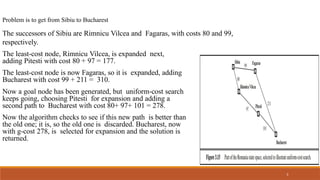
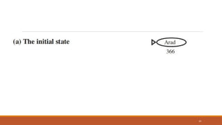
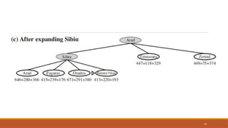
Problem is to get from Sibiu to Bucharest
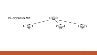
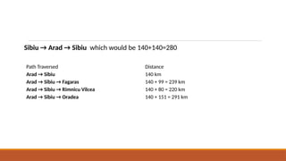
The successors of Sibiu are Rimnicu Vilcea and Fagaras, with costs 80 and 99,
respectively.
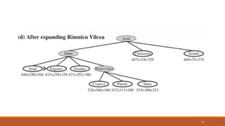
The least-cost node, Rimnicu Vilcea, is expanded next,
adding Pitesti with cost 80 + 97 = 177.
The least-cost node is now Fagaras, so it is expanded, adding
Bucharest with cost 99 + 211 = 310.
Now a goal node has been generated, but uniform-cost search
keeps going, choosing Pitesti for expansion and adding a
second path to Bucharest with cost 80+ 97+ 101 = 278.
Now the algorithm checks to see if this new path is better than
the old one; it is, so the old one is discarded. Bucharest, now
with g-cost 278, is selected for expansion and the solution is
returned.
3

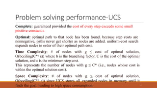
Problem solving performance-UCS
4
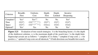
Complete: guaranteed provided the cost of every step exceeds some small
positive constant ε
Optimal: optimal path to that node has been found. because step costs are
nonnegative, paths never get shorter as nodes are added. uniform-cost search
expands nodes in order of their optimal path cost.
Time Complexity: # of nodes with g ≤ cost of optimal solution,
O(bceiling(C*/ ε)) where b is the branching factor, C is the cost of the optimal
solution, and ε is the minimum step cost.
This represents the number of nodes with g ≤ C* (i.e., nodes whose cost is
within the optimal solution cost).
Space Complexity: # of nodes with g ≤ cost of optimal solution,
O(bceiling(C*/ ε)) since UCS stores all expanded nodes in memory until it
finds the goal, leading to high space consumption.

Uniform-cost search is guided by path costs rather than depths, so its complexity is not
easily characterized in terms of b and d.
let C∗ be the cost of the optimal solution and that every action costs at least ε
Then the algorithm’s worst-case time and space complexity is which can be
much greater than bd.
This is because uniform cost search can explore large trees of small steps before
exploring paths involving large and perhaps useful steps.
When all step costs are equal is just bd+1.
When all step costs are the same, uniform-cost search is similar to breadth-first search,
except that bfs stops as soon as it generates a goal, whereas uniform-cost search
examines all the nodes at the goal’s depth to see if one has a lower cost
thus uniform-cost search does strictly more work by expanding nodes at depth d
unnecessarily
5

Depth-first search
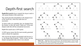
Depth-first search always expands the deepest node in
the current frontier of the search tree.
The search proceeds immediately to the deepest level
of the search tree, where the nodes have no
successors.
As those nodes are expanded, they are dropped from
the frontier, so then the search “backs up” to the next
deepest node that still has unexplored successors.
Depth-first search uses a LIFO queue
A LIFO queue means that the most recently generated
node is chosen for expansion.
This must be the deepest unexpanded node because it
is one deeper than its parent—which, in turn, was the
deepest unexpanded node when it was selected
6

Depth-first search
S
7
A D
B D A E
E B B F
19 19 17
D F B F C E A C G
14
G C
17
G F
15 15 13
G 25
C
E
11

Problem solving performance-DFS
8
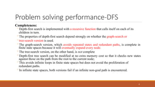
Completeness:
◦Depth-first search is implemented with a recursive function that calls itself on each of its
children in turn.
◦The properties of depth-first search depend strongly on whether the graph-search or
◦tree-search version is used.
◦The graph-search version, which avoids repeated states and redundant paths, is complete in
finite state spaces because it will eventually expand every node.
◦The tree-search version, on the other hand, is not complete
◦Depth-first tree search can be modified at no extra memory cost so that it checks new states
against those on the path from the root to the current node;
◦This avoids infinite loops in finite state spaces but does not avoid the proliferation of
redundant paths.
◦In infinite state spaces, both versions fail if an infinite non-goal path is encountered.

9
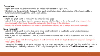
Not optimal
◦Depth- first search will explore the entire left subtree even if node C is a goal node.
◦If node J were also a goal node, then depth-first search would return it as a solution instead of C, which would be a
better solution; hence, depth-first search is not optimal.
Time complexity
◦Depth-first graph search is bounded by the size of the state space
◦A depth-first tree search, on the other hand, may generate all of the O(bm) nodes in the search tree, where m is the
maximum depth of any node; this can be much greater than the size of the state space.
◦m itself can be much larger than d (the depth of the shallowest solution) and is infinite if the tree is unbounded.
Space complexity
◦A depth-first tree search needs to store only a single path from the root to a leaf node, along with the remaining
unexpanded sibling nodes for each node on the path.
◦Once a node has been expanded, it can be removed from memory as soon as all its descendants have been fully
explored.
◦For a state space with branching factor b and maximum depth m, depth-first search requires storage of
only O(bm) nodes.
◦Assuming that nodes at the same depth as the goal node have no successors, we find that depth-first search
would require 156 kilobytes instead of 10 exabytes at depth d = 16, a factor of 7 trillion times less space.

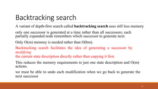
Backtracking search
10
A variant of depth-first search called backtracking search uses still less memory
only one successor is generated at a time rather than all successors; each
partially expanded node remembers which successor to generate next.
Only O(m) memory is needed rather than O(bm).
Backtracking search facilitates the idea of generating a successor by
modifying
the current state description directly rather than copying it first.
This reduces the memory requirements to just one state description and O(m)
actions.
we must be able to undo each modification when we go back to generate the
next successor

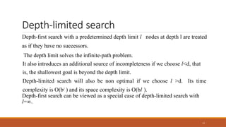
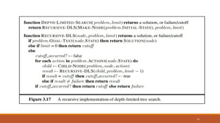
Depth-limited search
11
Depth-first search with a predetermined depth limit l nodes at depth l are treated
as if they have no successors.
The depth limit solves the infinite-path problem.
It also introduces an additional source of incompleteness if we choose l<d, that
is, the shallowest goal is beyond the depth limit.
Depth-limited search will also be non optimal if we choose l >d. Its time
complexity is O(bl ) and its space complexity is O(bl ).
Depth-first search can be viewed as a special case of depth-limited search with
l=∞.

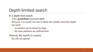
Depth-limited search
12
It is depth-first search
◦with a predefined maximum depth
◦However, it is usually not easy to define the suitable maximum depth
◦too small
◦ no solution can be found too large
◦ the same problems are suffered from
Anyway the search is complete
◦but still not optimal

Depth-limited
search
S
13
A D
B D A E
E B B F
19 19 17
D F B F C E A C G
14
G C G
17
F
15 15 13
G 25
C
E
11
depth = 3
3
6

Iterative deepening depth-
first search
15
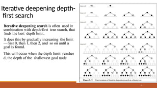
Iterative deepening search is often used in
combination with depth-first tree search, that
finds the best depth limit.
It does this by gradually increasing the limit
—first 0, then 1, then 2, and so on until a
goal is found.
This will occur when the depth limit reaches
d, the depth of the shallowest goal node

◦Because search tree with the same (or nearly the same) branching factor at each level, most of the nodes
are in the bottom level, so it does not matter much that the upper levels are generated multiple times
the nodes on the bottom level (depth d) are generated once, those on the next-to-bottom
level are generated twice, and so on, up to the children of the root, which are generated d
times.
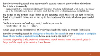
So the total number of nodes generated in the worst case is
◦N(IDS)=(d)b + (d − 1)b2 + ··· + (1)bd ,
which gives a time complexity of O(bd) asymptotically the same as breadth-first search.
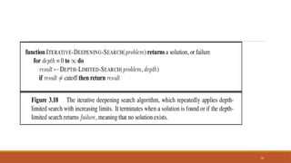
Iterative deepening search is analogous to breadth-first search in that it explores a complete
layer of new nodes at each iteration before going on to the next layer
iterative deepening is the preferred uninformed search method when the search space is
large and the depth of the solution is not known
17
Iterative deepening search may seem wasteful because states are generated multiple times
but it is is not too costly.

18
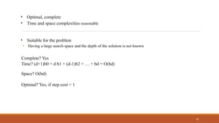
Complete? Yes
Time? (d+1)b0 + d b1 + (d-1)b2 + … + bd = O(bd)
Space? O(bd)
Optimal? Yes, if step cost = 1
• Optimal, complete
• Time and space complexities reasonable
• Suitable for the problem
• Having a large search space and the depth of the solution is not known

INFORMED (HEURISTIC) SEARCH
STRATEGIES
20
Problem-specific knowledge beyond the definition of the problem itself
can find solutions more efficiently than an uninformed strategy

BEST-FIRST SEARCH
21
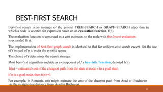
Best-first search is an instance of the general TREE-SEARCH or GRAPH-SEARCH algorithm in
which a node is selected for expansion based on an evaluation function, f(n).
The evaluation function is construed as a cost estimate, so the node with the lowest evaluation
is expanded first.
The implementation of best-first graph search is identical to that for uniform-cost search except for the use
of f instead of g to order the priority queue
The choice of f determines the search strategy.
Most best-first algorithms include as a component of f a heuristic function, denoted h(n):
h(n) = estimated cost of the cheapest path from the state at node n to a goal state.
if n is a goal node, then h(n)=0.
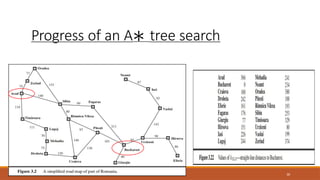
For example, in Romania, one might estimate the cost of the cheapest path from Arad to Bucharest
via the straight-line distance from Arad to Bucharest.

Greedy best-first search
22
Greedy best-first search tries to expand the node that is closest to the goal, on the grounds that this is
likely to lead to a solution quickly.
It evaluates nodes by using just the heuristic function; that is, f(n) = h(n).

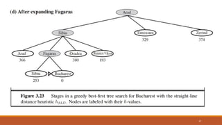
Greedy best-first search- Route finding
problems in Romania
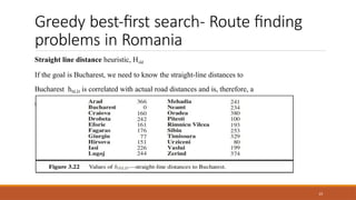
Straight line distance heuristic, Hsld
If the goal is Bucharest, we need to know the straight-line distances to
Bucharest hSLD is correlated with actual road distances and is, therefore, a
useful heuristic
23

A* search: Minimizing the total
estimated solution cost
28
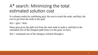
It evaluates nodes by combining g(n), the cost to reach the node, and h(n), the
cost to get from the node to the goal:
f(n) = g(n) + h(n) .
Since g(n) gives the path cost from the start node to node n, and h(n) is the
estimated cost of the cheapest path from n to the goal, we have
f(n) = estimated cost of the cheapest solution through n

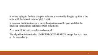
if we are trying to find the cheapest solution, a reasonable thing to try first is the
node with the lowest value of g(n) + h(n).
29
It turns out that this strategy is more than just reasonable: provided that the
heuristic function h(n) satisfies certain conditions,
A∗ search is both complete and optimal.
The algorithm is identical to UNIFORM-COST-SEARCH except that A∗ uses
g + h instead of g.

Progress of an A∗ tree search
30

Sibiu → Arad → Sibiu which would be 140+140=280
Path Traversed Distance
Arad → Sibiu 140 km
Arad → Sibiu → Fagaras 140 + 99 = 239 km
Arad → Sibiu → Rimnicu Vilcea 140 + 80 = 220 km
Arad → Sibiu → Oradea 140 + 151 = 291 km

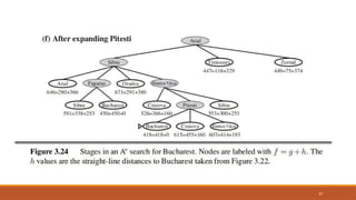
36
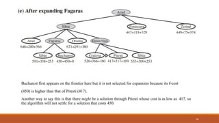
Bucharest first appears on the frontier here but it is not selected for expansion because its f-cost
(450) is higher than that of Pitesti (417).
Another way to say this is that there might be a solution through Pitesti whose cost is as low as 417, so
the algorithm will not settle for a solution that costs 450.

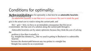
Conditions for optimality:
Admissibility
38
The first condition we require for optimality is that h(n) be an admissible heuristic.
An admissible heuristic is one that never overestimates the cost to reach the goal.
g(n) is the actual cost to reach n along the current path, and
f(n) = g(n) + h(n), we have as an immediate consequence that f(n) never
overestimates the true cost of a solution along the current path through n.
Admissible heuristics are by nature optimistic because they think the cost of solving
the
problem is less than it actually is
◦Eg, straight-line distance hSLD that we used in getting to Bucharest is n admissible
heuristic
◦because the shortest path between any two points is a straight line
◦Straight line cannot be an overestimate

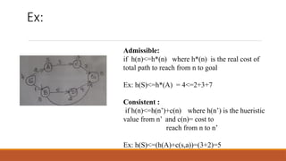
Ex:
Admissible:
if h(n)<=h*(n) where h*(n) is the real cost of
total path to reach from n to goal
Ex: h(S)<=h*(A) = 4<=2+3+7
Consistent :
if h(n)<=h(n’)+c(n) where h(n’) is the hueristic
value from n’ and c(n)= cost to
reach from n to n’
Ex: h(S)<=(h(A)+c(s,a))=(3+2)=5

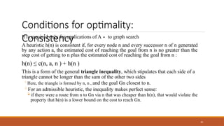
Conditions for optimality:
Consistency
40
It is required only for applications of A∗ to graph search
A heuristic h(n) is consistent if, for every node n and every successor n of n generated
by any action a, the estimated cost of reaching the goal from n is no greater than the
step cost of getting to n plus the estimated cost of reaching the goal from n :
h(n) ≤ c(n, a, n ) + h(n )
This is a form of the general triangle inequality, which stipulates that each side of a
triangle cannot be longer than the sum of the other two sides
◦Here, the triangle is formed by n, n , and the goal Gn closest to n.
◦For an admissible heuristic, the inequality makes perfect sense:
if there were a route from n to Gn via n that was cheaper than h(n), that would violate the
property that h(n) is a lower bound on the cost to reach Gn.

Optimality of
A*
41
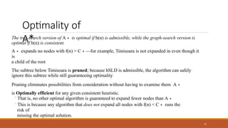
The tree-search version of A∗ is optimal if h(n) is admissible, while the graph-search version is
optimal if h(n) is consistent.
A∗ expands no nodes with f(n) > C —for
∗ example, Timisoara is not expanded in even though it
is
a child of the root
The subtree below Timisoara is pruned; because hSLD is admissible, the algorithm can safely
ignore this subtree while still guaranteeing optimality
Pruning eliminates possibilities from consideration without having to examine them A∗
is Optimally efficient for any given consistent heuristic.
◦That is, no other optimal algorithm is guaranteed to expand fewer nodes than A∗
◦This is because any algorithm that does not expand all nodes with f(n) < C∗ runs the
risk of
missing the optimal solution.

if h(n) is consistent, then the values of
f(n) along any path are nondecreasing.
42
The proof follows directly from the definition of consistency.
Suppose n is a successor of n; then g(n ) = g(n) + c(n, a, n ) for some action a, and
we have
f(n ) = g(n ) + h(n ) = g(n) + c(n, a, n ) + h(n ) g(n)
≥ + h(n) = f(n) .

whenever A∗ selects a node n for expansion,
the optimal path to that node has been
found.
43
Were this not the case, there would have to be another frontier node n on the
optimal path from the start node to n
because f is nondecreasing along any path, n would have lower f-cost than n and
would have been selected first

the sequence of nodes expanded by A∗ using GRAPH-SEARCH is
in nondecreasing order of f(n).
44
Hence, the first goal node selected for expansion must be an optimal
solution because f is the true cost for goal nodes (which have h = 0)
and all later goal nodes will be at least as expensive.

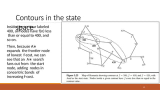
Contours in the state
space
Inside the contour labeled
400, all nodes have f(n) less
than or equal to 400, and
so on.
Then, because A∗
expands the frontier node
of lowest f-cost, we can
see that an A∗ search
fans out from the start
node, adding nodes in
concentric bands of
increasing f-cost.
45

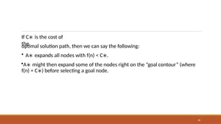
If C∗ is the cost of
the
46
optimal solution path, then we can say the following:
• A∗ expands all nodes with f(n) < C∗.
•A∗ might then expand some of the nodes right on the “goal contour” (where
f(n) = C∗) before selecting a goal node.

Disadvantages of A* Algorithm
47
The number of states within the goal contour search space is still exponential in
the length of the solution.

HEURISTIC
FUNCTIONS
•8-puzzle search space
◦Typical solution length: 20 steps
◦Average branching factor: 3
◦Exhaustive search: 320=3.5 x 109
◦Bound on unique states: 9!
= 362,880
48

Admissible Heuristics
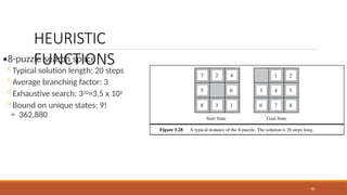
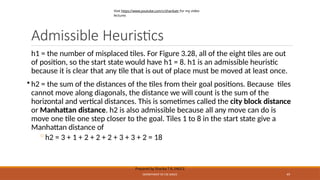
h1 = the number of misplaced tiles. For Figure 3.28, all of the eight tiles are out
of position, so the start state would have h1 = 8. h1 is an admissible heuristic
because it is clear that any tile that is out of place must be moved at least once.
• h2 = the sum of the distances of the tiles from their goal positions. Because tiles
cannot move along diagonals, the distance we will count is the sum of the
horizontal and vertical distances. This is sometimes called the city block distance
or Manhattan distance. h2 is also admissible because all any move can do is
move one tile one step closer to the goal. Tiles 1 to 8 in the start state give a
Manhattan distance of
◦h2 = 3 + 1 + 2 + 2 + 2 + 3 + 3 + 2 = 18
lectures

Heuristic Performance
Experiments on sample problems can determine the number of nodes searched and CPU time
for different strategies.
One other useful measure is effective branching factor: If a method expands N nodes to find
solution of depth d, and a uniform tree of depth d would require a branching factor of b* to
contain N nodes, the effective branching factor is b*
◦N = 1 + b* + (b*)2 + ...+ (b*)d
lectures

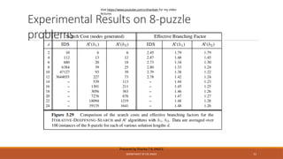
Experimental Results on 8-puzzle
problems
lectures

Quality of
Heuristics
Since A* expands all nodes whose f value is less than that of an optimal solution, it is always
better to use a heuristic with a higher value as long as it does not over-estimate.
Therefore h2 is uniformly better than h1 , or h2 dominates h1 .
A heuristic should also be easy to compute, otherwise the overhead of computing the heuristic
could outweigh the time saved by reducing search (e.g. using full breadth-first search to
estimate distance wouldn’t help)
lectures

Inventing Heuristics
Many good heuristics can be invented by considering relaxed versions of the problem
(abstractions).
For 8-puzzle: A tile can move from square A to B if A is adjacent to B and B is blank
◦(a) A tile can move from square A to B if A is adjacent to B.
◦(b) A tile can move from square A to B if B is blank. (c) A tile can move from square A to B.
If there are a number of features that indicate a promising or unpromising state, a weighted sum
of these features can be useful. Learning methods can be used to set weights.
lectures

Memory-bounded heuristic search
Algorithms
1. Iterative-deepening A (IDA*)
∗
2. Recursive best-first search (RBFS)
3. Simplified Memory bounded A* (SMA*)

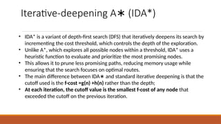
Iterative-deepening A (IDA*)
∗
• IDA* is a variant of depth-first search (DFS) that iteratively deepens its search by
incrementing the cost threshold, which controls the depth of the exploration.
• Unlike A*, which explores all possible nodes within a threshold, IDA* uses a
heuristic function to evaluate and prioritize the most promising nodes.
• This allows it to prune less promising paths, reducing memory usage while
ensuring that the search focuses on optimal routes.
• The main difference between IDA and standard iterative deepening is that the
∗
cutoff used is the f-cost =g(n) +h(n) rather than the depth;
• At each iteration, the cutoff value is the smallest f-cost of any node that
exceeded the cutoff on the previous iteration.

Recursive best-first search (RBFS)

Simplified Memory bounded A* (SMA*)
• SMA proceeds just like A , expanding the best leaf until memory is full.
∗ ∗
• At this point, it cannot add a new node to the search tree without
dropping an old one.
• SMA always drops the worst leaf node—the one with the highest f-value.
∗
Like RBFS, SMA then backs up the value of the forgotten node to its
∗
parent.
• In this way, the ancestor of a forgotten subtree knows the quality of the
best path in that subtree.
• With this information, SMA regenerates the subtree only when all other
∗
paths have been shown to look worse than the path it has forgotten.

4.Module_2_Chaptjvyfgcgfxfdxhgfxchtfer_3.pptx

More Related Content

Similar to 4.Module_2_Chaptjvyfgcgfxfdxhgfxchtfer_3.pptx

Recently uploaded

4.Module_2_Chaptjvyfgcgfxfdxhgfxchtfer_3.pptx