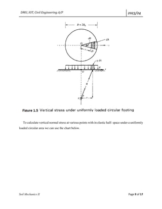
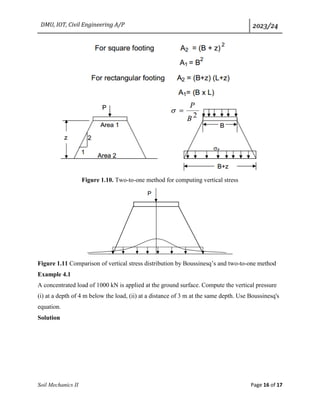
This document discusses the estimation of vertical stresses in soil masses due to external loads, emphasizing the application of elasticity theory for predicting settlements of structures. It outlines key formulas, such as Boussinesq's and Westergaard's, for computing stresses from point, line, and strip loads, while acknowledging the real-world variations in soil properties. Various methods for solving stress distribution problems, including equivalent point load method and Newmark's influence charts, are described to aid in practical applications for geotechnical engineering.

![DMU, IOT, Civil Engineering A/P 2023/24
Soil Mechanics II Page 11 of 17
acting as a concentrated load through its center of gravity. Then radial distances of CG’s of this
small units from the vertical axis passing through the point at which stress is to be calculated are
computed (r1, r2, r3,..). Then for various 𝑟1 𝑧
⁄ , 𝑟2 𝑧
⁄ , 𝑟3 𝑧
⁄ ...corresponding 𝐼𝐵1, 𝐼𝐵2, 𝐼𝐵3,...are
obtained from ready rocken. The vertical normal stress 𝜎𝑧 is given as
𝜎𝑧 =( 𝑄1 𝑧2
⁄ )( 𝐼𝐵1) + (𝑄2 𝑧2
⁄ )(𝐼𝐵2) + (𝑄3 𝑧2
⁄ )(𝐼𝐵3) + (𝑄4 𝑧2
⁄ )(𝐼𝐵4)
=(1 𝑧2
⁄ ){𝑄1𝐼𝐵1 + 𝑄2𝐼𝐵2+𝑄3𝐼𝐵3 + ⋯ }
Where 𝑄1, 𝑄2, 𝑄3, are equivalent concentrated loads acting through unit area 1,2,3,... and 𝑄1
= 𝑄𝐴1, 𝑄2 = 𝑄𝐴2, 𝑄3 = 𝑄𝐴3...where Q is the uniformly distributed load over entire area and 𝐴1,
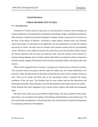
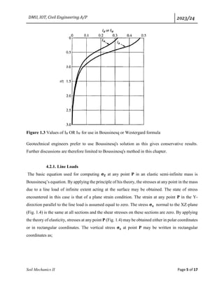
𝐴2, 𝐴3,...are areas of small unit areas 1,2,3...respectively. For example if the normal stress at a
depth z below the center of rectangular footing, of dimension L & B Shown in fig.1.7, is to be
computed, then we proceed as follows
Figure 1.7 Q units/ unit area
𝑟1 = √[
𝐿
4
]2 + [
𝐵
4
]2
Q1=Q2=Q3=Q4=Q4=Q (L/2) (B/2)
Calculate 0.3z. Then divide whole area in to smaller units of dimensions less than 0.3z. let in this
example L/2 AND B/2<0.3z, then we can divide the rectangle in to four smaller units of
dimensions L/2*B/2 as shown in fig. computation of A1, A2, A2, A4 and Q1, Q2, Q3 and Q4 and](https://image.slidesharecdn.com/4-241220072806-e3870fd1/85/4-Chapter-FOUR-Stres-ses-In-Soils-pdf-11-320.jpg)
![DMU, IOT, Civil Engineering A/P 2023/24
Soil Mechanics II Page 12 of 17
r1, r2, r3 and r4 are shown in fig knowing r1/z, r2/z, r3/z and r4/z Boussinesq’s influence factor
𝐼𝐵1, 𝐼𝐵2,𝐼𝐵3 , and 𝐼𝐵4 are obtained from ready reckon or calculated using the equation
Then 𝜎𝑍 at pint ‘A’ at a depth ‘z’ on the line passing through center of the shown area is
𝜎𝑍=(Q1/z2
)(𝐼𝐵1)+(Q2/z2
)( 𝐼𝐵2)+(Q3/z2
)+( 𝐼𝐵3)+ (Q4/z2
)( 𝐼𝐵4)
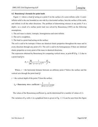
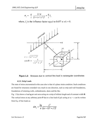
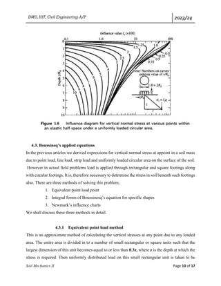
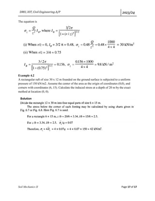
4.3.2 Integral forms of Boussinesq’s equation for specific shapes
For rectangular load areas, which are the common form of footing loads, in actual field,
Boussineq’s equation for point loads has been integrated by Prof. Fadum. The solution
obtained is little difficult mathematically and it is usually used with the help of charts.
The mathematical solution as obtained for comparing at a corner of a rectangular footing of
dimensions mz and nz at a depth z carrying a uniform load intensity q units/unit area can be
written in the form
𝝈𝒁=q𝑰𝑹
Where IR is another influence factor and is given by
IR =
1
4
[
2mn(m2+n2+1)
1 2
⁄
m2+n2+m2n2+1
m2+n2+2
m2+n2+1
+ tan−1 2mn(m2+n2+1)
1 2
⁄
m2+n2−m2n2+1
]
Values of IR for different values of log m and different values of n are plotted in the figure
given below. The values of IR can be easily read from the graph and hence 𝝈𝒁 can be
effortlessly calculated for this particular type of problems.](https://image.slidesharecdn.com/4-241220072806-e3870fd1/85/4-Chapter-FOUR-Stres-ses-In-Soils-pdf-12-320.jpg)
![DMU, IOT, Civil Engineering A/P 2023/24
Soil Mechanics II Page 13 of 17
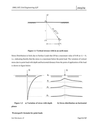
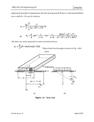
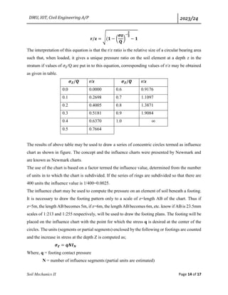
4.3.3 Newmark’s Influence Charts
We know that for a circularly loaded area of radius r the value at a point at a depth z vertical
line passing through center of loaded area is given by
𝝈𝒁=q[𝟏 − {
𝟏
𝟏+(𝑹/𝒛)𝟐
}
𝟑/𝟐
]
If we rearrange this equation and solve for r/z and take the positive root we get](https://image.slidesharecdn.com/4-241220072806-e3870fd1/85/4-Chapter-FOUR-Stres-ses-In-Soils-pdf-13-320.jpg)


![Geotechnical Engineering-II [Lec #6: Stress Distribution in Soil]](https://cdn.slidesharecdn.com/ss_thumbnails/6-180930132732-thumbnail.jpg?width=640&height=640&fit=bounds)


![Geotechnical Engineering-II [Lec #7: Soil Stresses due to External Load]](https://cdn.slidesharecdn.com/ss_thumbnails/7-180930132739-thumbnail.jpg?width=640&height=640&fit=bounds)
![Geotechnical Engineering-II [Lec #9+10: Westergaard Theory]](https://cdn.slidesharecdn.com/ss_thumbnails/9-181020124827-thumbnail.jpg?width=640&height=640&fit=bounds)
![Geotechnical Engineering-II [Lec #7A: Boussinesq Method]](https://cdn.slidesharecdn.com/ss_thumbnails/7a-181020124807-thumbnail.jpg?width=640&height=640&fit=bounds)


