Divide-and-Conquer Design
Paradigm
Thedivide-and-conquer method is a powerful strategy for
designing asymptotically efficient algorithms.
The divide-and-conquer design paradigm:
Divide the problem (instance) into one or more subproblems.
Conquer the subproblems by solving them recursively.
Combine subproblem solutions to form a solution to the original
problem.
4.
Merge Sort
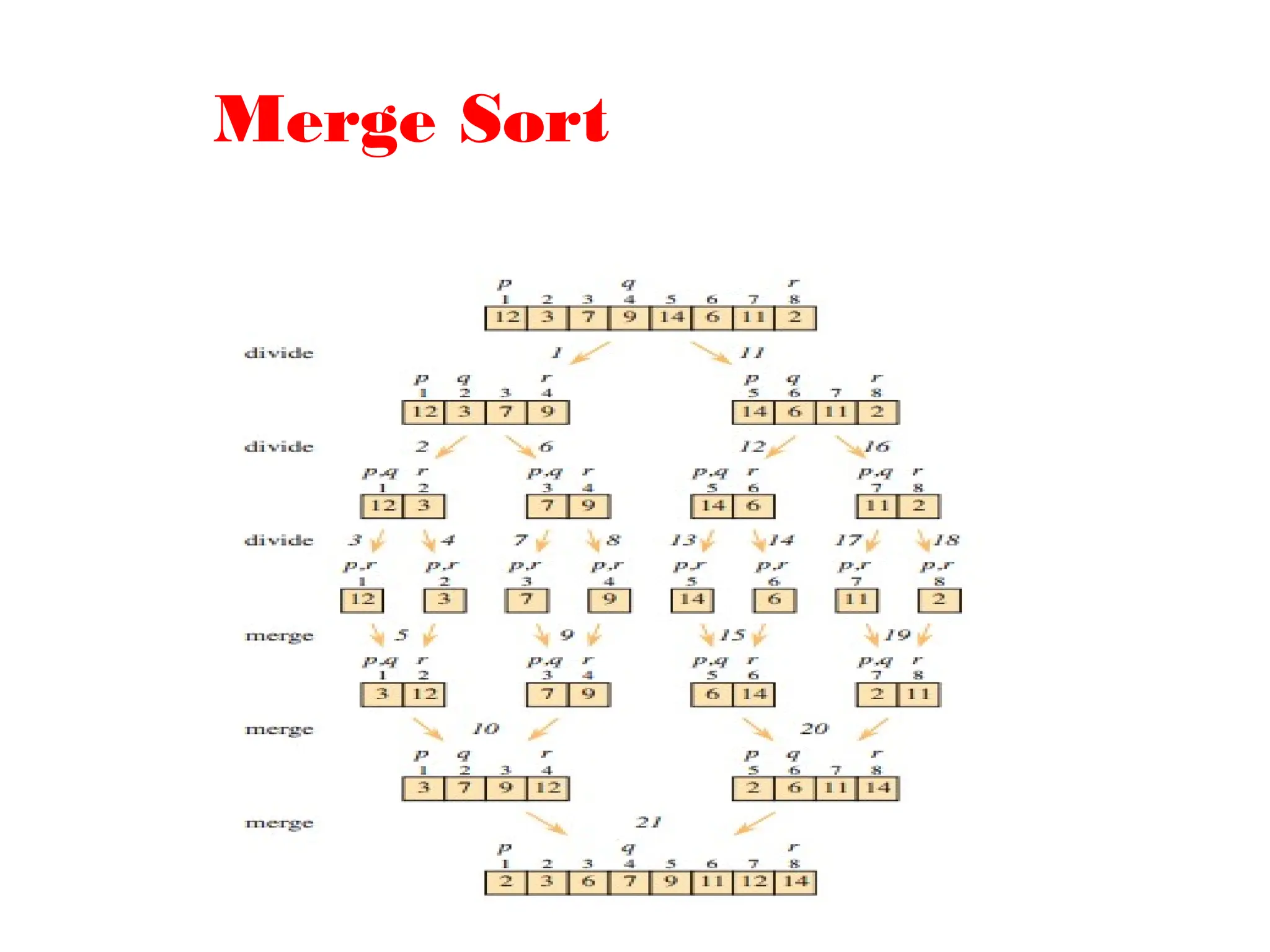
Dividethe subarray A[p:r] to be sorted into two adjacent
subarrays, each of half the size.
To do so, compute the midpoint q of A[p:r] (taking the average of
p and r), and divide A[p: r] into subarrays A[p:q] and A[q+1: r].
Conquer by sorting each of the two subarrays A[p:q] and
A[q+1:r] recursively using merge sort.
Combine by merging the two sorted subarrays A[p:q] and
A[q+1:r] back into A[p:r], producing the sorted answer.
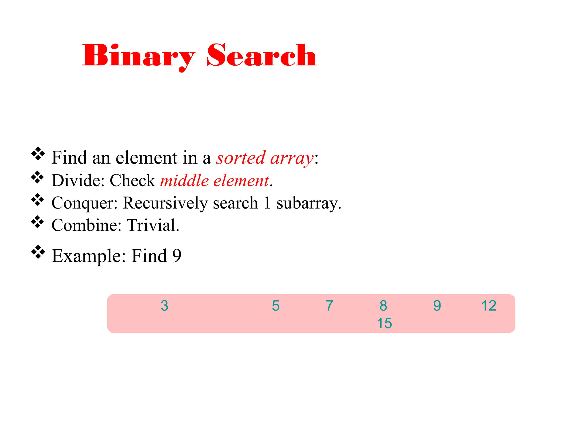
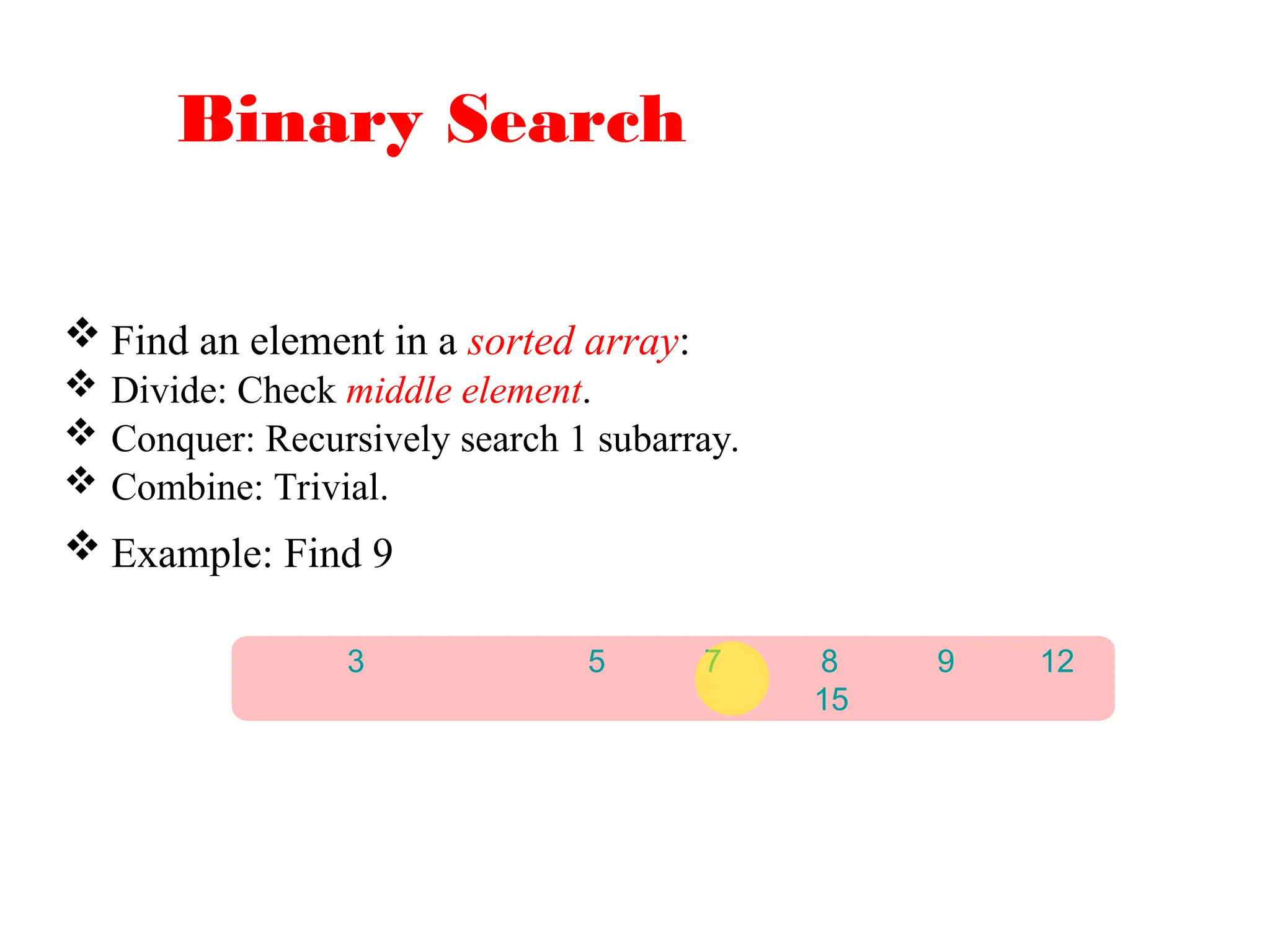
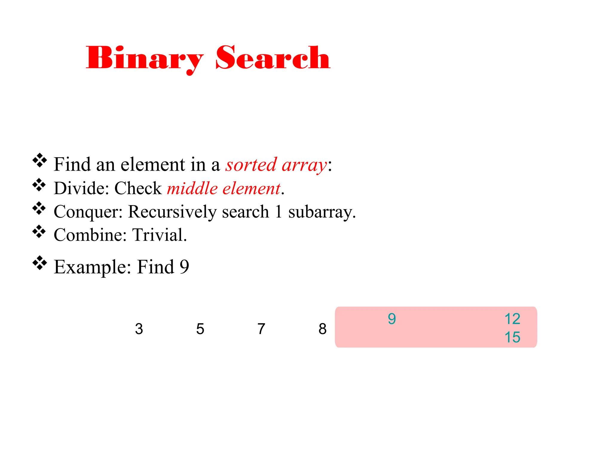
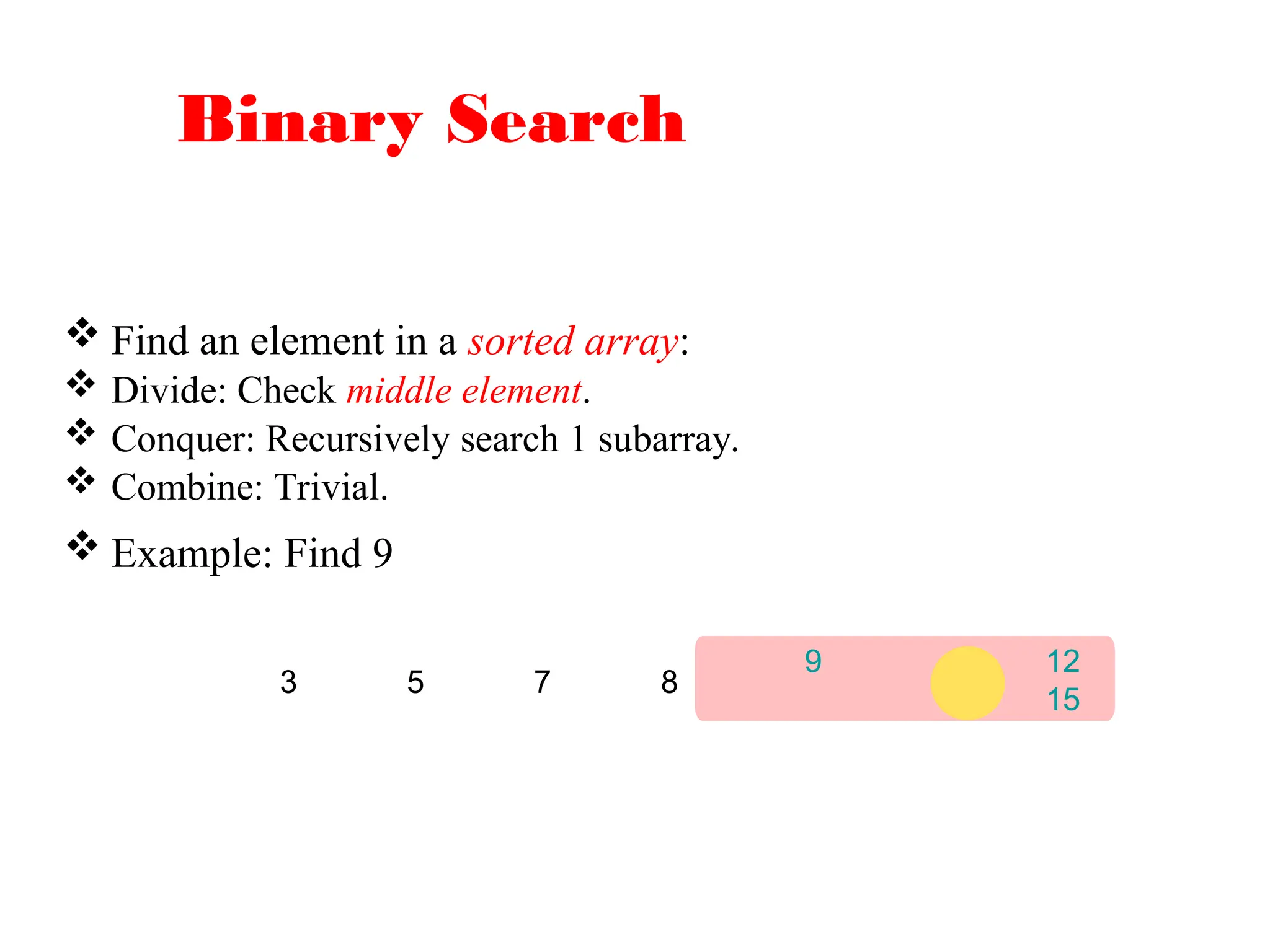
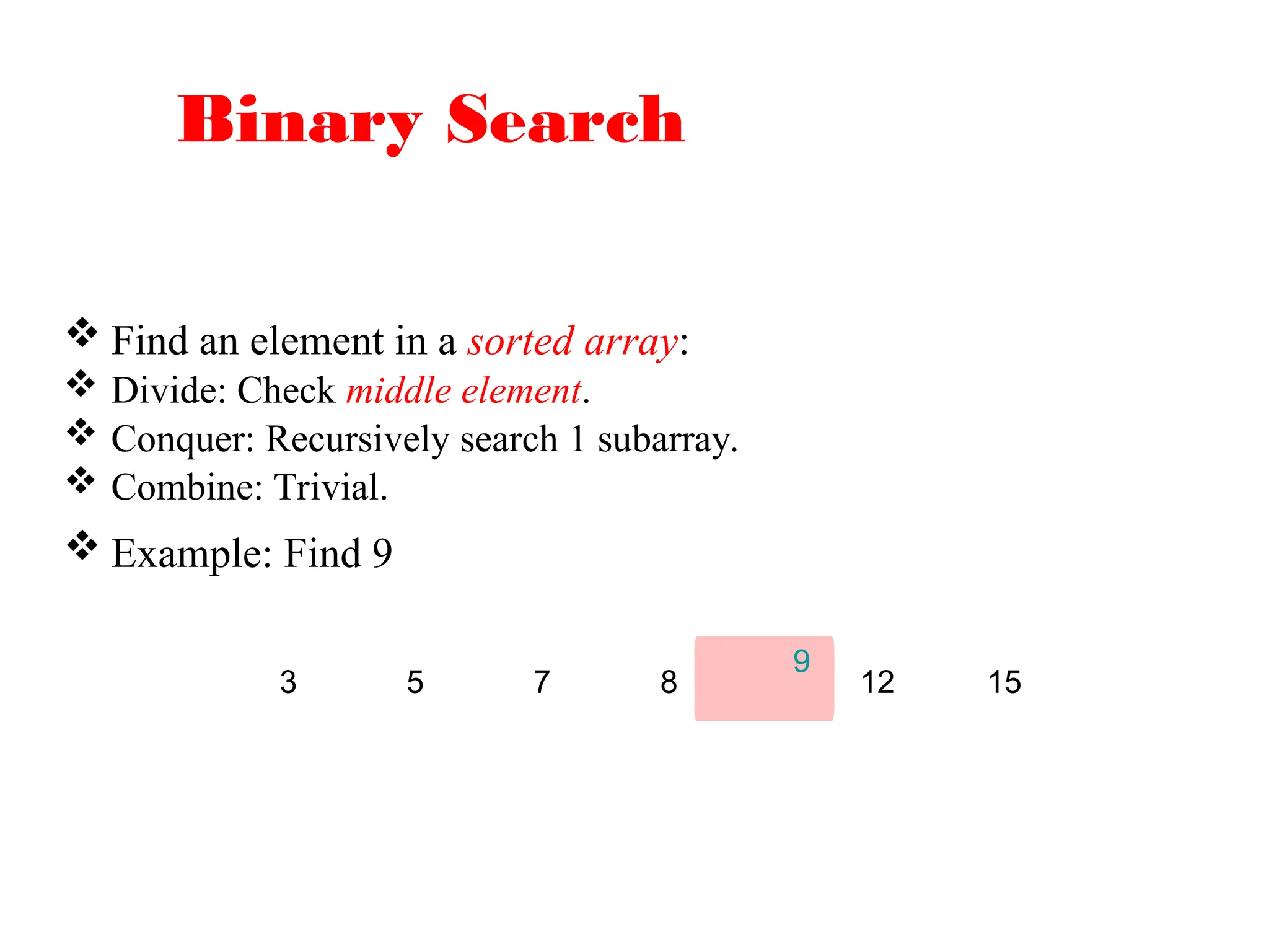
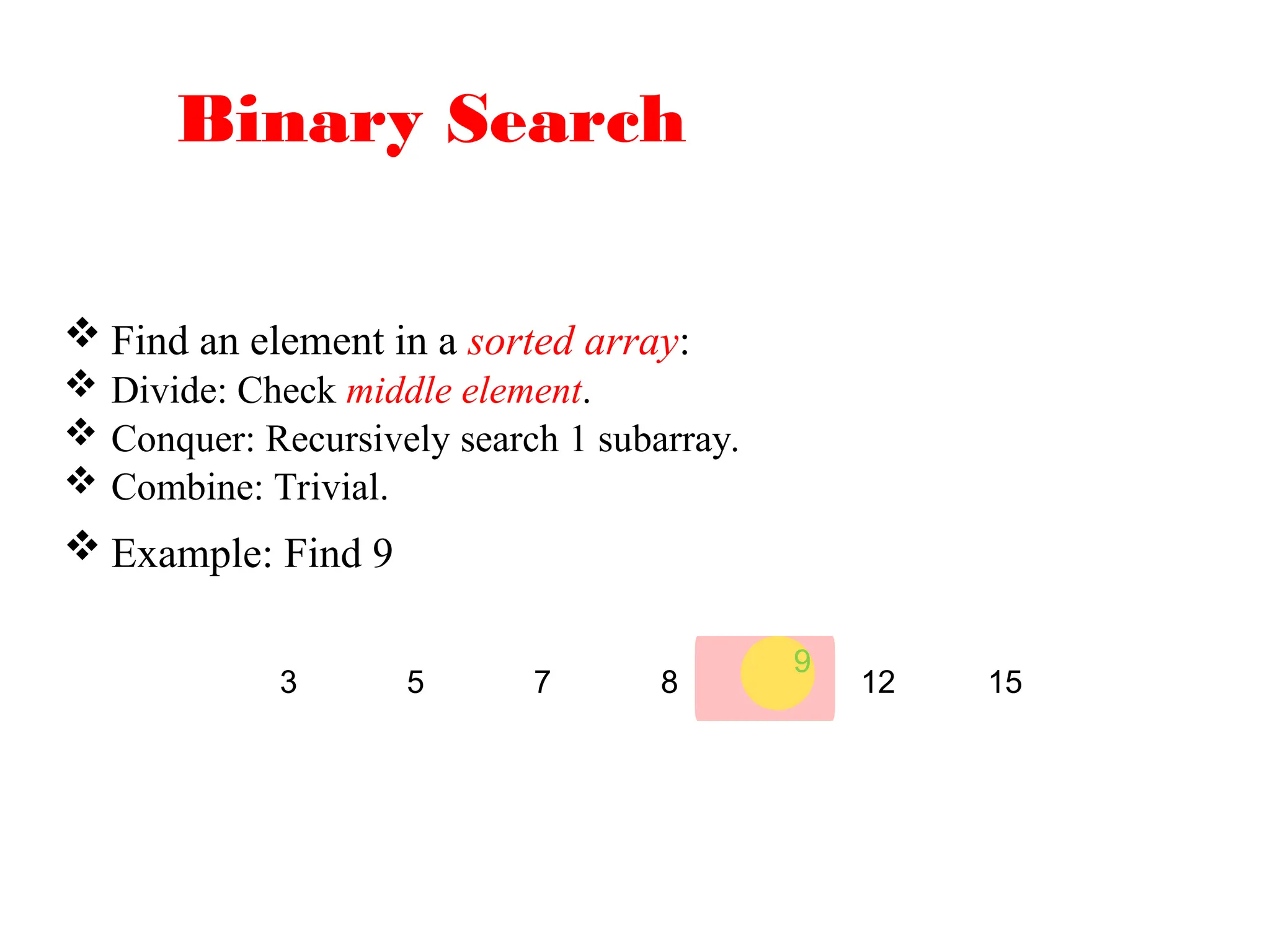
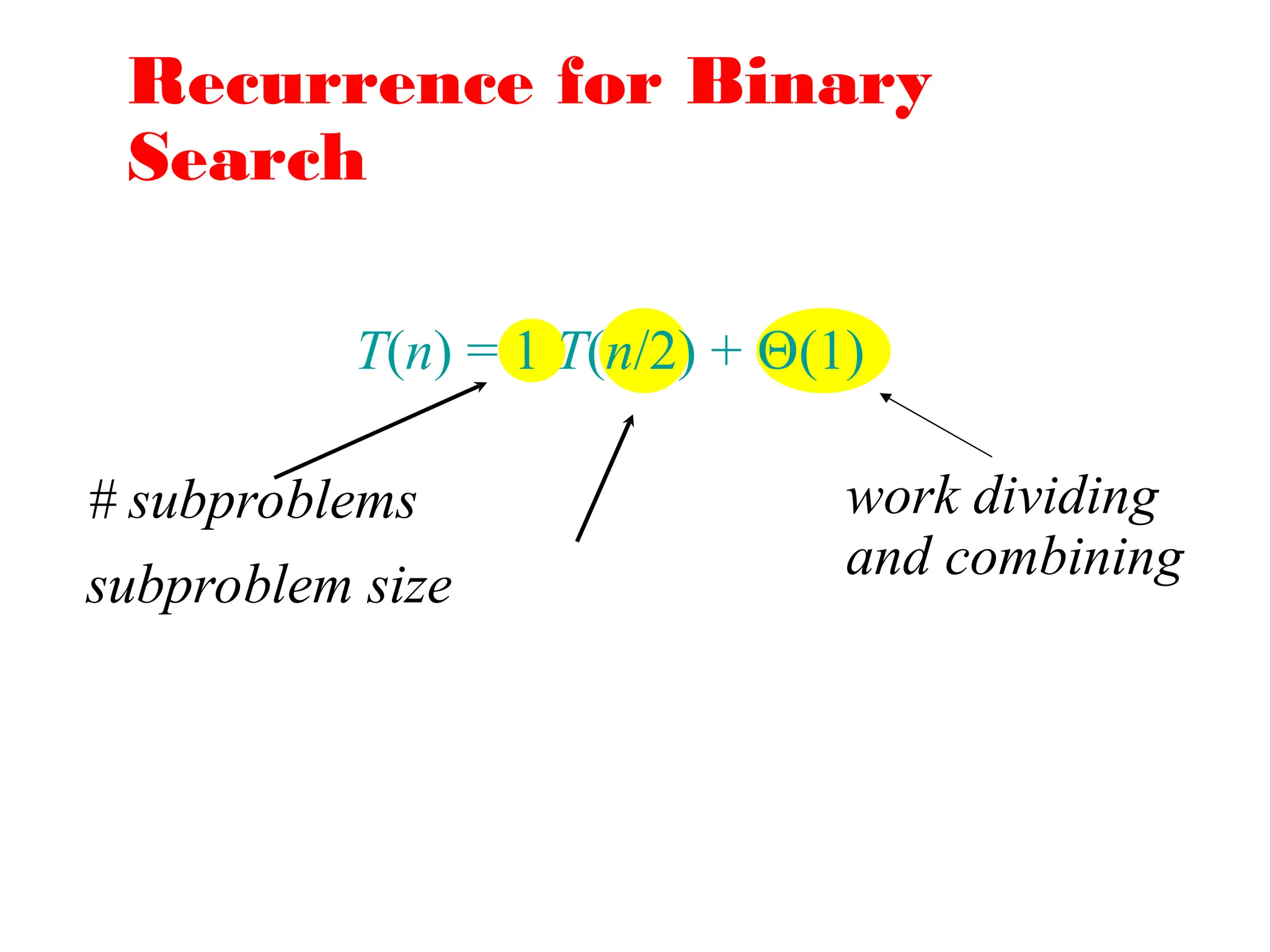
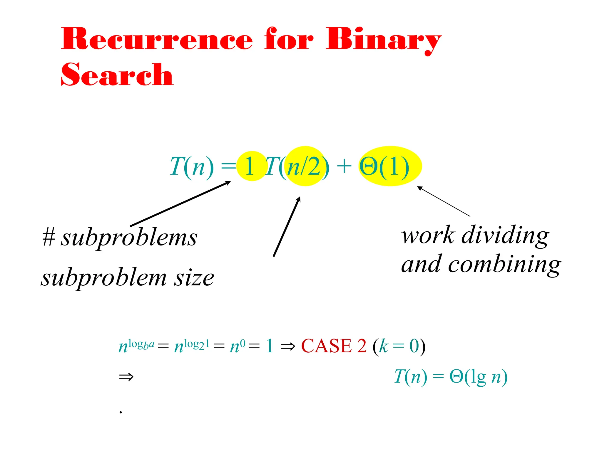
Recurrence for Binary
Search
T(n)= 1 T(n/2) + (1)
# subproblems
subproblem size
work dividing
and combining
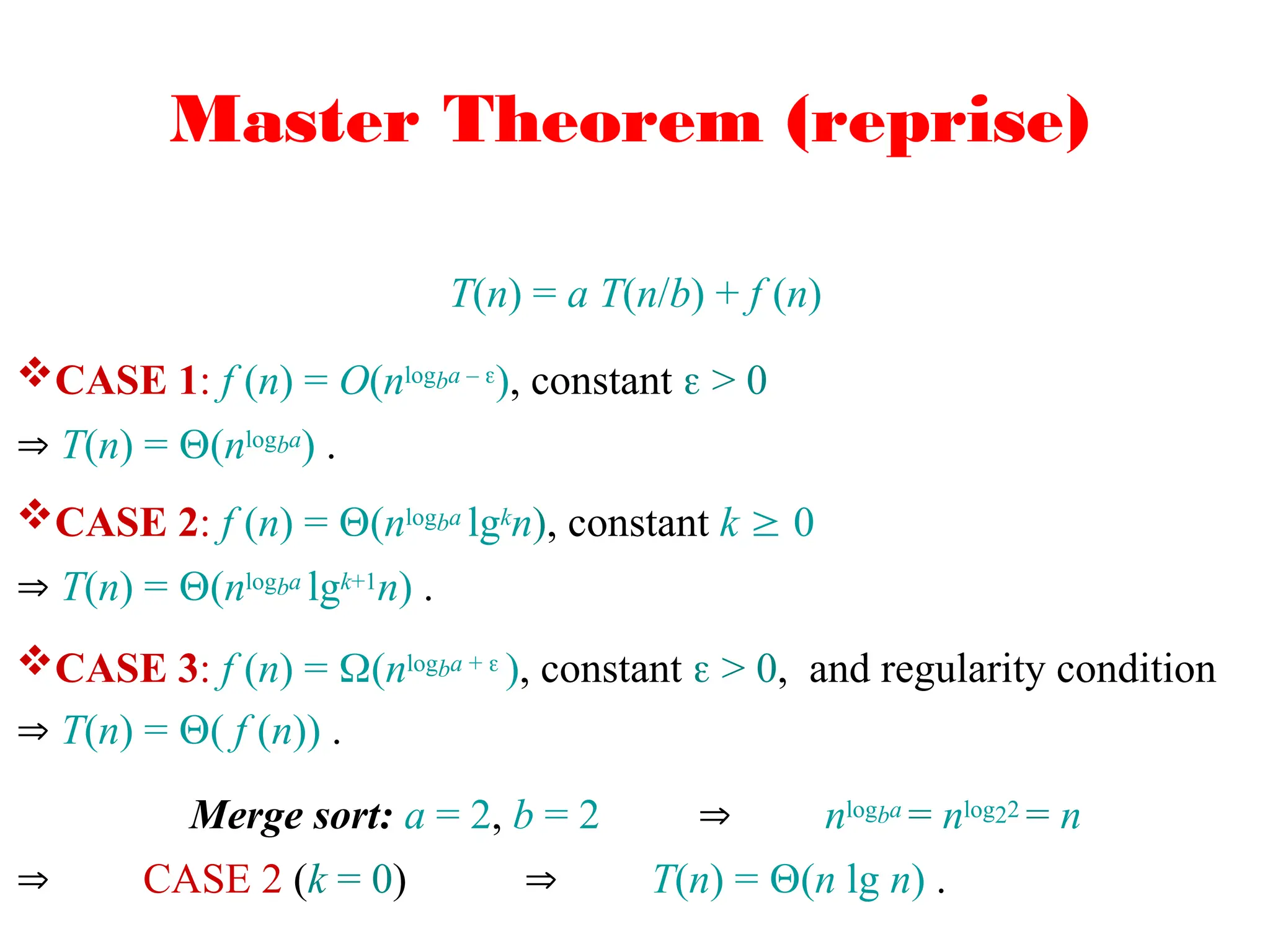
nlogba = nlog21 = n0 = 1 CASE 2 (k = 0)
T(n) = (lg n)
.
18.
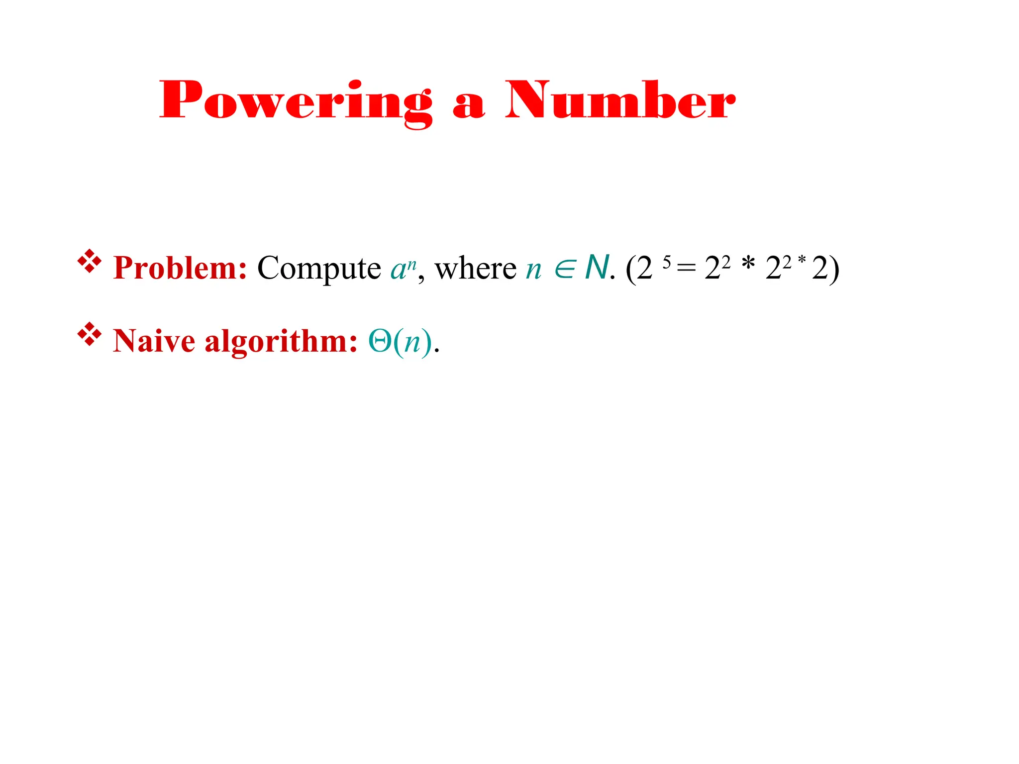
Powering a Number
Problem: Compute an, where n N. (2 5
= 22
* 22 *
2)
Naive algorithm: (n).
19.
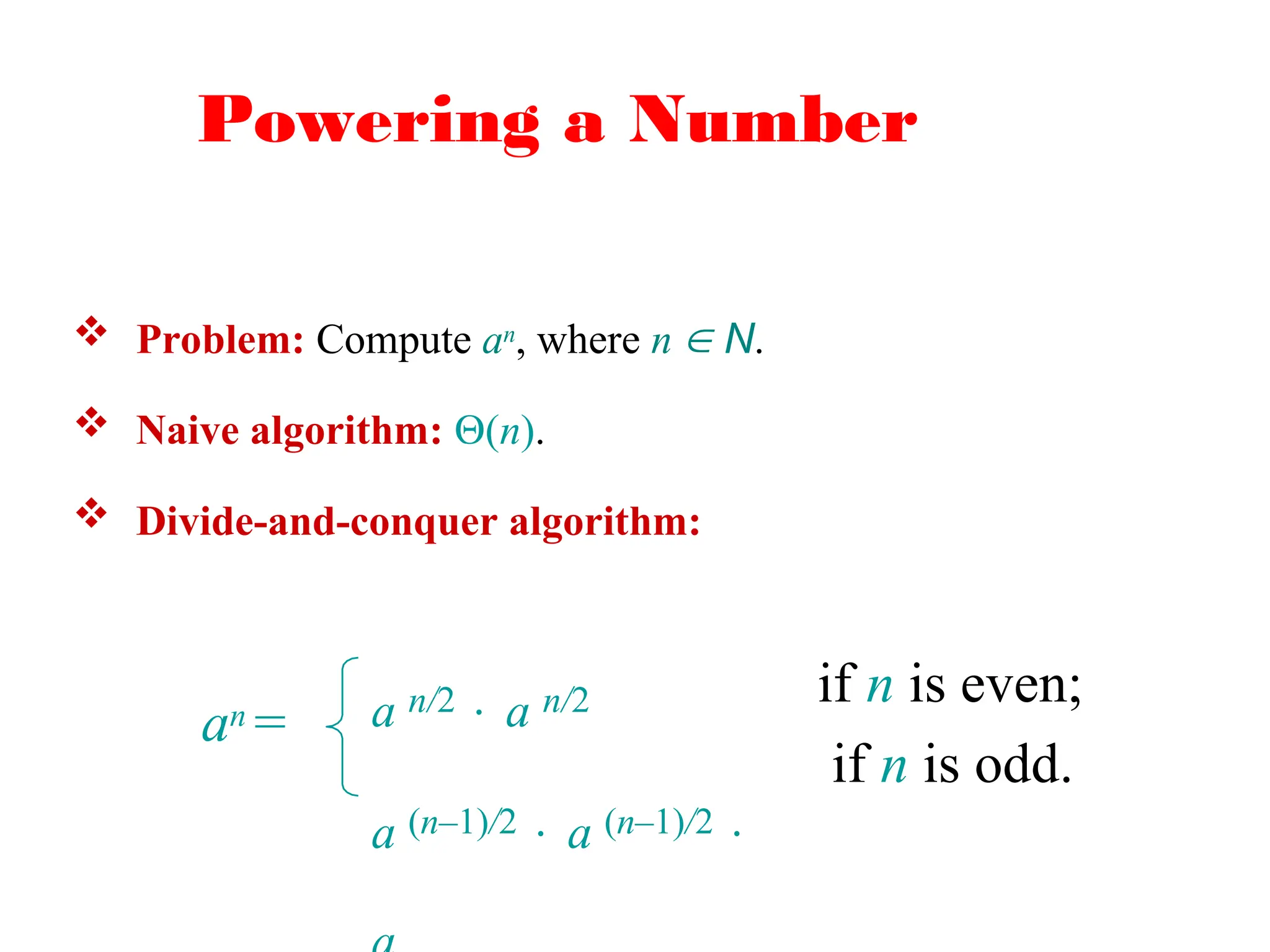
Powering a Number
an= a n/2 a n/2
a (n–1)/2 a (n–1)/2
if n is even;
if n is odd.
Problem: Compute an, where n N.
Naive algorithm: (n).
Divide-and-conquer algorithm:
20.
Powering a Number
an= a n/2 a n/2
a (n–1)/2 a (n–1)/2
a
if n is even;
if n is odd.
Problem: Compute an, where n N.
Naive algorithm: (n).
Divide-and-conquer algorithm:
T(n) = T(n/2) + (1) T(n) = (lg n) .
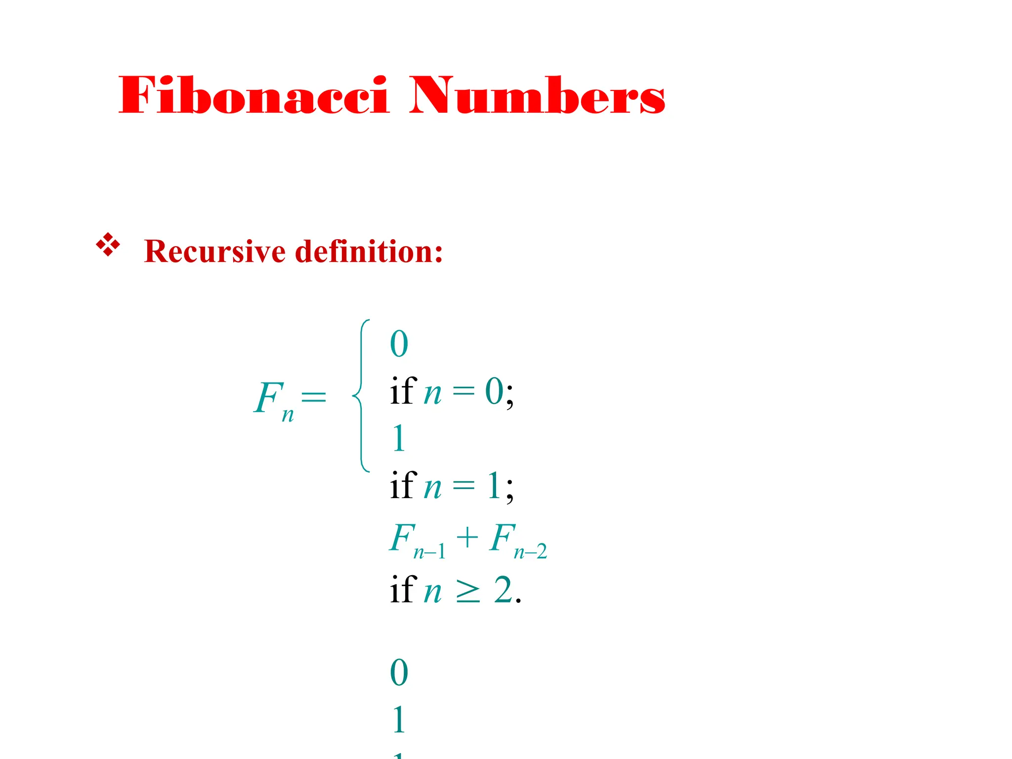
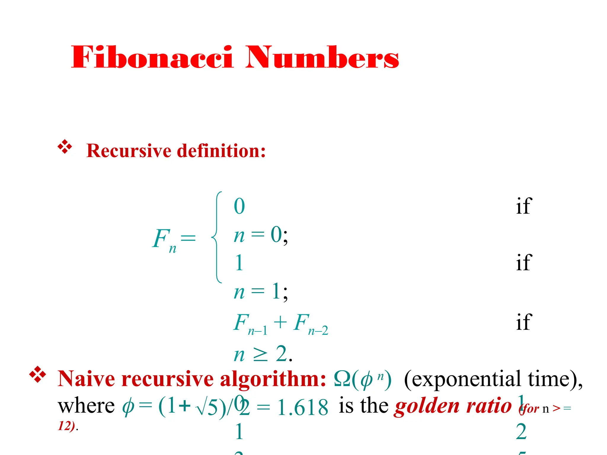
Fibonacci Numbers
Recursivedefinition:
Fn =
0 if
n = 0;
1 if
n = 1;
Fn–1 + Fn–2 if
n 2.
0 1
1 2
Naive recursive algorithm: ( n) (exponential time),
where = (1 is the golden ratio (for n > =
12).
5)/ 2 = 1.618
Computing Fibonacci
Numbers
Bottom-up:
Compute F0, F1, F2, …, Fn in order, forming each number
by summing the two previous.
Running time: (n).
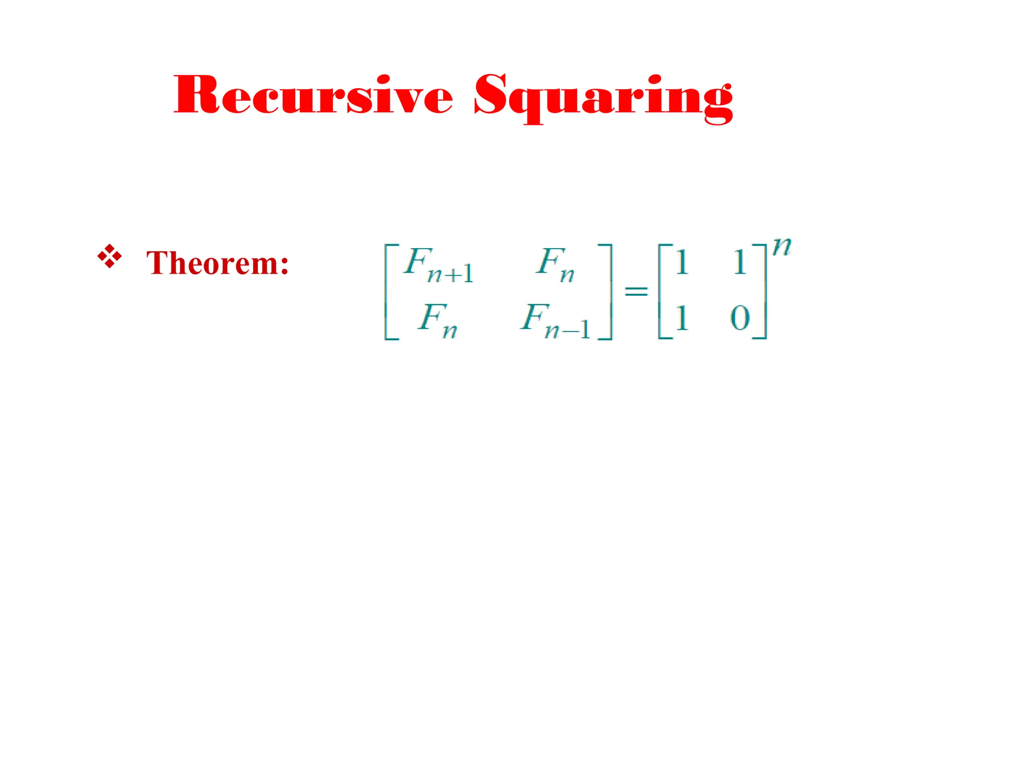
Naive recursive squaring:
Fn = n/ 5 rounded to the nearest integer.
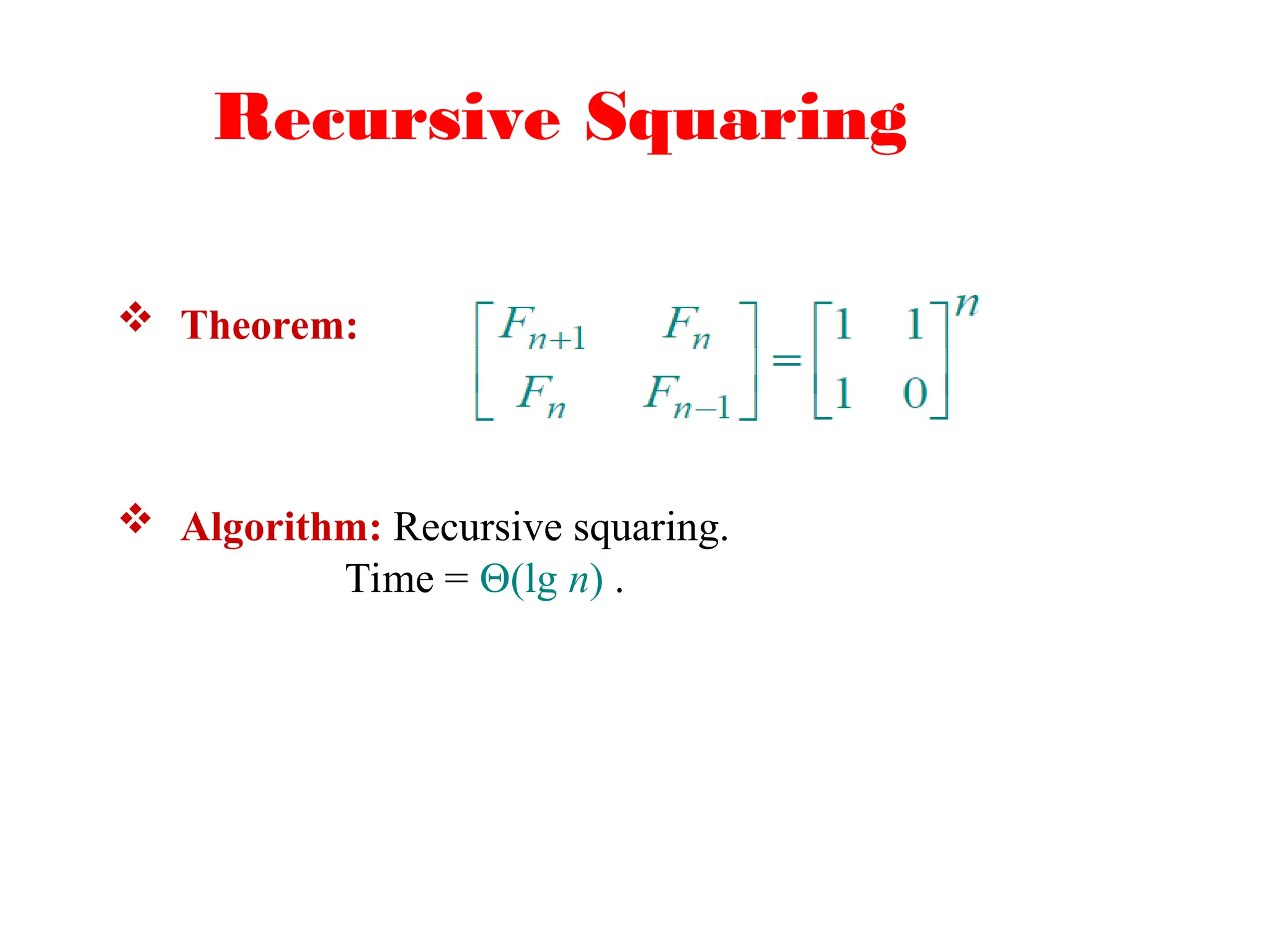
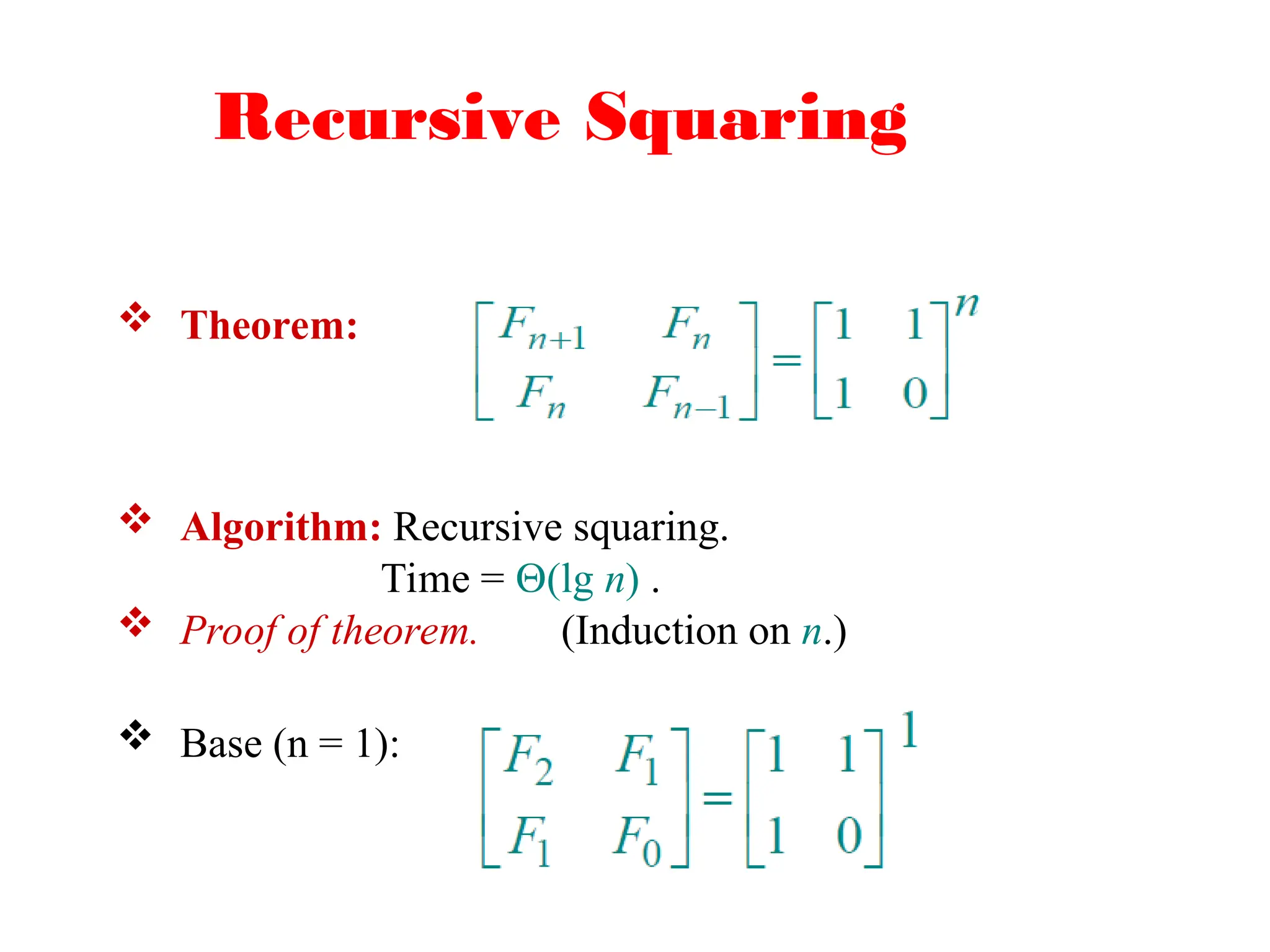
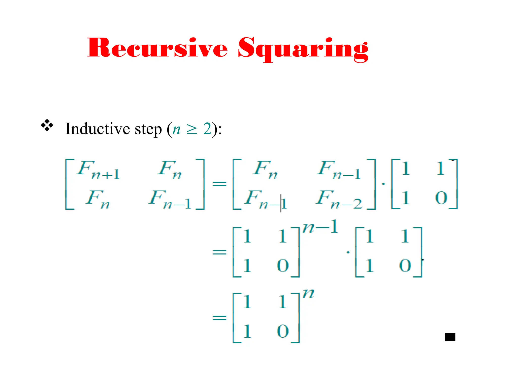
Recursive squaring: (lg n) time.
This method is unreliable, since floating-point arithmetic is
prone to round-off errors.
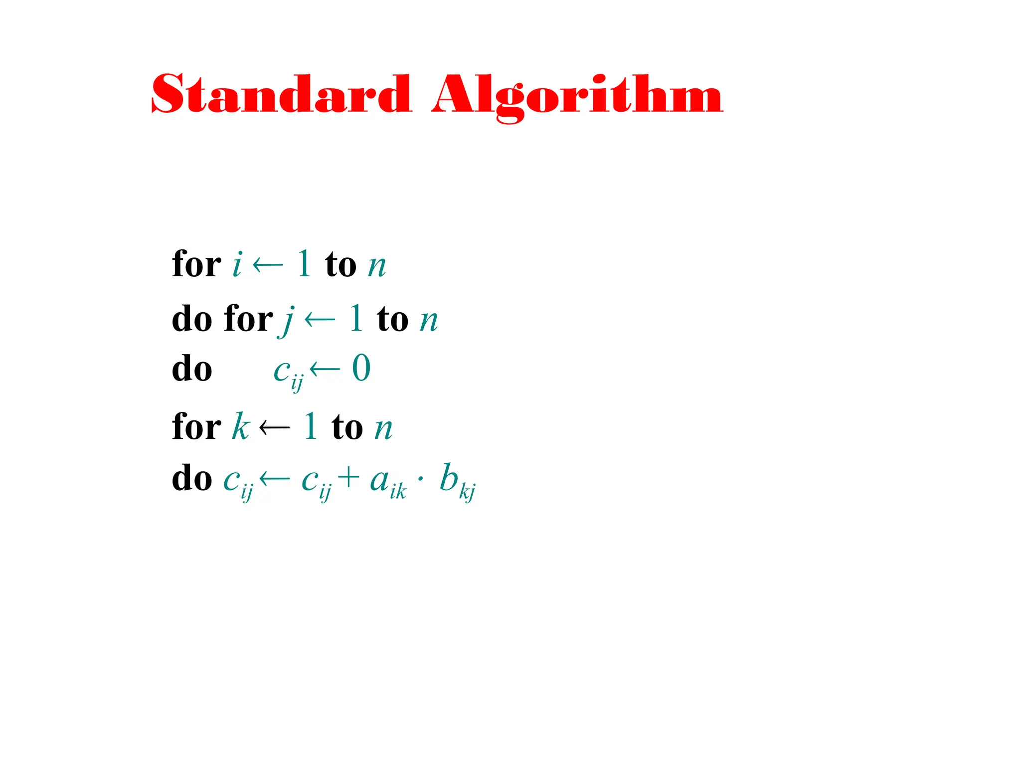
Standard Algorithm
for i 1 to n
do for j 1 to n
do cij 0
for k 1 to n
do cij cij + aik bkj
31.
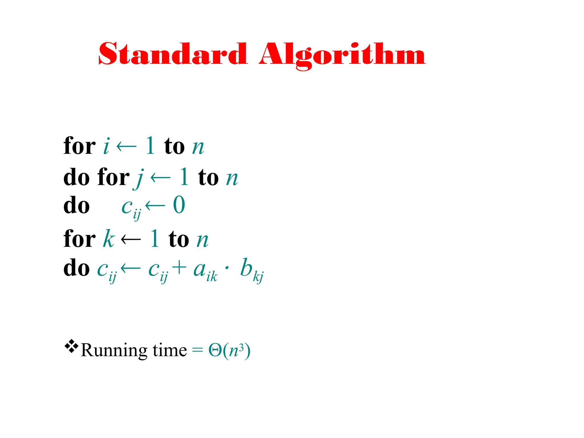
Standard Algorithm
for i 1 to n
do for j 1 to n
do cij 0
for k 1 to n
do cij cij + aik bkj
Running time = (n3)
32.
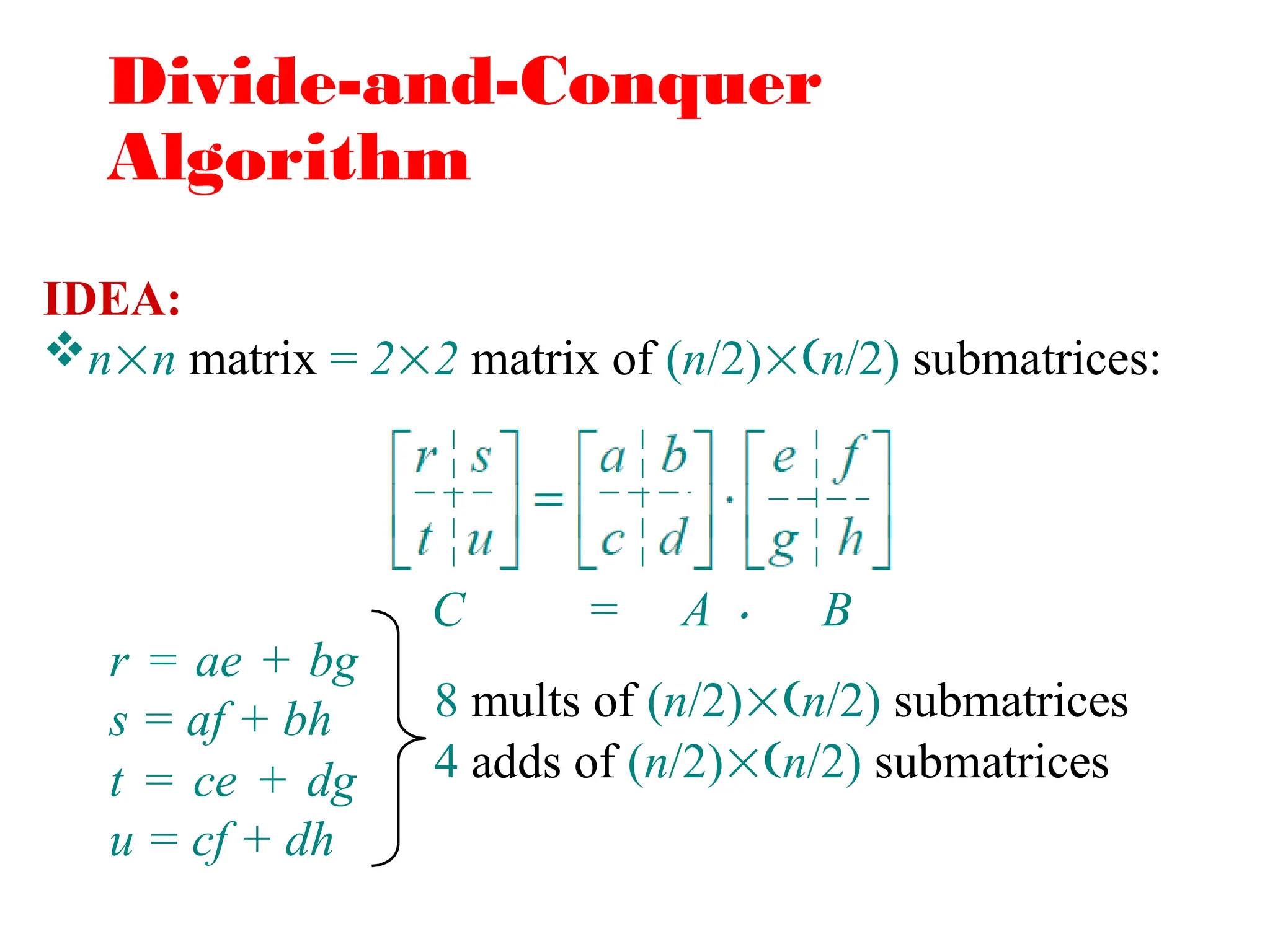
Divide-and-Conquer
Algorithm
IDEA:
nn matrix =22 matrix of (n/2)n/2) submatrices:
C = A
r = ae + bg
s = af + bh
t = ce + dg
u = cf + dh
8 mults of (n/2)n/2) submatrices
4 adds of (n/2)n/2) submatrices
B
33.
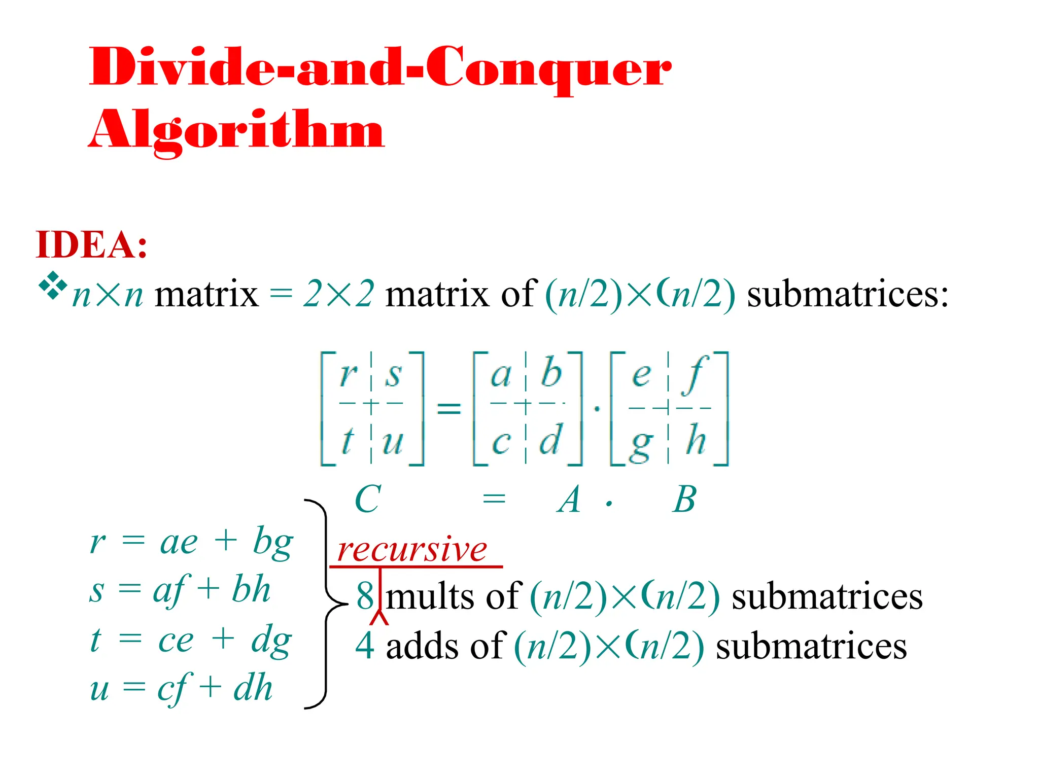
Divide-and-Conquer
Algorithm
IDEA:
nn matrix =22 matrix of (n/2)n/2) submatrices:
C = A
r = ae + bg
s = af + bh
t = ce + dg
u = cf + dh
8 mults of (n/2)n/2) submatrices
4 adds of (n/2)n/2) submatrices
B
^
recursive
34.
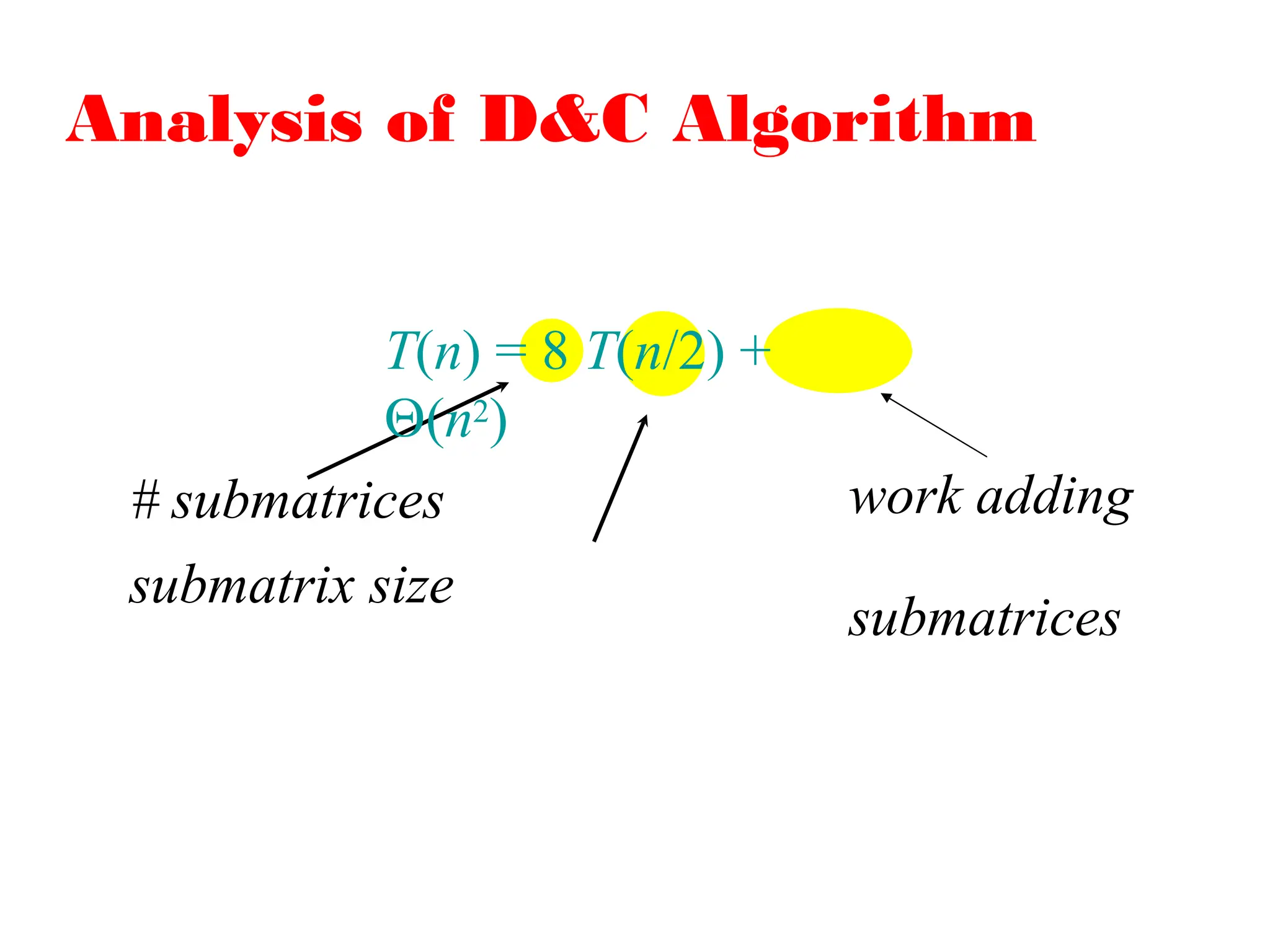
Analysis of D&CAlgorithm
# submatrices
submatrix size
work adding
submatrices
T(n) = 8 T(n/2) +
(n2)
35.
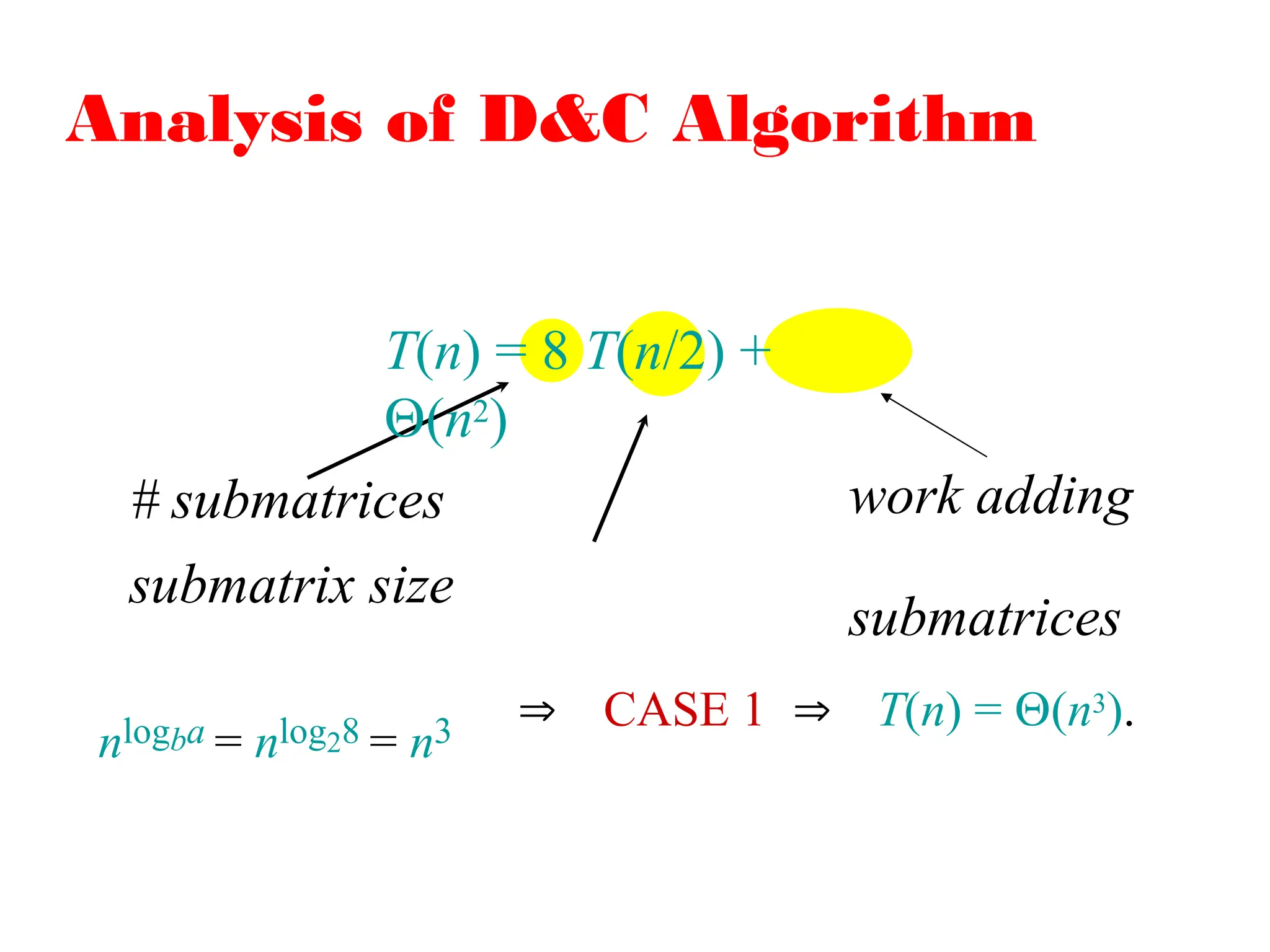
Analysis of D&CAlgorithm
# submatrices
submatrix size
work adding
submatrices
T(n) = 8 T(n/2) +
(n2)
nlogba = nlog28 = n3 CASE 1 T(n) = (n3).
36.
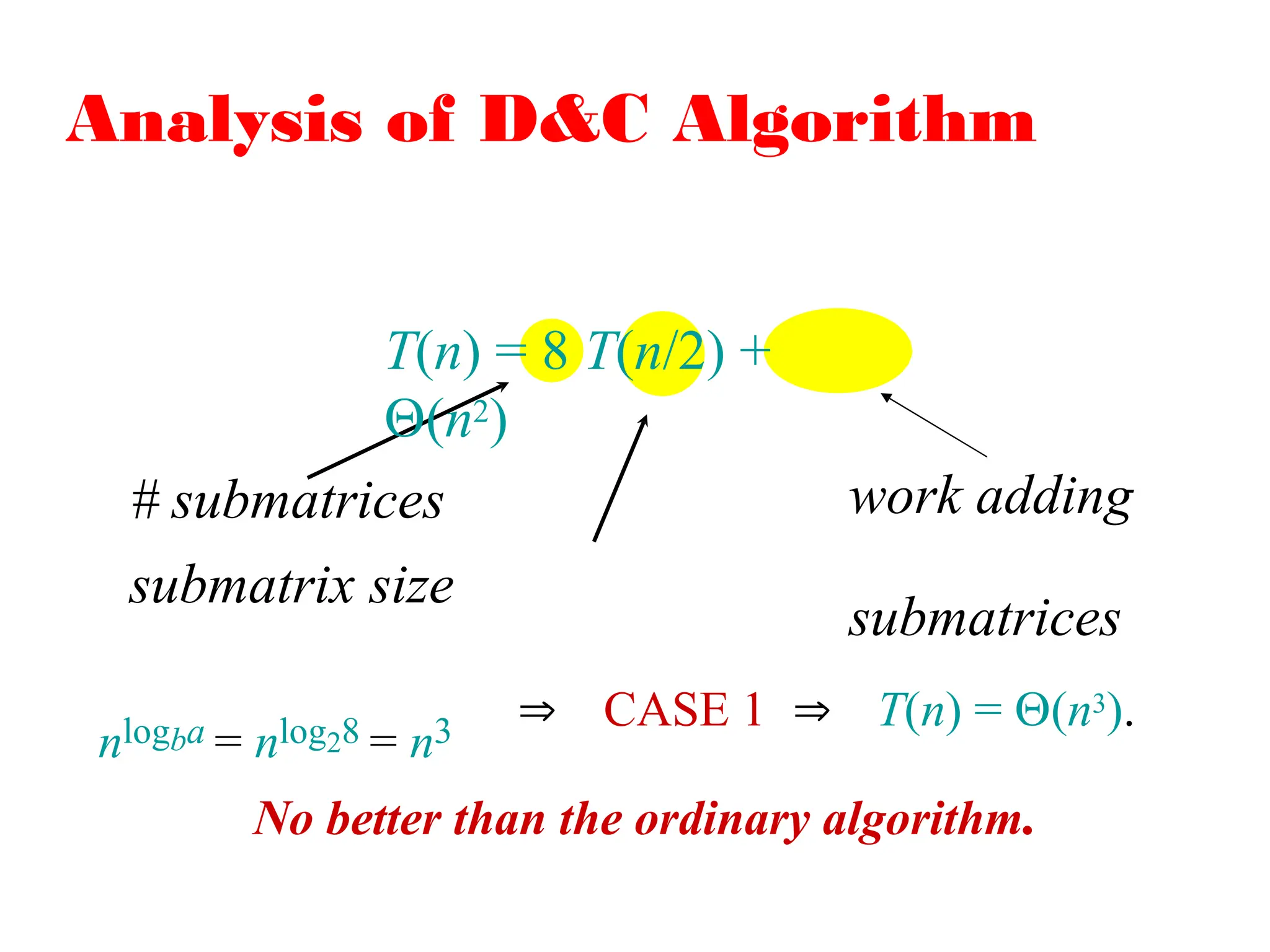
Analysis of D&CAlgorithm
# submatrices
submatrix size
work adding
submatrices
T(n) = 8 T(n/2) +
(n2)
nlogba = nlog28 = n3 CASE 1 T(n) = (n3).
No better than the ordinary algorithm.
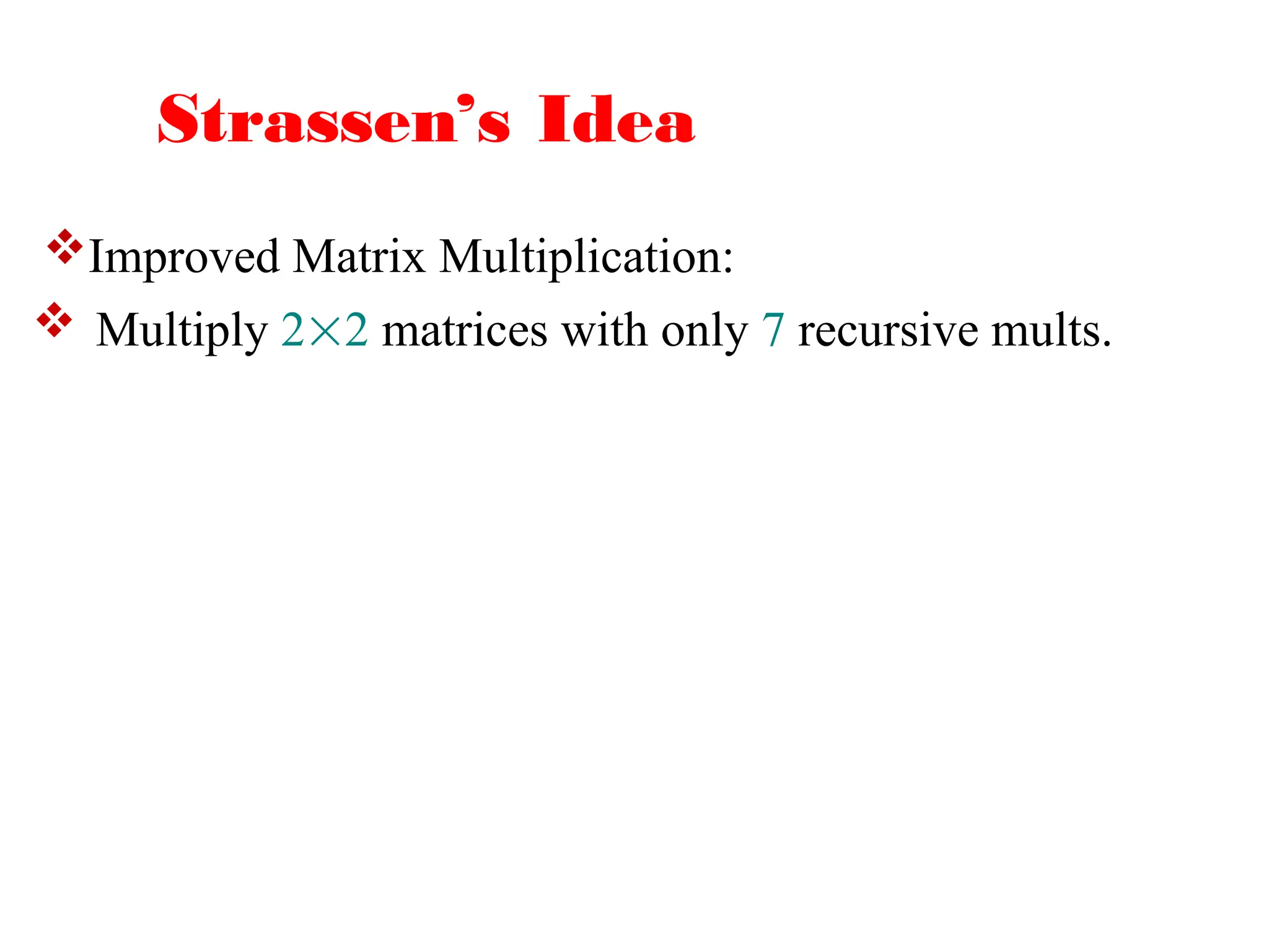
Strassen’s Idea
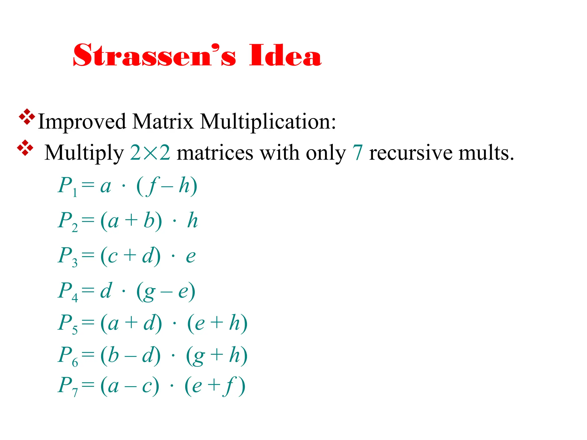
Multiply22 matrices with only 7 recursive mults.
P1 = a ( f – h)
P2 = (a + b) h
P3 = (c + d) e
P4 = d (g – e)
P5 = (a + d) (e + h)
P6 = (b – d) (g + h)
P7 = (a – c) (e + f )
Improved Matrix Multiplication:
39.
Strassen’s Idea
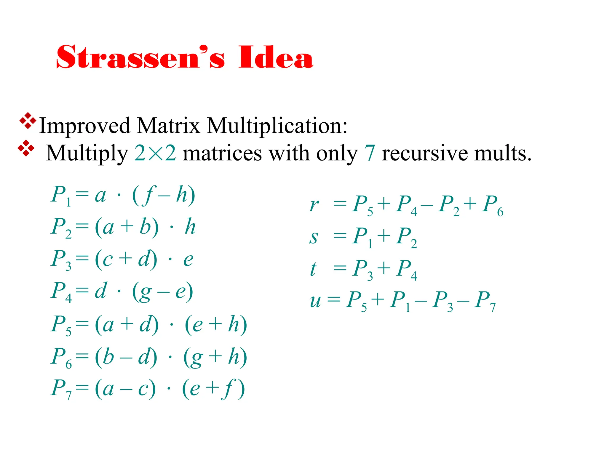
Multiply22 matrices with only 7 recursive mults.
r = P5 + P4 – P2 + P6
s = P1 + P2
t = P3 + P4
u = P5 + P1 – P3 – P7
P1 = a ( f – h)
P2 = (a + b) h
P3 = (c + d) e
P4 = d (g – e)
P5 = (a + d) (e + h)
P6 = (b – d) (g + h)
P7 = (a – c) (e + f )
Improved Matrix Multiplication:
40.
Strassen’s Idea
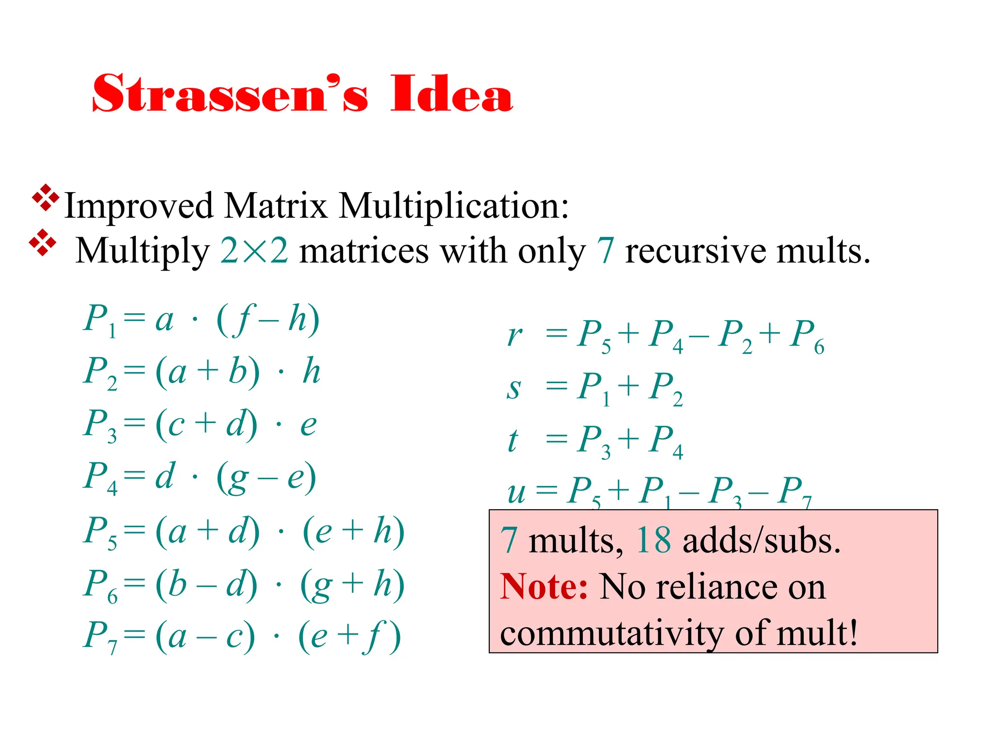
Multiply22 matrices with only 7 recursive mults.
r = P5 + P4 – P2 + P6
s = P1 + P2
t = P3 + P4
u = P5 + P1 – P3 – P7
P1 = a ( f – h)
P2 = (a + b) h
P3 = (c + d) e
P4 = d (g – e)
P5 = (a + d) (e + h)
P6 = (b – d) (g + h)
P7 = (a – c) (e + f )
7 mults, 18 adds/subs.
Note: No reliance on
commutativity of mult!
Improved Matrix Multiplication:
41.
Strassen’s Idea
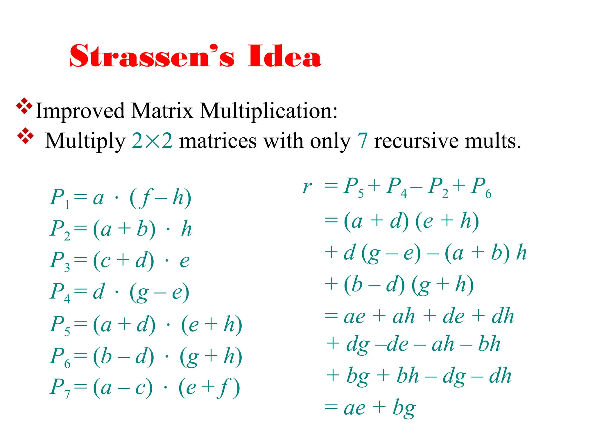
Multiply22 matrices with only 7 recursive mults.
r = P5 + P4 – P2 + P6
= (a + d) (e + h)
+ d (g – e) – (a + b) h
+ (b – d) (g + h)
= ae + ah + de + dh
+ dg –de – ah – bh
+ bg + bh – dg – dh
= ae + bg
P1 = a ( f – h)
P2 = (a + b) h
P3 = (c + d) e
P4 = d (g – e)
P5 = (a + d) (e + h)
P6 = (b – d) (g + h)
P7 = (a – c) (e + f )
Improved Matrix Multiplication:
42.
Strassen’s Algorithm
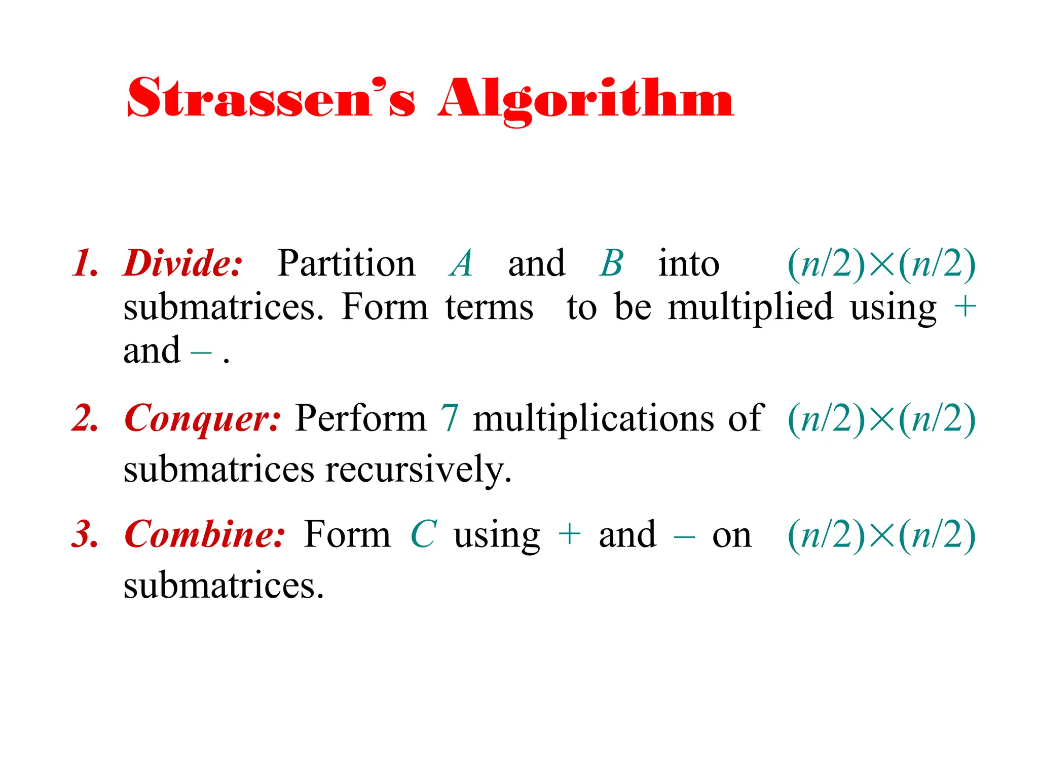
1. Divide:Partition A and B into (n/2)(n/2)
submatrices. Form terms to be multiplied using +
and – .
2. Conquer: Perform 7 multiplications of (n/2)(n/2)
submatrices recursively.
3. Combine: Form C using + and – on (n/2)(n/2)
submatrices.
43.
Strassen’s Algorithm
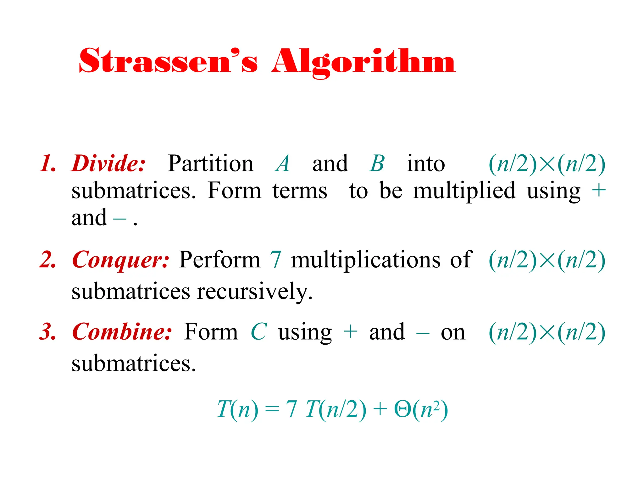
1. Divide:Partition A and B into (n/2)(n/2)
submatrices. Form terms to be multiplied using +
and – .
2. Conquer: Perform 7 multiplications of (n/2)(n/2)
submatrices recursively.
3. Combine: Form C using + and – on (n/2)(n/2)
submatrices.
T(n) = 7 T(n/2) + (n2)
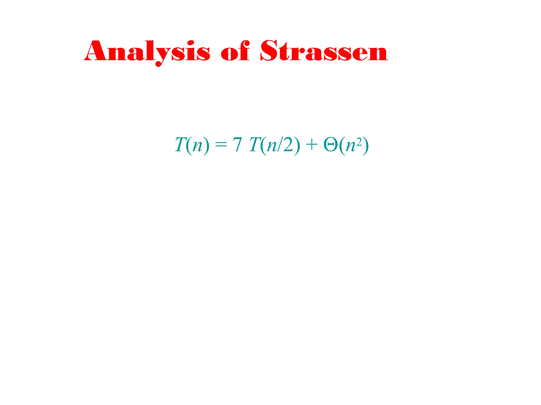
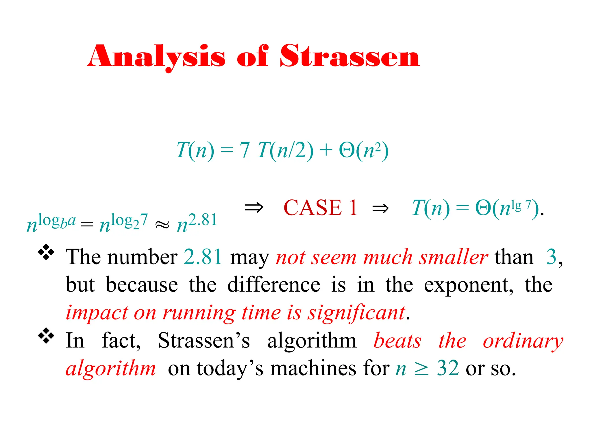
Analysis of Strassen
T(n)= 7 T(n/2) + (n2)
nlogba = nlog27 n2.81
CASE 1 T(n) = (nlg 7).
The number 2.81 may not seem much smaller than 3,
but because the difference is in the exponent, the
impact on running time is significant.
In fact, Strassen’s algorithm beats the ordinary
algorithm on today’s machines for n 32 or so.
47.
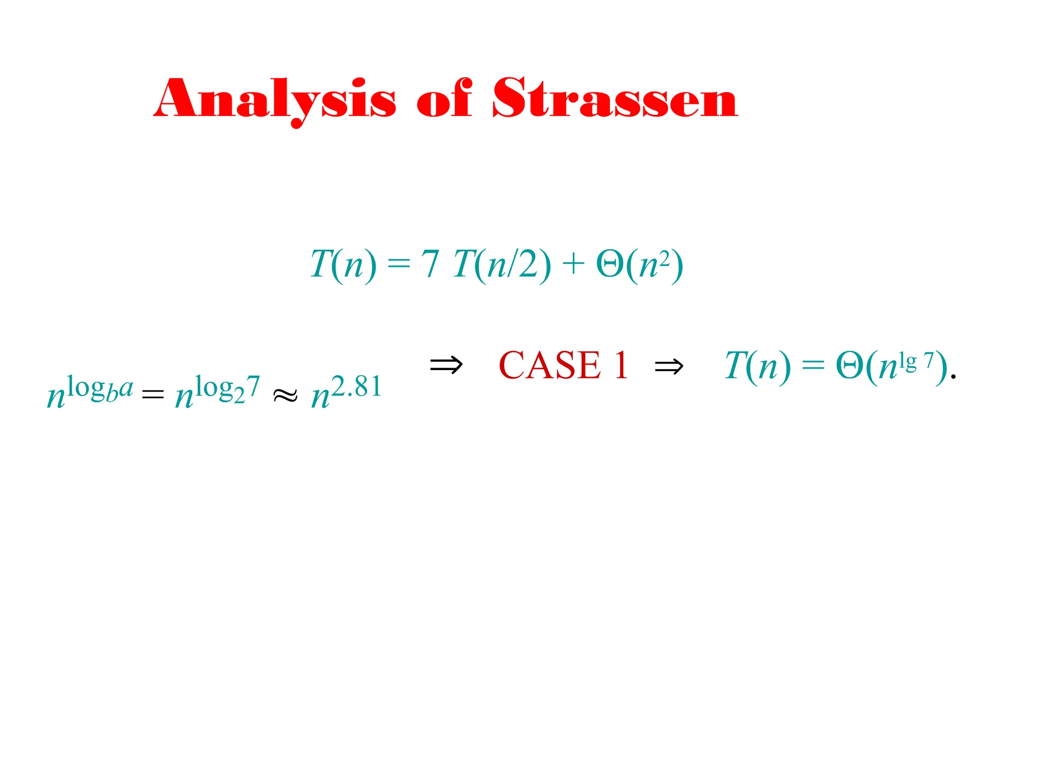
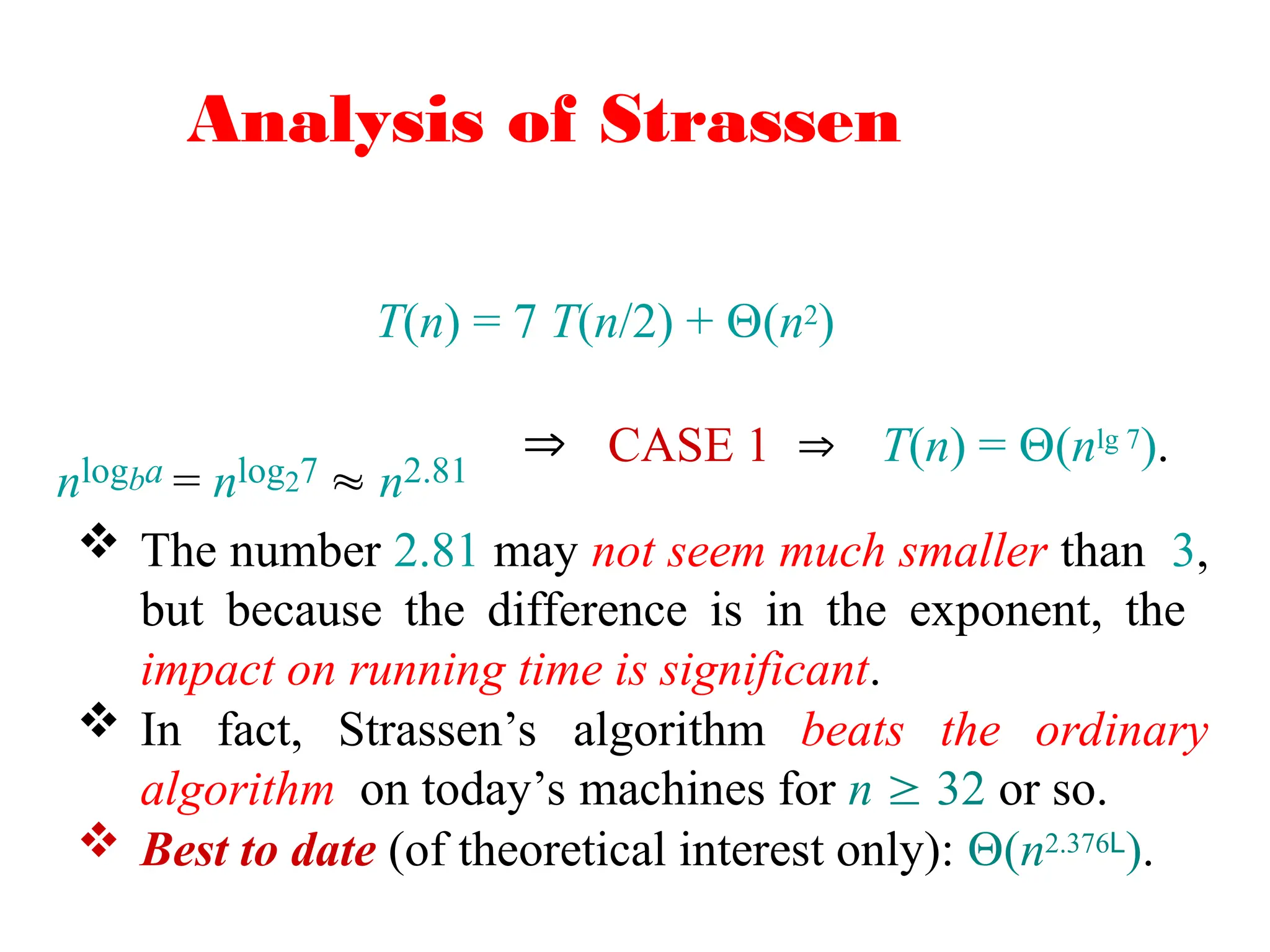
Analysis of Strassen
T(n)= 7 T(n/2) + (n2)
nlogba = nlog27 n2.81
CASE 1 T(n) = (nlg 7).
The number 2.81 may not seem much smaller than 3,
but because the difference is in the exponent, the
impact on running time is significant.
In fact, Strassen’s algorithm beats the ordinary
algorithm on today’s machines for n 32 or so.
Best to date (of theoretical interest only): (n2.376L).
48.
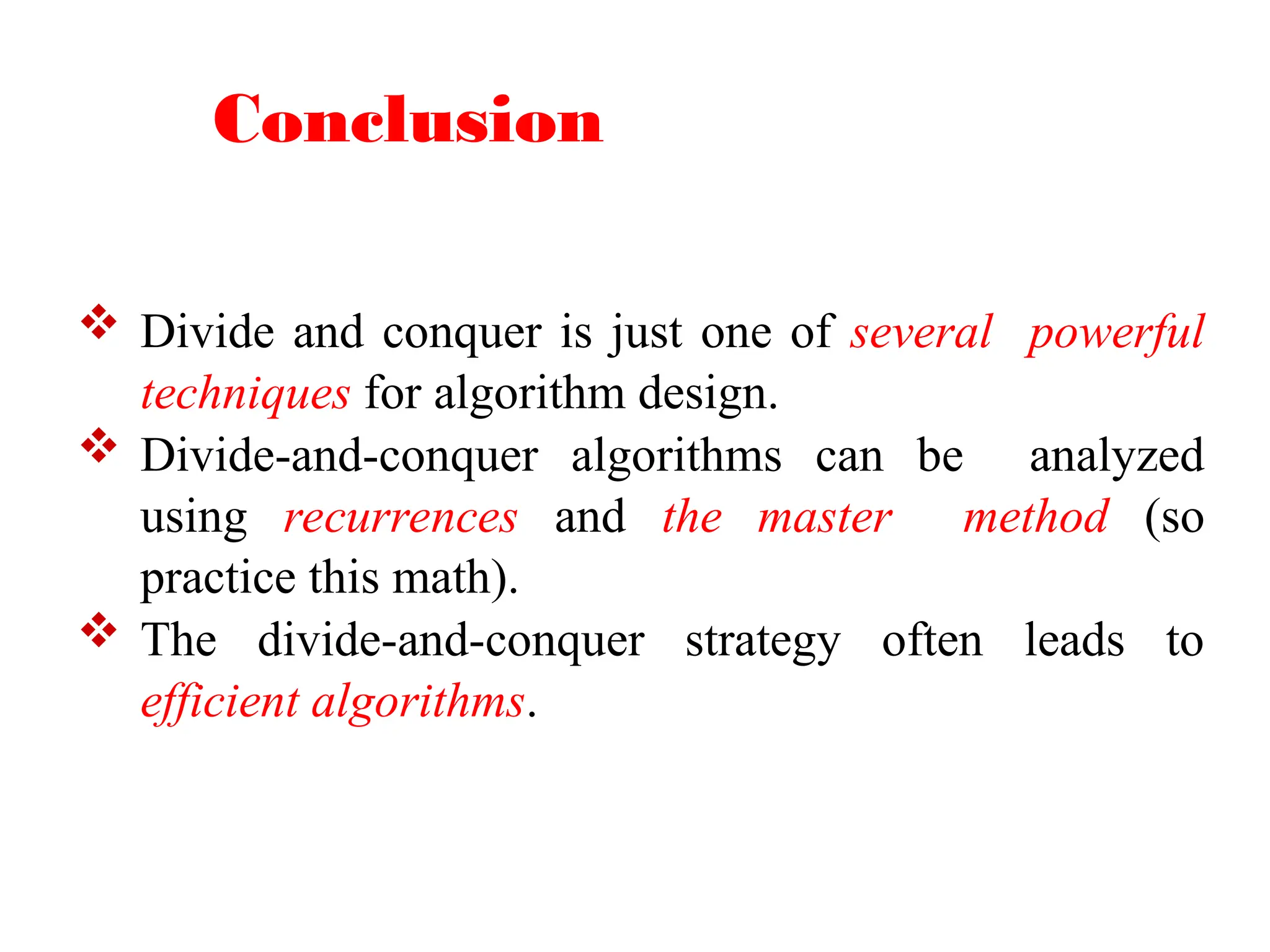
Conclusion
Divide andconquer is just one of several powerful
techniques for algorithm design.
Divide-and-conquer algorithms can be analyzed
using recurrences and the master method (so
practice this math).
The divide-and-conquer strategy often leads to
efficient algorithms.
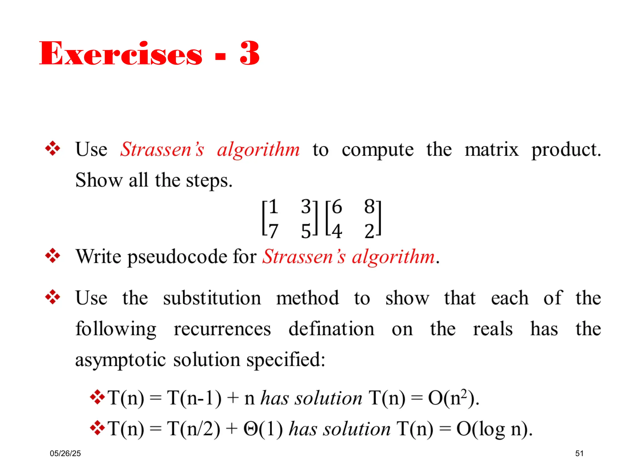
Exercises - 3
05/26/2552
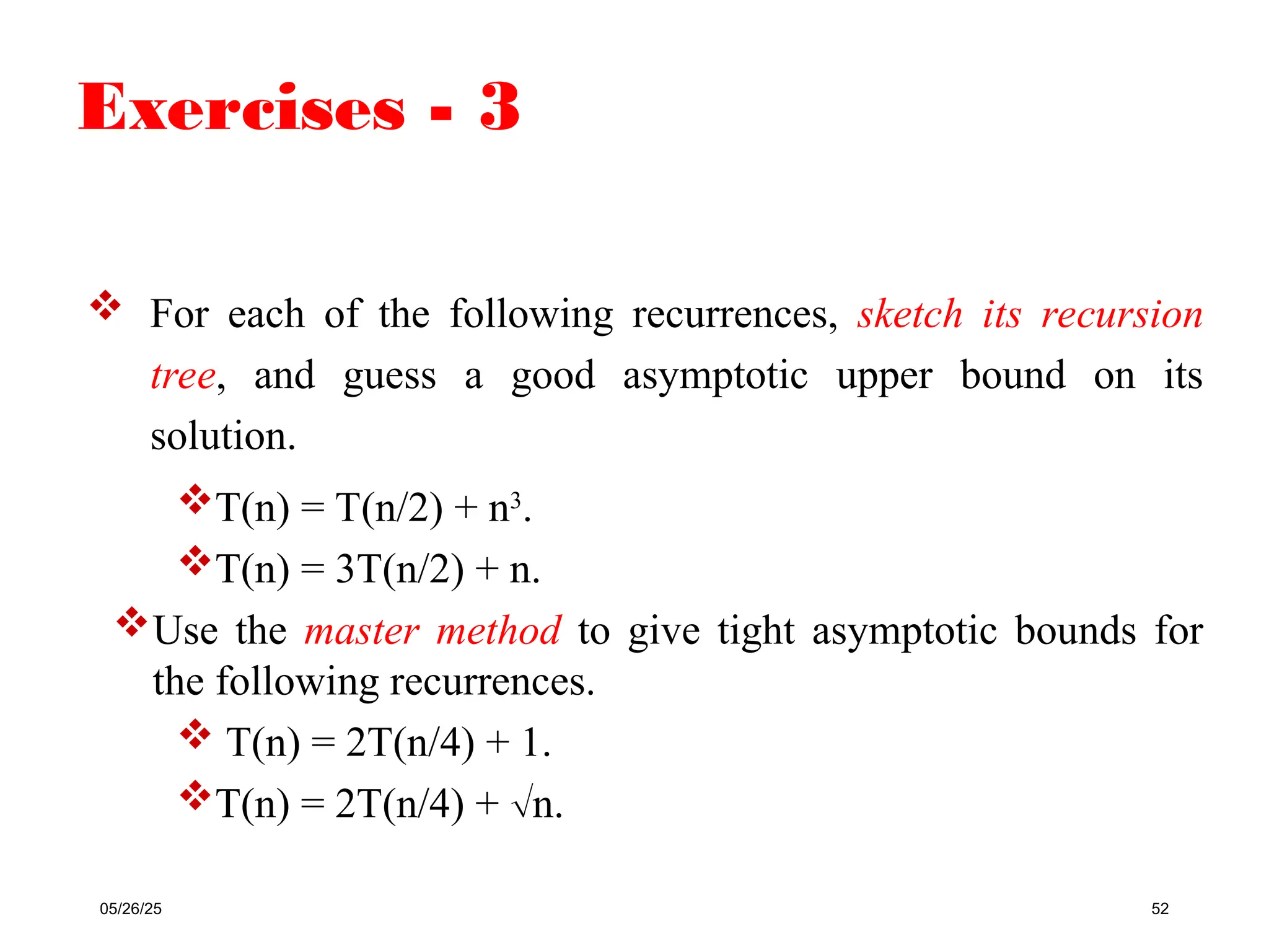
For each of the following recurrences, sketch its recursion
tree, and guess a good asymptotic upper bound on its
solution.
T(n) = T(n/2) + n3
.
T(n) = 3T(n/2) + n.
Use the master method to give tight asymptotic bounds for
the following recurrences.
T(n) = 2T(n/4) + 1.
T(n) = 2T(n/4) + n.
![Merge Sort
Divide the subarray A[p:r] to be sorted into two adjacent
subarrays, each of half the size.
To do so, compute the midpoint q of A[p:r] (taking the average of
p and r), and divide A[p: r] into subarrays A[p:q] and A[q+1: r].
Conquer by sorting each of the two subarrays A[p:q] and
A[q+1:r] recursively using merge sort.
Combine by merging the two sorted subarrays A[p:q] and
A[q+1:r] back into A[p:r], producing the sorted answer.](https://image.slidesharecdn.com/3-chapterthree-divideandconquer-250526181009-6d9d6ea0/75/3-Chapter-Three-Divide-and-Conquer-ppt-4-2048.jpg)
![Master Theorem (reprise)
T(n) = a T(n/b) + f (n)
CASE 1: f (n) = O(nlogba – ), constant > 0
T(n) = (nlogba) .[watershed function grows asymptotically faster than the
driving function]
CASE 2: f (n) = (nlogba lgkn), constant k 0
T(n) = (nlogba lgk+1n) .[if the two functions grow at nearly the same
asymptotic rate]
CASE 3: f (n) = (nlogba + ), constant > 0, and
regularity condition
T(n) = (f(n)) .[the driving function f(n) grows asymptotically faster](https://image.slidesharecdn.com/3-chapterthree-divideandconquer-250526181009-6d9d6ea0/75/3-Chapter-Three-Divide-and-Conquer-ppt-7-2048.jpg)

![Matrix Multiplication
Input: A = [aij], B = [bij].
Output: C = [cij] = A B.
i, j = 1, 2,… , n.
n
cij aik bkj
k 1](https://image.slidesharecdn.com/3-chapterthree-divideandconquer-250526181009-6d9d6ea0/75/3-Chapter-Three-Divide-and-Conquer-ppt-29-2048.jpg)