4
UC Berkeley: IEOR215
Spatial Databases Background
Spatial databases provide structures for storage and analysis of spatial data
Spatial data is comprised of objects in multi-dimensional space
Storing spatial data in a standard database would require excessive amounts of space
Queries to retrieve and analyze spatial data from a standard database would be long and
cumbersome leaving a lot of room for error
Spatial databases provide much more efficient storage, retrieval, and analysis of spatial data
5.
5
UC Berkeley: IEOR215
Types of Data Stored in Spatial Databases
Two-dimensional data examples
– Geographical
– Cartesian coordinates (2-D)
– Networks
– Direction
Three-dimensional data examples
– Weather
– Cartesian coordinates (3-D)
– Topological
– Satellite images
6.
6
UC Berkeley: IEOR215
Spatial Databases Uses and Users
Three types of uses
– Manage spatial data
– Analyze spatial data
– High level utilization
A few examples of users
– Transportation agency tracking projects
– Insurance risk manager considering location risk profiles
– Doctor comparing Magnetic Resonance Images (MRIs)
– Emergency response determining quickest route to victim
– Mobile phone companies tracking phone usage
7.
7
UC Berkeley: IEOR215
Spatial Databases Uses and Users
Three types of uses
– Manage spatial data
– Analyze spatial data
– High level utilization
A few examples of users
– Transportation agency tracking projects
– Insurance risk manager considering location risk profiles
– Doctor comparing Magnetic Resonance Images (MRIs)
– Emergency response determining quickest route to victim
– Mobile phone user determining current relative location of businesses
8.
8
UC Berkeley: IEOR215
Spatial Database Management System
Spatial Database Management System (SDBMS) provides the capabilities of a traditional
database management system (DBMS) while allowing special storage and handling of spatial
data.
SDBMS:
– Works with an underlying DBMS
– Allows spatial data models and types
– Supports querying language specific to spatial data types
– Provides handling of spatial data and operations
9.
9
UC Berkeley: IEOR215
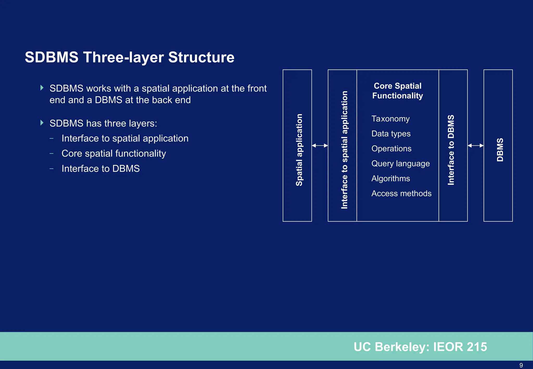
SDBMS Three-layer Structure
SDBMS works with a spatial application at the front
end and a DBMS at the back end
SDBMS has three layers:
– Interface to spatial application
– Core spatial functionality
– Interface to DBMS
Spatial
application
DBMS
Interface
to
DBMS
Interface
to
spatial
application
Core Spatial
Functionality
Taxonomy
Data types
Operations
Query language
Algorithms
Access methods
10.
10
UC Berkeley: IEOR215
Spatial Query Language
Number of specialized adaptations of SQL
– Spatial query language
– Temporal query language (TSQL2)
– Object query language (OQL)
– Object oriented structured query language (O2SQL)
Spatial query language provides tools and structures specifically for working with spatial data
SQL3 provides 2D geospatial types and functions
11.
11
UC Berkeley: IEOR215
Spatial Query Language Operations
Three types of queries:
– Basic operations on all data types (e.g. IsEmpty, Envelope, Boundary)
– Topological/set operators (e.g. Disjoint, Touch, Contains)
– Spatial analysis (e.g. Distance, Intersection, SymmDiff)
12.
12
UC Berkeley: IEOR215
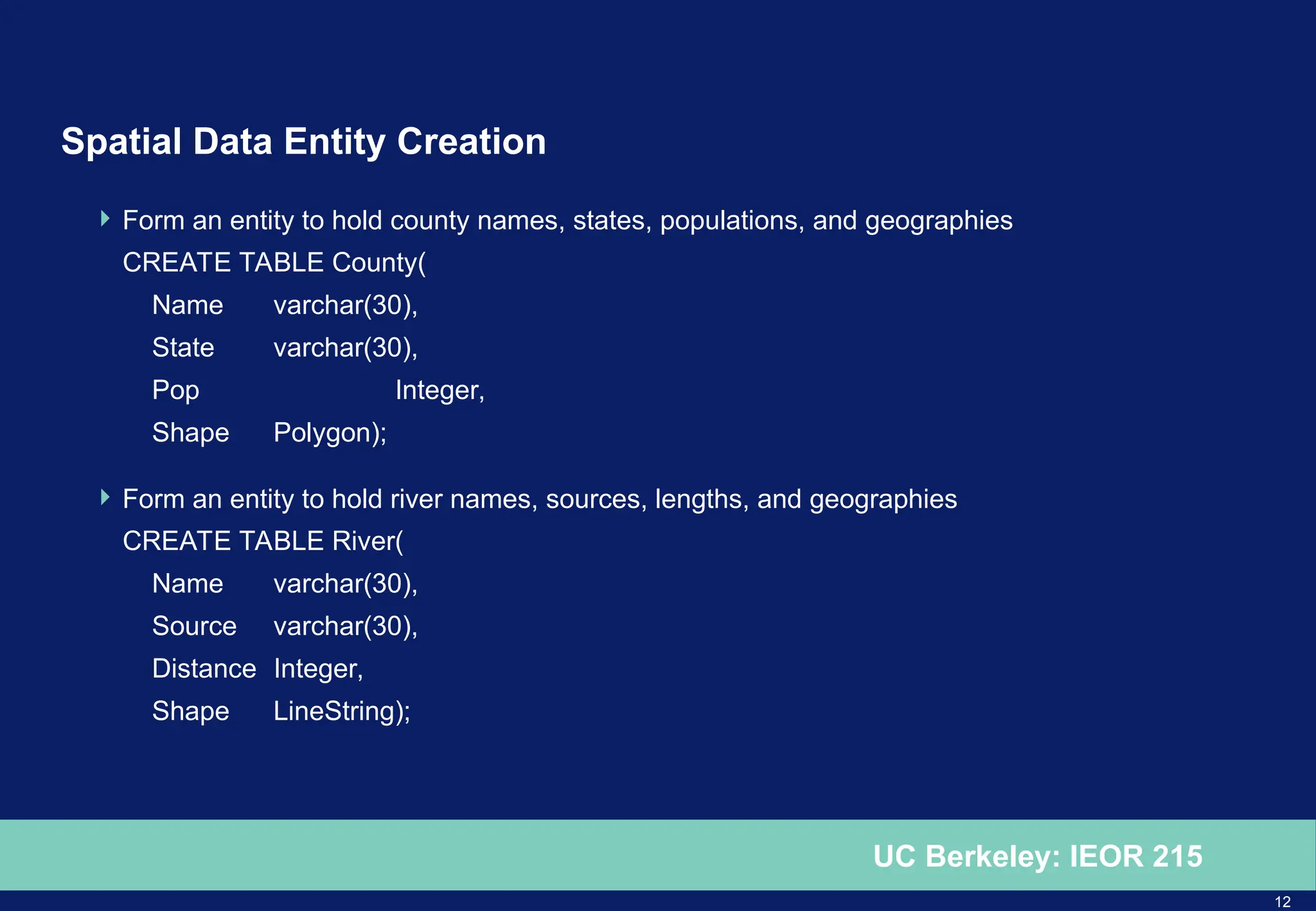
Spatial Data Entity Creation
Form an entity to hold county names, states, populations, and geographies
CREATE TABLE County(
Name varchar(30),
State varchar(30),
Pop Integer,
Shape Polygon);
Form an entity to hold river names, sources, lengths, and geographies
CREATE TABLE River(
Name varchar(30),
Source varchar(30),
Distance Integer,
Shape LineString);
13.
13
UC Berkeley: IEOR215
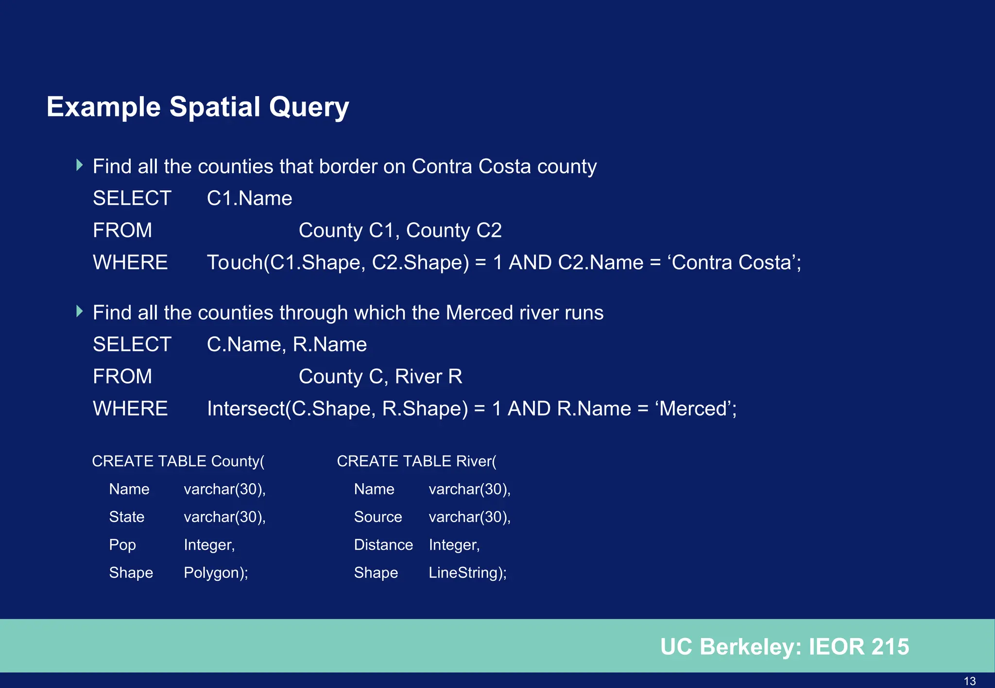
Example Spatial Query
Find all the counties that border on Contra Costa county
SELECT C1.Name
FROM County C1, County C2
WHERE Touch(C1.Shape, C2.Shape) = 1 AND C2.Name = ‘Contra Costa’;
Find all the counties through which the Merced river runs
SELECT C.Name, R.Name
FROM County C, River R
WHERE Intersect(C.Shape, R.Shape) = 1 AND R.Name = ‘Merced’;
CREATE TABLE County(
Name varchar(30),
State varchar(30),
Pop Integer,
Shape Polygon);
CREATE TABLE River(
Name varchar(30),
Source varchar(30),
Distance Integer,
Shape LineString);
14.
14
UC Berkeley: IEOR215
Geographic Information System (GIS) Basics
Common applications
15.
15
UC Berkeley: IEOR215
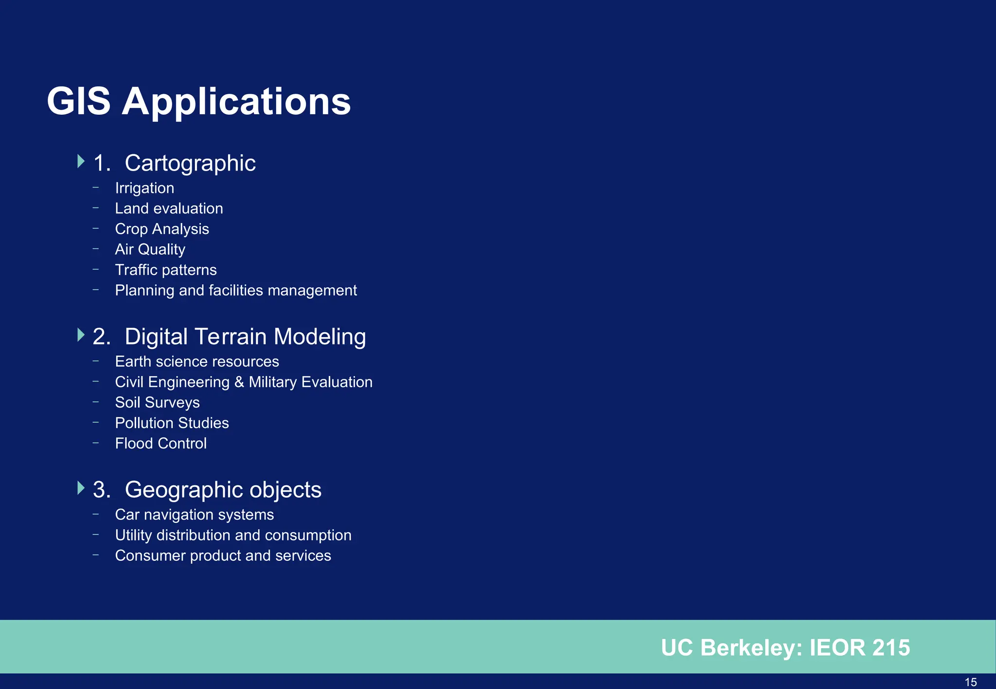
GIS Applications
1. Cartographic
– Irrigation
– Land evaluation
– Crop Analysis
– Air Quality
– Traffic patterns
– Planning and facilities management
2. Digital Terrain Modeling
– Earth science resources
– Civil Engineering & Military Evaluation
– Soil Surveys
– Pollution Studies
– Flood Control
3. Geographic objects
– Car navigation systems
– Utility distribution and consumption
– Consumer product and services
16.
16
UC Berkeley: IEOR215
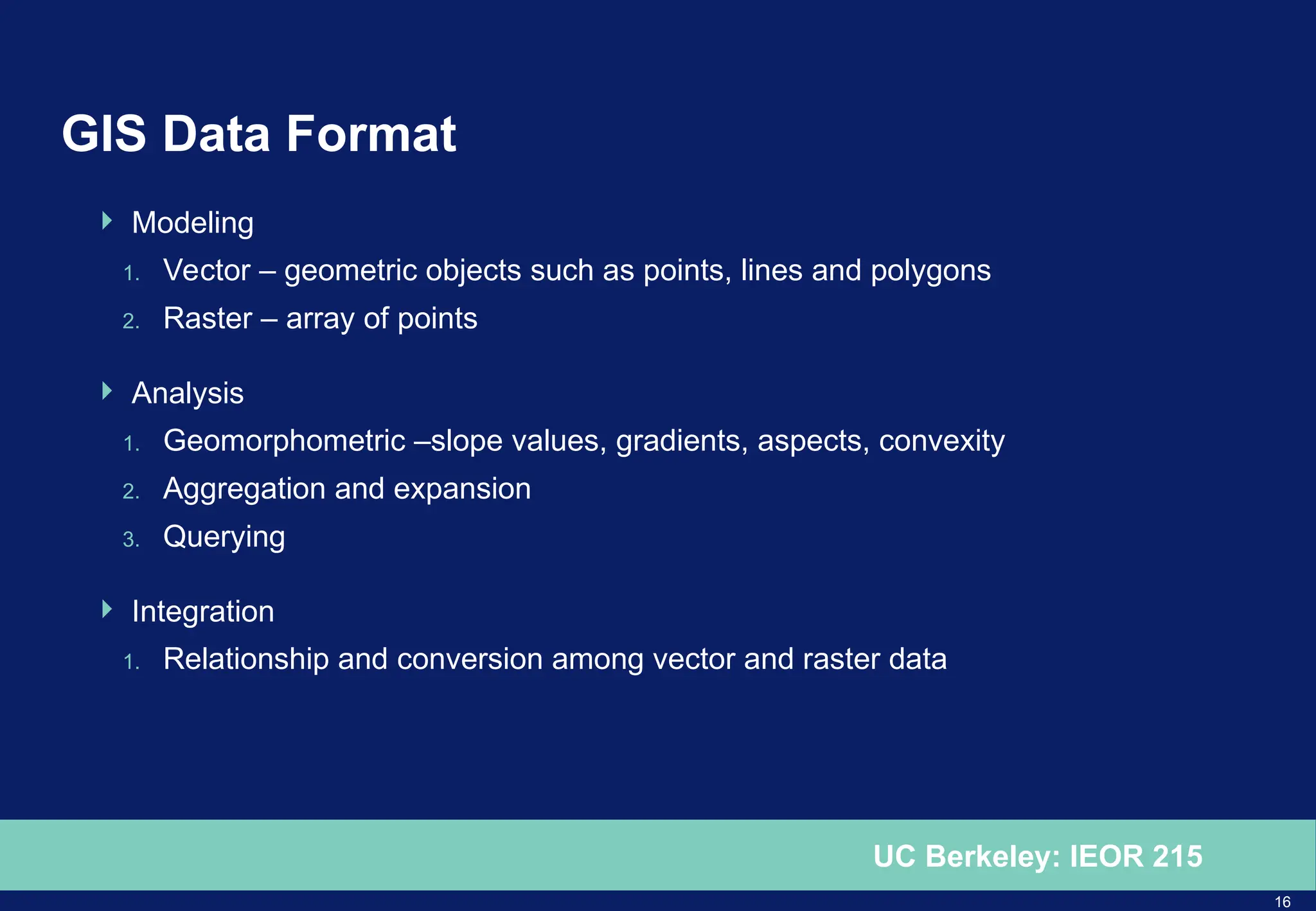
GIS Data Format
Modeling
1. Vector – geometric objects such as points, lines and polygons
2. Raster – array of points
Analysis
1. Geomorphometric –slope values, gradients, aspects, convexity
2. Aggregation and expansion
3. Querying
Integration
1. Relationship and conversion among vector and raster data
17.
17
UC Berkeley: IEOR215
GIS – Data Modeling using Objects & Fields
Name Shape
Pine [(0,2), (4,2), (4,4), (0,4)]
Fir [(0,0), (2,0), (2,2), (0,2)]
Oak [(2,0), (4,0), (4,2), (2,2)
Pine
Fir Oak
(0,4)
(0,2)
(0,0) (2,0) (4,0)
Object Viewpoint Field Viewpoint
Pine: 0<x<4; 2<y<4
Fir: 0<x<2; 0<y<2
Oak: 2<x<4; 0<y<2
Source: “Spatial Pictogram Enhanced Data Models pg 79
18.
18
UC Berkeley: IEOR215
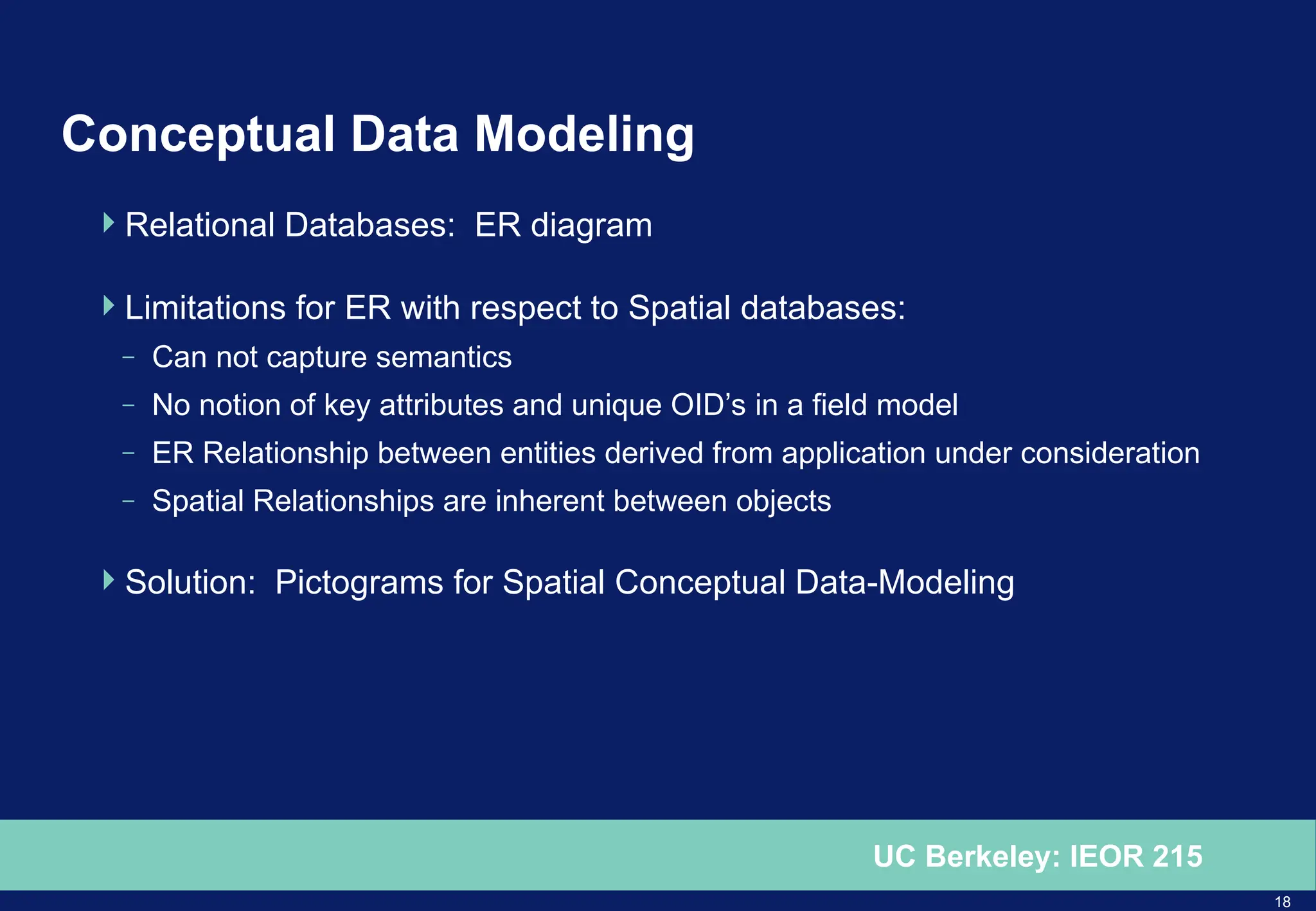
Conceptual Data Modeling
Relational Databases: ER diagram
Limitations for ER with respect to Spatial databases:
– Can not capture semantics
– No notion of key attributes and unique OID’s in a field model
– ER Relationship between entities derived from application under consideration
– Spatial Relationships are inherent between objects
Solution: Pictograms for Spatial Conceptual Data-Modeling
19.
19
UC Berkeley: IEOR215
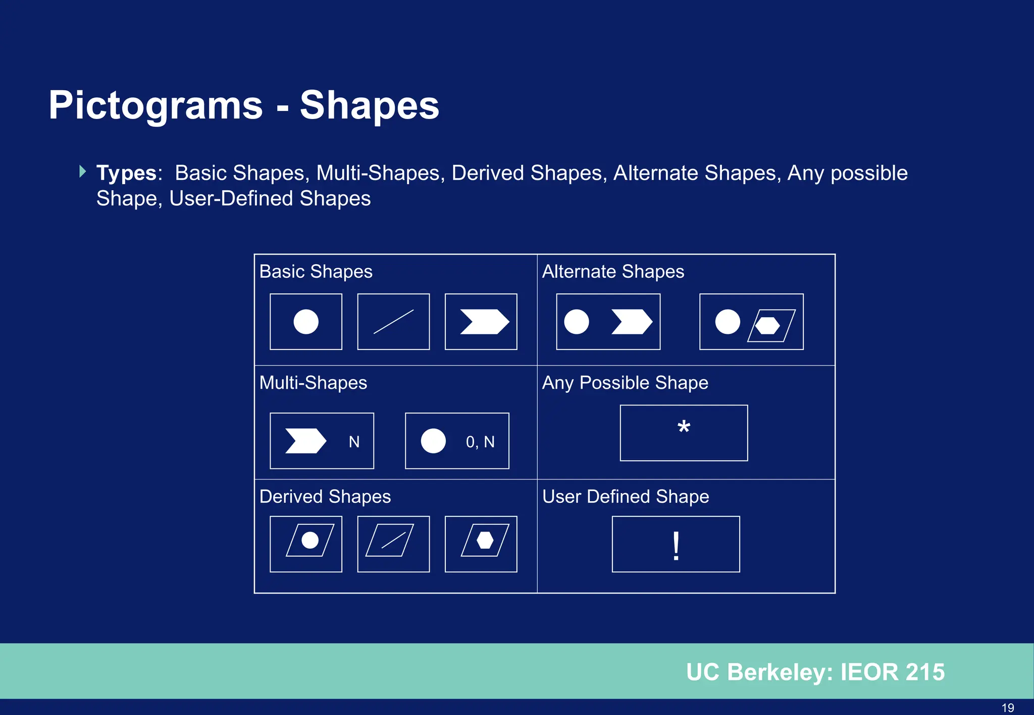
Pictograms - Shapes
Types: Basic Shapes, Multi-Shapes, Derived Shapes, Alternate Shapes, Any possible
Shape, User-Defined Shapes
Basic Shapes Alternate Shapes
Multi-Shapes Any Possible Shape
Derived Shapes User Defined Shape
N 0, N *
!
20.
20
UC Berkeley: IEOR215
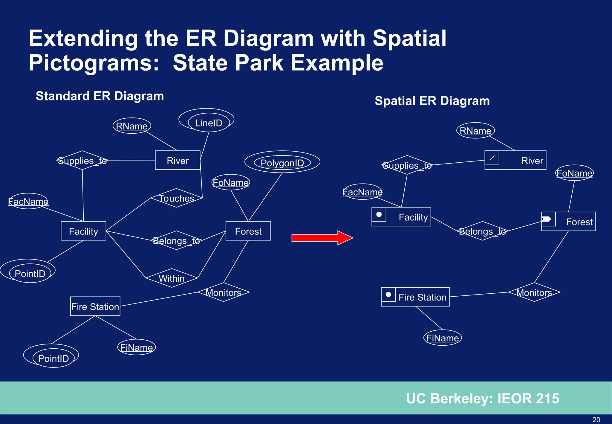
Extending the ER Diagram with Spatial
Pictograms: State Park Example
Forest
Facility
Belongs_to
River
Standard ER Diagram
Supplies_to
Fire Station
Monitors
LineID
PointID
PointID
Within
Touches
FiName
FacName
RName
FoName
Forest
Facility
Belongs_to
River
Supplies_to
Fire Station Monitors
FiName
FacName
RName
FoName
Spatial ER Diagram
PolygonID
21.
21
UC Berkeley: IEOR215
Case Studies
Specific applications of spatial databases
22.
22
UC Berkeley: IEOR215
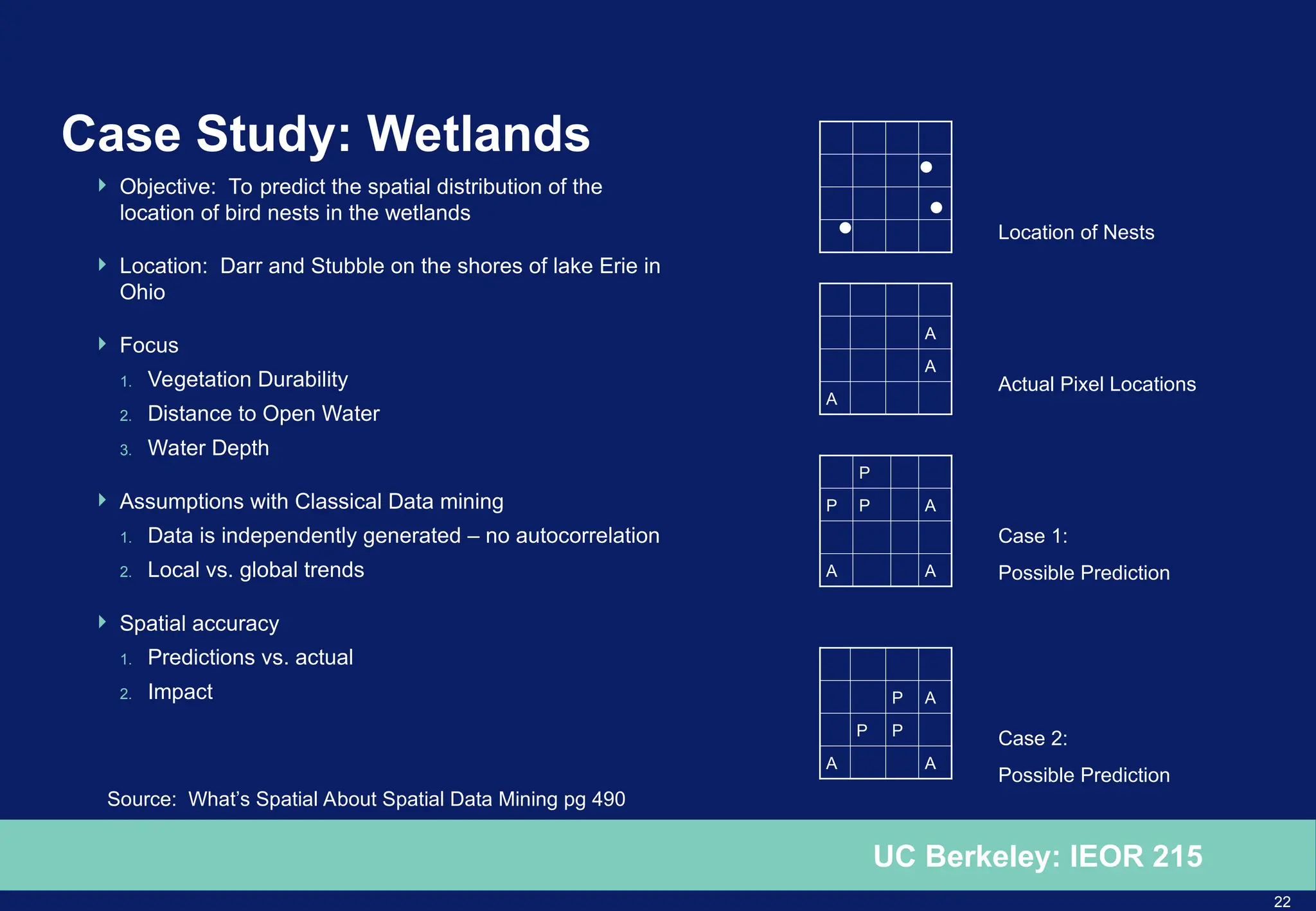
Case Study: Wetlands
Objective: To predict the spatial distribution of the
location of bird nests in the wetlands
Location: Darr and Stubble on the shores of lake Erie in
Ohio
Focus
1. Vegetation Durability
2. Distance to Open Water
3. Water Depth
Assumptions with Classical Data mining
1. Data is independently generated – no autocorrelation
2. Local vs. global trends
Spatial accuracy
1. Predictions vs. actual
2. Impact P A
P P
A A
A
A
A
P
P P A
A A
Location of Nests
Actual Pixel Locations
Case 1:
Possible Prediction
Case 2:
Possible Prediction
Source: What’s Spatial About Spatial Data Mining pg 490
23.
23
UC Berkeley: IEOR215
Case Study: Green House Gas Emission Estimations
Objective:
– To assess the impact of land-use and land cover changes on ground carbon stock and soil
surface flux of CO2, N2O and CH4 in Jambi Province, Indonesia
Methodology:
– Initiated by development of land-use/land cover maps and followed by field measurements
– Spatial database construction development based on 1986 and 1992 land-use/land cover
maps that developed from Landsat MSSR and SPOT
– Weight of sample components of the tree and streams, branches, twigs, etc were estimated
from equations and literature
– Emission rates were developed by plotting and analyzing collected air samples
– Field data measurements and GIS spatial data were combined using a Look Up Table of
Arc/Info.
Source: “Spatial Database Development for green house gas emission Estimation using remote sensing and GIS”
24.
24
UC Berkeley: IEOR215
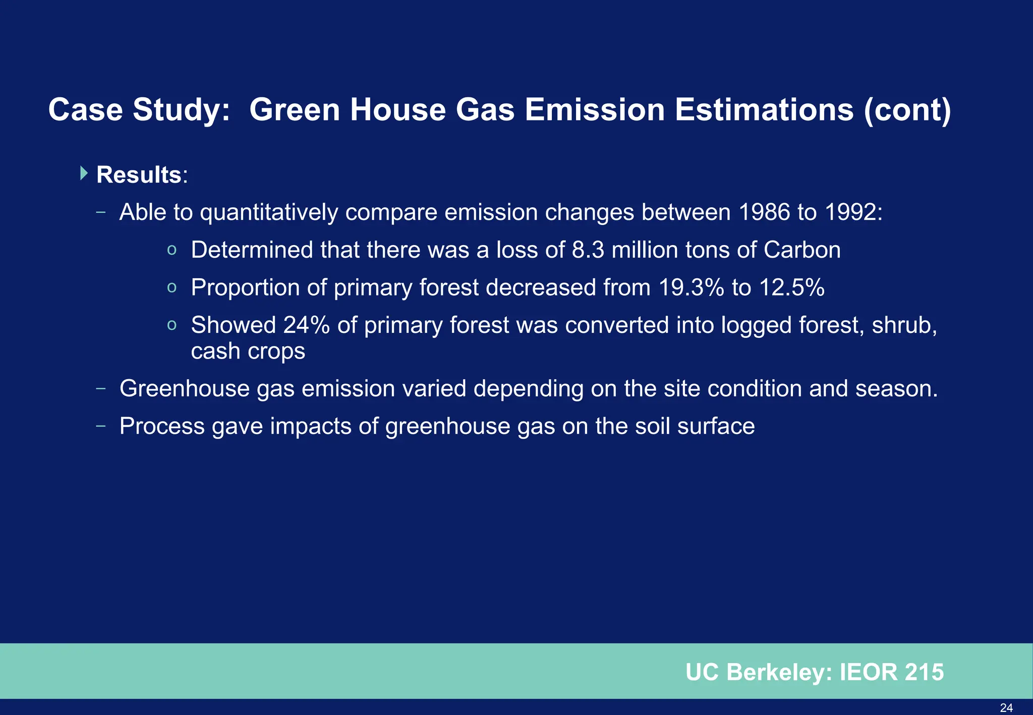
Case Study: Green House Gas Emission Estimations (cont)
Results:
– Able to quantitatively compare emission changes between 1986 to 1992:
o Determined that there was a loss of 8.3 million tons of Carbon
o Proportion of primary forest decreased from 19.3% to 12.5%
o Showed 24% of primary forest was converted into logged forest, shrub,
cash crops
– Greenhouse gas emission varied depending on the site condition and season.
– Process gave impacts of greenhouse gas on the soil surface
25.
25
UC Berkeley: IEOR215
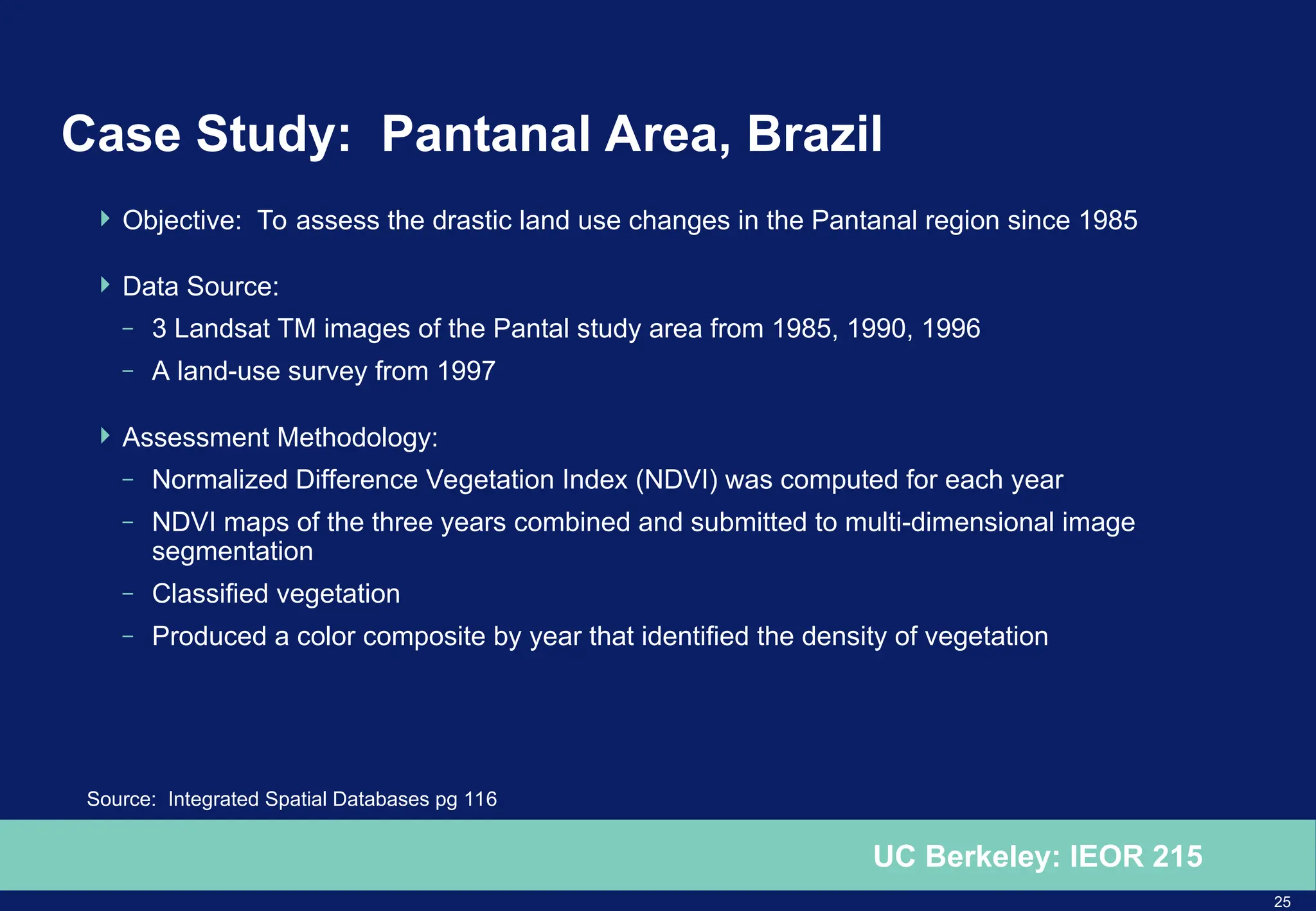
Case Study: Pantanal Area, Brazil
Objective: To assess the drastic land use changes in the Pantanal region since 1985
Data Source:
– 3 Landsat TM images of the Pantal study area from 1985, 1990, 1996
– A land-use survey from 1997
Assessment Methodology:
– Normalized Difference Vegetation Index (NDVI) was computed for each year
– NDVI maps of the three years combined and submitted to multi-dimensional image
segmentation
– Classified vegetation
– Produced a color composite by year that identified the density of vegetation
Source: Integrated Spatial Databases pg 116
26.
26
UC Berkeley: IEOR215
Conclusion
Many varied applications of spatial databases
Stores spatial data in various formats specific to use
Captures spatial data more concisely
Enables more thorough understanding of data
Retrieves and manipulates spatial data more efficiently and effectively
28
UC Berkeley: IEOR215
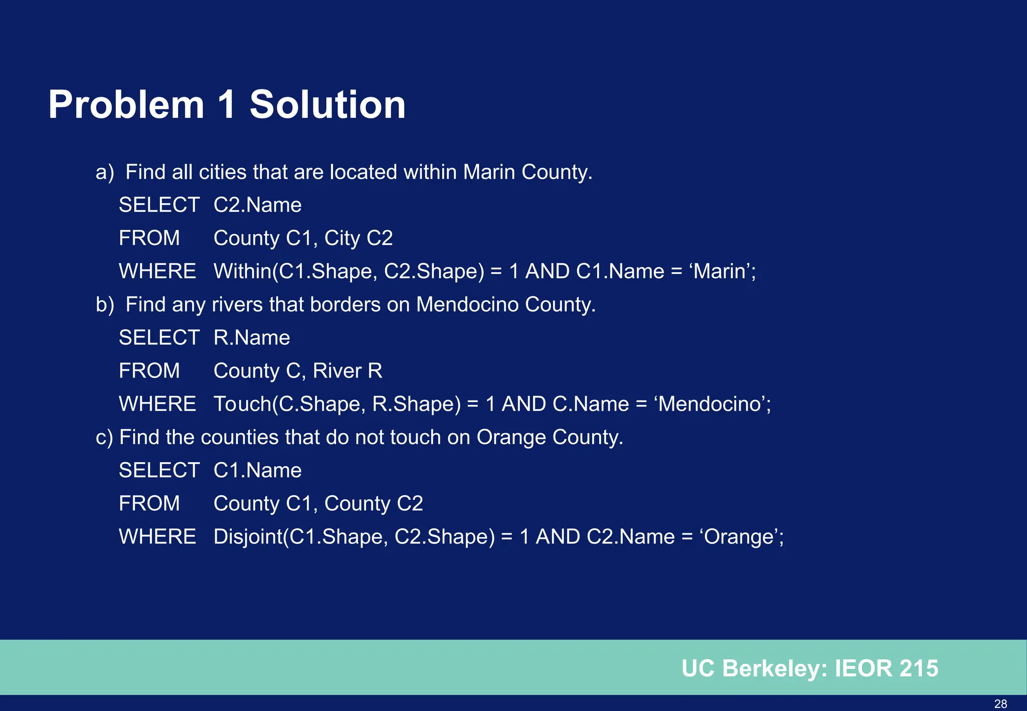
Problem 1 Solution
a) Find all cities that are located within Marin County.
SELECT C2.Name
FROM County C1, City C2
WHERE Within(C1.Shape, C2.Shape) = 1 AND C1.Name = ‘Marin’;
b) Find any rivers that borders on Mendocino County.
SELECT R.Name
FROM County C, River R
WHERE Touch(C.Shape, R.Shape) = 1 AND C.Name = ‘Mendocino’;
c) Find the counties that do not touch on Orange County.
SELECT C1.Name
FROM County C1, County C2
WHERE Disjoint(C1.Shape, C2.Shape) = 1 AND C2.Name = ‘Orange’;
29.
29
UC Berkeley: IEOR215
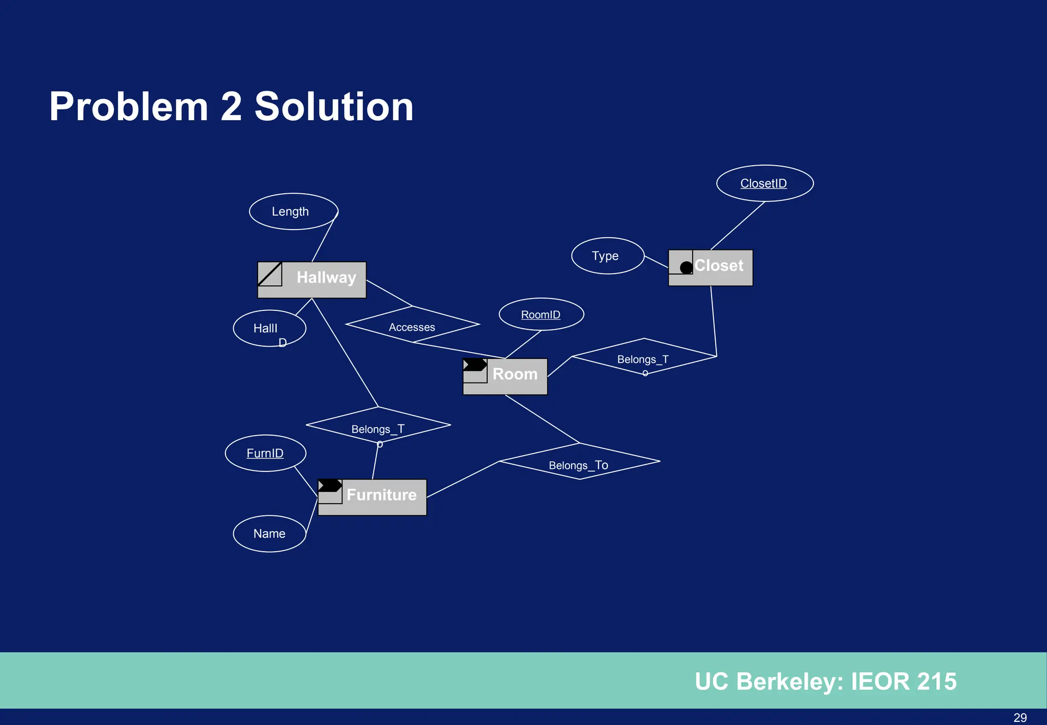
Problem 2 Solution
Room
Hallway
Closet
Furniture
Length
Name
RoomID
FurnID
HallI
D
Type
ClosetID
Belongs_T
o
Belongs_To
Belongs_T
o
Accesses
Editor's Notes
#15 GIS systems are used to collect, model, store and analyze information describing physical properties describing the geographic world. It’s possible to divide GIS into these three main categorize.
In geographic object applications, objects of interest are identified from a physical domain. For example power plants, electroral districts, product distribution districts and city landmarks.
In cartographic and terrain modeling applications, variations in spatial attributes ar captured. For example, soil charactertis, crop density and air quality. Both cartographic and terrain based applications require a field-based representation whereas geographic applications require object based.
#16 GIS data can be represented in two formats: vector and raster.
Vector data represents geometric objects such as points, lines and polygons.
For example if you were modeling a lake, you could use represent it as a polygon or a river by a series of line segments.
Raster data is characterized as an array of points, where each point represents the value of an attribute for a real-world location. Raster images are n-dimensional arrays where each entry is a unit of the image and represents attributes. Two dimensional units are called pizels, while three dimensional units are called voxels. Raster data is typically used with maps of land cover classes such as temperature, rainfall, pasture, urban areas, and standing water.
GIS data undergoes various types of analysis. For example an application such as soil erosion studies, environmental impact studies or hydrological runoff simulations, data undergoes various types of geomorphic analysis – which is the measurement of slope values, gradients, aspect (a complex description of the gradient), convexity (the change of the gradient)
When used for decision support applications it may undergo aggregation and expansion operations using data warehousing as well as querying.
GIS data must integrate both vector and raster data from a variety of sources. Sometimes edges and regions are inferred from a raster image to form a vector model or conversely, raster images are used to update vector models.
#17 GIS data models are usually grouped into broad categories: object and field.
So imagine a forest consisting of clusters of pine, fir and oak trees. What would be the best way to model the forest and capture the aggregate information? Consider a function that maps the underlying geographic space of the forest onto a set consisting of three values (fir, oak and pine). This function would be a field whose varying spatial distribution captures the diversity of the forest. The function itself would be constant over the areas where the tree types were alike and sharply jump into different values when the tree species change.
For an object on the other hand, this function will be composed of a series of polygon that correspond to the different areas with trees.
#18 As we know from this class, ER diagrams are typically used to initial model databases. However for spatial databases ER diagrams are unable at least intuitively to capture some important semantics inherent in spatial modeling. As a result a field model cannot be naturally mapped using the ER model. For example ther is no notion of key attributes and unique OIDS’s in a field model. Although in traditional ER modeling, the relationship between entitites are derived from the application under consideration, in spatial modeling there are always inherent relationships between spatial objects.
So if ER are the best solution for best conceptual spatial data modeling, what is? The answer is using pictograms.
#19 Pictograms are a seriees of shapes that can be used to capture concepts related to spatial geometry.
Basic Shapes: In a vector model the basic elements are point, line and polygon.
Multi-Shapes: To deal with objects which cannot be represented by the basic shapes, this set of aggregate shapes were defined.
Derived Shapes: If the shape of an object is derived form the shapes of other objects it’s pictogram is italicized.
User Defined Shapes: Apart from the basic shapes of point, line and polygon, user-defined shapes are possible.
Any possible Shape: A combination of shapes is represented by a wild card * symbol inside a box, implying that any geometry is possible.
Alternative Shapes: Alternative shapes can be used for the same object depending on certain conditions, for example objects of size less than x units are represented as points while those greater than x units are represented as polygons. They are represented as the concatenation of possible pictograms. Similarly, multiple shapes are needed to represent objects at different scales: for example at higher scales lakes may be presented as points, and at lower scales as polygons.
#22 There are two wetlands – Darr and Stubble on the shores of Lake Erie. Using data collected from April lto June in 1995 and 1996 we want to predict the spatial distribution of a marsh-breed bird, the red-winged blackbird.
A uniform grid was imposed on the 2 wetlands with different types of measurements recorded at pixel. In total, values of 7 attributes were recorded at each pixel. Understanding how the birds interacted with their environment was key to creating the parameters of this studyinig.
Forr example vegetation durability was chosen over vegetation species because specialized knowledge about the bird-nest habits suggested that the choice of next location is more dependent on plant structure, plant resistance to wind and wave action than on the plant species.
So three attributes selected to use in this study: vegetation durability, distance to opn water and water depth.
In this study determining the spatial accuracy – how far the prediction are from the actual nests was critical because of dramatic change in the m eaning of the information if was A or B in this slide.
#23 Landsat MSSR – remote sensing satelittles
MSSR – Multispectrum Scanner Raster
SPOT – System Pour le’Observation de la Terre

![17
UC Berkeley: IEOR 215
GIS – Data Modeling using Objects & Fields
Name Shape
Pine [(0,2), (4,2), (4,4), (0,4)]
Fir [(0,0), (2,0), (2,2), (0,2)]
Oak [(2,0), (4,0), (4,2), (2,2)
Pine
Fir Oak
(0,4)
(0,2)
(0,0) (2,0) (4,0)
Object Viewpoint Field Viewpoint
Pine: 0<x<4; 2<y<4
Fir: 0<x<2; 0<y<2
Oak: 2<x<4; 0<y<2
Source: “Spatial Pictogram Enhanced Data Models pg 79](https://image.slidesharecdn.com/215-spatialdb-250520224249-15c23ae3/75/215-SpatialDB-ppt-case-about-space-for-study-17-2048.jpg)


![Spatial_Data_Analysis_with_open_source_softwares[1]](https://cdn.slidesharecdn.com/ss_thumbnails/8db4d971-8e8c-4fd8-8682-b20e5d6cd65f-161221072847-thumbnail.jpg?width=640&height=640&fit=bounds)