The document provides a comprehensive overview of using the SciPy library in Python for various numerical methods and optimization techniques, including statistics, numerical integration, linear algebra, and solving ordinary differential equations. It includes code snippets demonstrating statistical analysis, matrix operations, least squares fitting, linear regression, and differential equation solutions. The material is aimed at helping users apply these methods for scientific computing and data analysis.

1. Python Crash Course
Scipy
Numerical Methods and Optimization
Using Python
Course Code- 22CSH-259/22ITH-259
By: MSC Dr. Hardeep Kaur (15828)

2. SciPy

3. SciPy: Statistics
>>> from scipy import stats
>>> dir(stats)

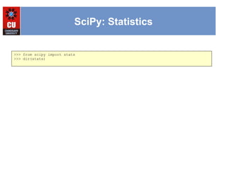
4. SciPy: Statistics
scipy.stats
The
>>> s = sp.randn(100) # same as numpy.random.randn
>>> print len(s)
100
>>> print("Mean : {0:8.6f}".format(s.mean()))
Mean : -0.105170
>>> print("Minimum : {0:8.6f}".format(s.min()))
Minimum : -3.091940
>>> print("Maximum : {0:8.6f}".format(s.max()))
Maximum : 2.193828
>>> print("Variance : {0:8.6f}".format(s.var()))
Variance : 0.863475
>>> print("Std. deviation : {0:8.6f}".format(s.std()))
Std. deviation : 0.929233
>>> from scipy import stats
>>> n, min_max, mean, var, skew, kurt = stats.describe(s)
>>> print("Number of elements: {0:d}".format(n))
Number of elements: 100
>>> print("Minimum: {0:8.6f} Maximum: {1:8.6f}".format(min_max[0], min_max[1]))
Minimum: -3.091940 Maximum: 2.193828
>>> print("Mean: {0:8.6f}".format(mean))
Mean: -0.105170
>>> print("Variance: {0:8.6f}".format(var))
Variance: 0.872197
>>> print("Skew : {0:8.6f}".format(skew))
Skew : -0.146500
>>> print("Kurtosis: {0:8.6f}".format(kurt))
Kurtosis: 0.117884

5. Example: Numerical integration

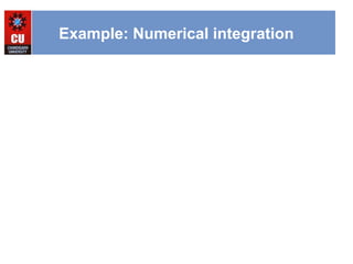
6. Example: Numerical integration
>>> import numpy as np
>>> import scipy as sp
>>> from scipy import integrate # scipy sub-packages have to be imported separately
>>> from scipy import special
>>> result = integrate.quad(lambda x: special.jv(2.5,x), 0, 4.5)
>>> print result
(1.1178179380783249, 7.866317182537226e-09)
>>> I = sqrt(2/pi)*(18.0/27*sqrt(2)*cos(4.5)-4.0/27*sqrt(2)*sin(4.5)+ :
... sqrt(2*pi)*special.fresnel(3/sqrt(pi))[0])
>>> print I
1.11781793809
>>> print abs(result[0]-I)
1.03761443881e-11

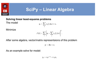
7. SciPy: Linear Algebra
>>> A = matrix('1.0 2.0; 3.0 4.0')
>>> A
[[ 1. 2.]
[ 3. 4.]]
>>> type(A) # file where class is defined
<class 'numpy.matrixlib.defmatrix.matrix'>
>>> B = mat('[1.0 2.0; 3.0 4.0]')
>>> B
[[ 1. 2.]
[ 3. 4.]]
>>> type(B) # file where class is defined
<class 'numpy.matrixlib.defmatrix.matrix'>

8. SciPy – Linear Algebra
>>> A = mat('[1 3 5; 2 5 1; 2 3 8]')
>>> A
matrix([[1, 3, 5],
[2, 5, 1],
[2, 3, 8]])
>>> A.I
matrix([[-1.48, 0.36, 0.88],
[ 0.56, 0.08, -0.36],
[ 0.16, -0.12, 0.04]])
>>> from scipy import linalg
>>> linalg.inv(A)
array([[-1.48, 0.36, 0.88],
[ 0.56, 0.08, -0.36],
[ 0.16, -0.12, 0.04]])
Matrix inversion.

9. SciPy – Linear Algebra
>>> A = mat('[1 3 5; 2 5 1; 2 3 8]')
>>> b = mat('[10;8;3]')
>>> A.I*b
matrix([[-9.28],
[ 5.16],
[ 0.76]])
>>> linalg.solve(A,b)
array([[-9.28],
[ 5.16],
[ 0.76]])
Solving linear system
S = A-1
B where S=[ x y z] and B = [ 10 8 3]

10. SciPy – Linear Algebra
>>> A = mat('[1 3 5; 2 5 1; 2 3 8]')
>>> linalg.det(A)
-25.000000000000004
Finding Determinant

11. SciPy – Linear Algebra
Solving linear least-squares problems
The model
Minimize
After some algebra, vector/matrix representaions of this problem
As an example solve for model:

12. SciPy – Linear Algebra
from numpy import *
from scipy import linalg
import matplotlib.pyplot as plt
c1,c2= 5.0,2.0
i = r_[1:11]
xi = 0.1*i
yi = c1*exp(-xi)+c2*xi
zi = yi + 0.05*max(yi)*random.randn(len(yi))
A = c_[exp(-xi)[:,newaxis],xi[:,newaxis]]
c,resid,rank,sigma = linalg.lstsq(A,zi)
xi2 = r_[0.1:1.0:100j]
yi2 = c[0]*exp(-xi2) + c[1]*xi2
plt.plot(xi,zi,'x',xi2,yi2)
plt.axis([0,1.1,3.0,5.5])
plt.xlabel('$x_i$')
plt.title('Data fitting with linalg.lstsq')
plt.show()

13. SciPy – Singular value decomposition
>>> A = mat('[1 3 2; 1 2 3]')
>>> M,N = A.shape
>>> U,s,Vh = linalg.svd(A)
>>> Sig = mat(linalg.diagsvd(s,M,N))
>>> U, Vh = mat(U), mat(Vh)
>>> print U
[[-0.70710678 -0.70710678]
[-0.70710678 0.70710678]]
>>> print Sig
[[ 5.19615242 0. 0. ]
[ 0. 1. 0. ]]
>>> print Vh
[[ -2.72165527e-01 -6.80413817e-01 -6.80413817e-01]
[ -6.18652536e-16 -7.07106781e-01 7.07106781e-01]
[ -9.62250449e-01 1.92450090e-01 1.92450090e-01]]
Singular Value Decompostion (SVD) can be thought of as an extension of the
eigenvalue problem to matrices that are not square. Let A be an M x N matrix.
SVD of A can be written as
With U = AH
A and V= AAH
and  is the matrix of eigenvectors

14. Example: Linear regression
import scipy as sp
from scipy import stats
import pylab as plt
n=50 # number of points
x=sp.linspace(-5,5,n) # create x axis data
a, b=0.8, -4
y=sp.polyval([a,b],x)
yn=y+sp.randn(n) #add some noise
(ar,br)=sp.polyfit(x,yn,1)
yr=sp.polyval([ar,br],x)
err=sp.sqrt(sum((yr-yn)**2)/n) #compute the mean square error
print('Linear regression using polyfit')
print(‘Input parameters: a=%.2f b=%.2f’ % (a,b))
print(‘Regression: a=%.2f b=%.2f, ms error= %.3f' % (ar,br,err))
plt.title('Linear Regression Example')
plt.plot(x,y,'g--')
plt.plot(x,yn,'k.')
plt.plot(x,yr,'r-')
plt.legend(['original','plus noise', 'regression'])
plt.show()
(a_s,b_s,r,xx,stderr)=stats.linregress(x,yn)
print('Linear regression using stats.linregress')
print('parameters: a=%.2f b=%.2f’ % (a,b))
print(‘regression: a=%.2f b=%.2f, std error= %.3f' % (a_s,b))

15. Example: Least squares fit
from pylab import *
from numpy import *
from matplotlib import *
from scipy.optimize import leastsq
fp = lambda v, x: v[0]/(x**v[1])*sin(v[2]*x) # parametric function
v_real = [1.7, 0.0, 2.0]
fn = lambda x: fp(v_real, x) # fn to generate noisy data
e = lambda v, x, y: (fp(v,x)-y) # error function
n, xmin, xmax = 30, 0.1, 5 # Generate noisy data to fit
x = linspace(xmin,xmax,n)
y = fn(x) + rand(len(x))*0.2*(fn(x).max()-fn(x).min())
v0 = [3., 1, 4.] # Initial parameter values
v, success = leastsq(e, v0, args=(x,y), maxfev=10000) # perform fit
print ‘Fit parameters: ', v
print ‘Original parameters: ', v_real
X = linspace(xmin,xmax,n*5) # plot results
plot(x,y,'ro', X, fp(v,X))
show()

16. SciPy: Ordinary Differential Equations
Simple differential equations can be solved numerically using the Euler-Cromer method, but more
complicated differential equations may require a more sophisticated method. The scipy library for Python
contains numerous functions for scientific computing and data analysis. It includes the function odeint for
numerically solving sets of first-order, ordinary differential equations (ODEs) using a sophisticated algorithm.
rewritten as the following two first-order differential equations,
The function y will be the first element y[0] (remember that the lowest index of an array is zero, not
one) and the derivative y ′ will be the second element y[1]. You can think of the index as how many
derivatives are taken of the function. In this notation, the differential equiations are
from scipy import odeint
from pylab import * # for plotting commands
def deriv(y,t): # return derivatives of the array y
a = -2.0
b = -0.1
return array([ y[1], a*y[0]+b*y[1] ])
time = linspace(0.0,10.0,1000)
yinit = array([0.0005,0.2]) # initial values
y = odeint(deriv,yinit,time)
figure()
plot(time,y[:,0]) # y[:,0] is the first column of y
xlabel(‘t’)
ylabel(‘y’)
show()

17. Introduction to language
End