Downloaded 18 times

![Bifurcationmethodsin nonlinearflightdynamics 547
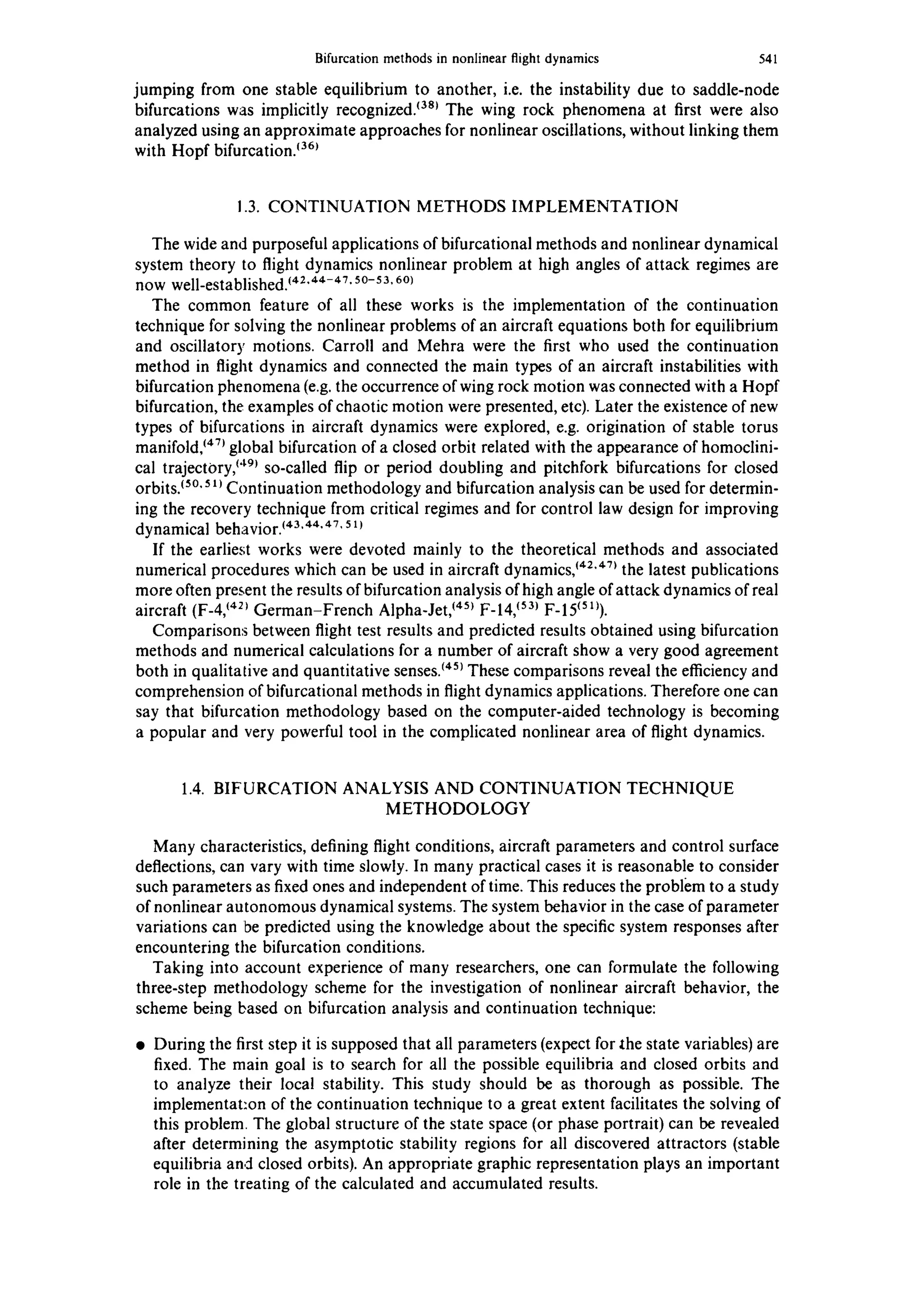
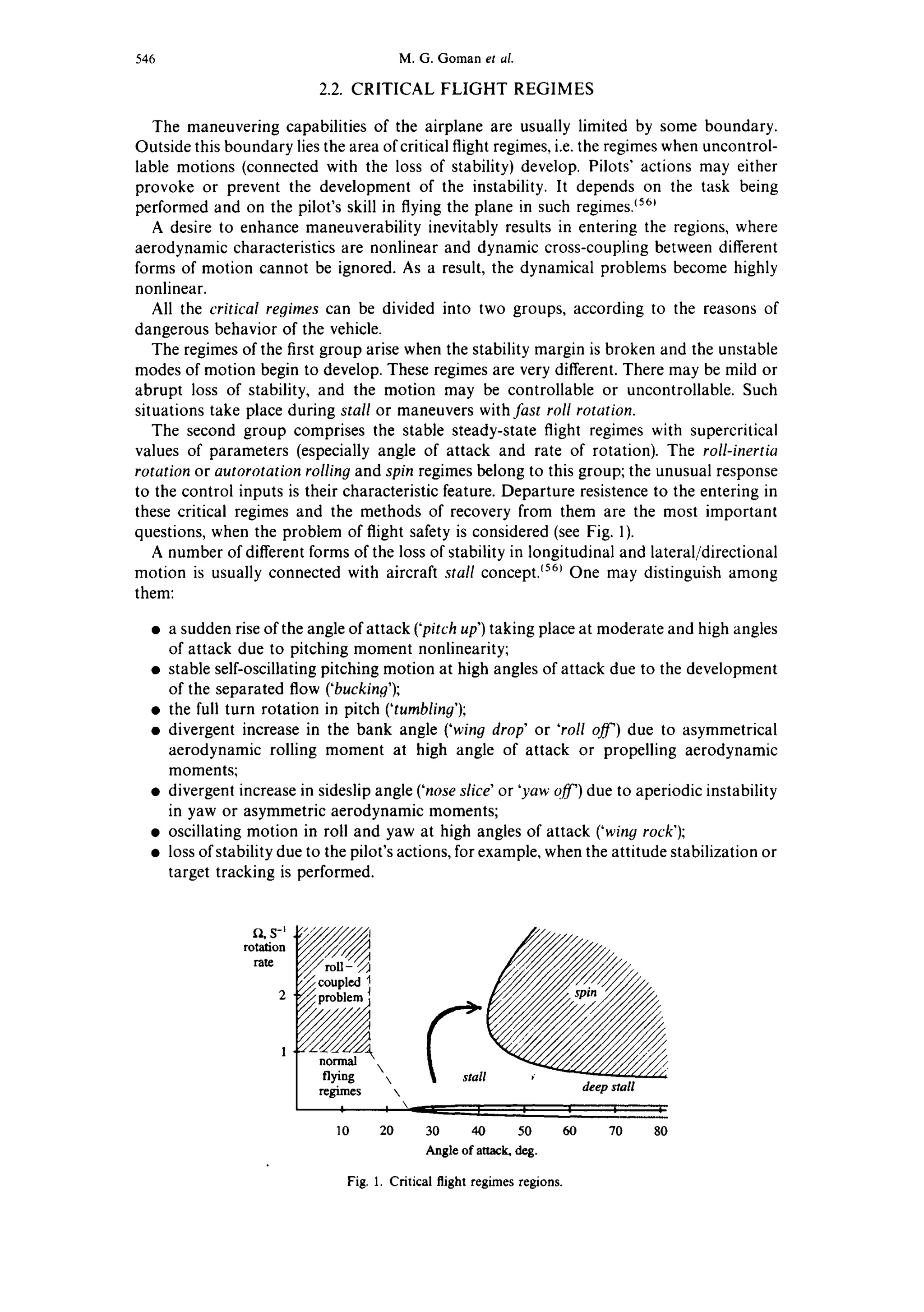
There are also terms used in the flight dynamics for describing the aircraft behavior after
stall, i.e. post-stall gyration, spin and deep stall. The post-stall gyration is a transient
rotational motion of aircraft to the developed spin mode. The developed spin can possess
very different features. It can be steady with constant parameters or 'agitated',flat or steep,
erected or inverted. 'Agitated' spin mode can be with regular and 'irregular' oscillations.
Deep stall is art aircraft equilibrium flight at high critical angle of attack without rotation.
The possibiltty of the loss of stability and controllability at high roll rate (roll-coupled
problem) is also well-known. This phenomenon is especially dangerous for supersonic
aircraft with elongated ellipsoid of inertia and high level of lateral aerodynamic stability,
which bring about cross-coupling of longitudinal and lateral motions.
Roll-inertia rotation or autorotation rolling of the airplane (the trajectory being approxi-
mately horizontal and angles of incidence below stalling) is similar to the developed
spin modes. The rotation can occur despite neutral or anti-rotation aileron and rudder
deflections.
In both cases there are autorotational regimes, the difference is only in the nature of the
aerodynamic moment that supports the rotation.
All types of motion mentioned above can be connected with qualitative features of
motion equations, i.e. the different steady-state aircraft motions and bifurcations, changing
their stability conditions.
2.3. DYNAMICS OF SYMMETRICAL FLIGHT IN A VERTICAL PLANE
To demonstrate the nonlinear dynamics behavior of symmetrical flight using the bifurca-
tional and global stability analysis methods one can consider two simplified examples
arising basically from trajectory or angular pitch motion.
Taking into account that in symmetrical flight the state variables are equal to zero:
q~w = 0, ~ = 0, fl = 0, Pw = rw = 0, and 0w = 7• [- n,n], where ~' is a path angle, the
following equations of motion can be extracted from the complete system (Eqs (1)-(4)):
Tcos • CopS )
m~'=g mg ~ V2-sin)'
";' g (.T sin ~ CLpS )
= -- + V2 _ cos 7
V mg
4=q-,}
= Cm(~,q, fie)p V2S?
2Ir
(10)
)(E = VCOS~
//= Vsin7
The first two equations of this system are responsible for the so-called phugoid trajectory
motion, the second two equations are responsible for short-period rotational motion. At
relatively large velocities of flight these two subsystems approximately can be considered
separately.
2.4. NONLINEAR PHUGOID MOTION
This problem was first considered by Zhukovsky and Lanchester and later became one of
the classical examples of second-order nonlinear systems, illustrating the qualitative
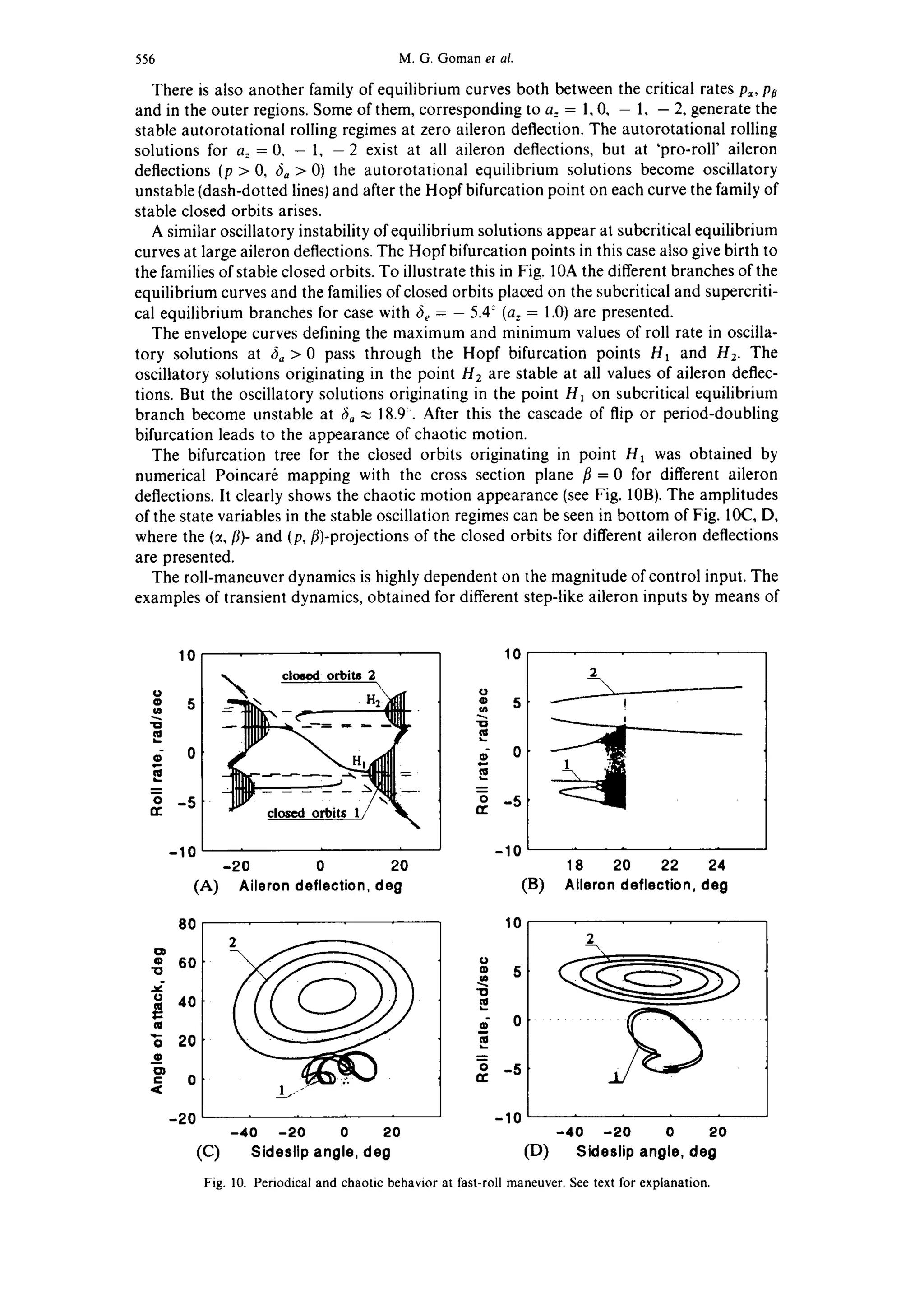
methods of analysis.](https://image.slidesharecdn.com/1997gomanzagainovkhramtsovsky-applicationofbifurcationmethodstononlinearflightdynamicsproblems-131005035700-phpapp01/75/1997-9-2048.jpg)
![548 M.G. Goman et al.
Assuming that the angle of attack is a constant, and therefore the lift and drag coefficients
are also constants, the following nondimensional autonomous second order nonlinear
system can be used for investigation of phugoid motion with large amplitudes:
--cl~) = b - ay 2 - sin 7
dr
d), cos 7
dr - y Y
(11)
T CD.
where b m9 is the thrust-to-weight ratio considered as a parameter (:t <~1), a ~. ts the
2mg
drag-to-lift ratio, r = VOqt is the nondimensional time and Vo = ~]pSCLis the velocity of
horizontal flight.
The equilibrium solutions of this system at different values of parameters a and b are
~:orresponded to straightline trajectories with climb (7 > 0) or glide ('/< 0) path angle. There
is some critical boundary in parameter space exceeding which makes the equilibrium
oscillatory unstable. At some values of parameters a, b another kind of steady solution
appears. These are the stable and unstable closed orbits, enclosing the cylindrical state space
or equilibrium points. The stable closed orbits, enclosing the cylinder correspond to the
curvilinear trajectories with recurring loops, the so-called 'dead loops'. The unstable closed
orbits, enclosing the cylinder or the equilibrium points, separate the regions of attraction of
the stable equilibrium points and the stable closed orbits, enclosing the cylinder.
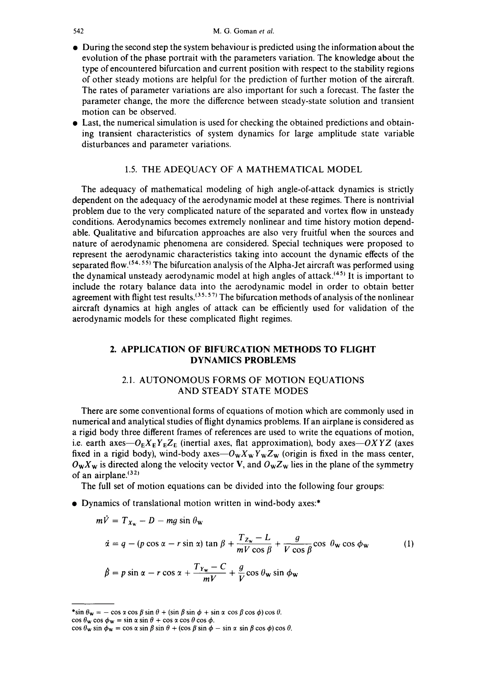
In Fig. 2 the bifurcation diagram is presented when the parameter b is varied for a = 0.2.
The path angle of equilibrium straightlinear flight ~ becomes positive, when b >/a. When
parameter b exceeds the critical value bcr, ,~ 0.4 stable and unstable closed orbits, enclosing
the cylinder, appear. After that the stable cycle moves up and the unstable one moves down
along velocity axes y. There is some bifurcation moment (bcr2~ 0.42), when the unstable
cycle involves the critical points y = 0, 7= + ~/2. These critical points in state space
correspond to the cusp points on the flight trajectory, where the path angle varies from
7 = ~/2 to ?, = - n/2 instantaneously. In real flight it is impossible due to inertiality of
angular pitch motion. In this case, corresponding to the well-known aircraft maneuvers
y n
rd2
-~,e2
stable closed orbits,
surroundingcylinder
/
, i "
closed orbits ~ J
stable e.quilibria~ unstable|I~I I
.------ ............ equilibria
4.2 0 0.2 0.4 0.6 0.8 Wmg
Fig. 2. Equilibrium and periodical solutions as a function of parameter b with a = 0.2.](https://image.slidesharecdn.com/1997gomanzagainovkhramtsovsky-applicationofbifurcationmethodstononlinearflightdynamicsproblems-131005035700-phpapp01/75/1997-10-2048.jpg)

![550 M.G. Gomanet al.
560
420
280
140
a = 0.2o b = 0.0
560
420
280
140
i I I i
240 480 720 960
(A) L,m (B)
a=0.2, b=0.7
I I I I
240 480 720 960
L,m
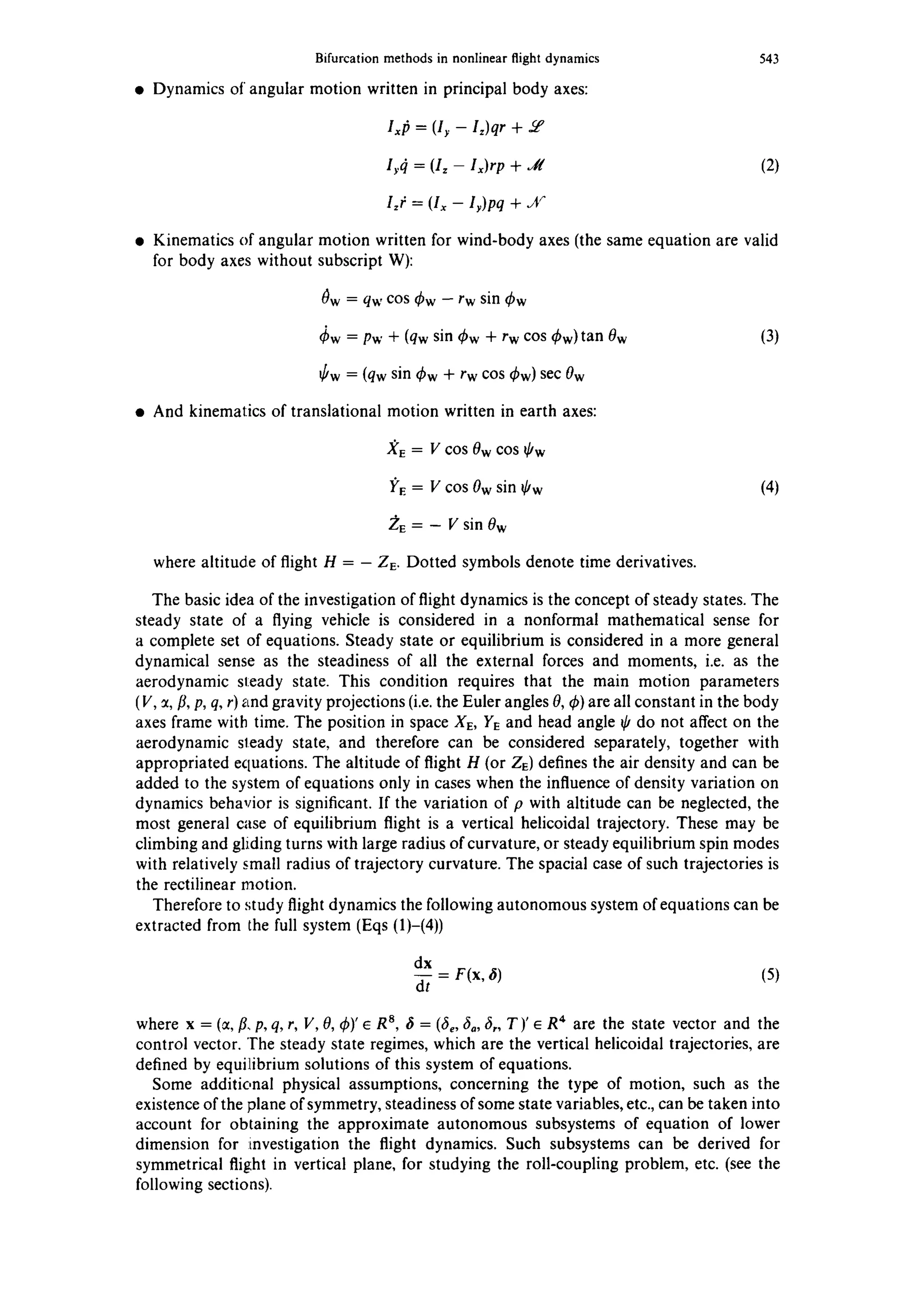
Fig.4. Flighttrajectorieswith'dead' loops,A) b = 0, B) b = 0.7.
The understanding of nonlinear dynamics and the prediction of the region of attraction
generated by the critical deep stall regime are very important for stall prevention and also
for design of the recovery control from deep stall. To form the approximate equations one
can consider that the velocity of flight is not varied and the path is rectilinear:
~=q
( t~1: Cm(~)@ CmqV -[- Cm6e~e T SC
(12)
The qualitative analysis of nonlinear dynamics in this case can easily be done in the phase
plane of the state variables (~ and q) (see Fig. 5). There are three different equilibrium points
:~,, ~2, ~3, two of which (al, ~3) are stable loci and one (~2) is the saddle point. This unstable
saddle-type equilibrium point generates very informative phase trajectories W~, which are
going in it along the eigenvector, corresponding to the stable eigenvalue. Two other
trajectories W uare going out from saddle point along the eigenvector, corresponding to the
unstable eigenvector. These trajectories are attracted by stable points ~1, ~3. All these
singular trajectories can be computed by means of integrating the system (12). Initial
conditions for reconstruction of these singular trajectories are taken in a small vicinity of
the saddle point ~2 with displacements along the stable and unstable eigenvectors. The
trajectories W u are integrated in the positive time direction, and W s are integrated in the
backward time direction. Note, that the region of attraction of the deep stall regime ~3
(dashed area in Fig. 5) depends on the altitude and velocity of flight, and the magnitude of
the pitch damping derivative Cm.
2.6. THE GENERAL CASE OF THE LONGITUDINAL MOTION
As was mentioned above the interaction between the phugoid and angular modes is more
significant for flight with low velocities. In this case the large variation of angle of attack can
arise due to trajectory distortion. For example, such trajectory distortion accompanies the
tail-slide maneuvers.
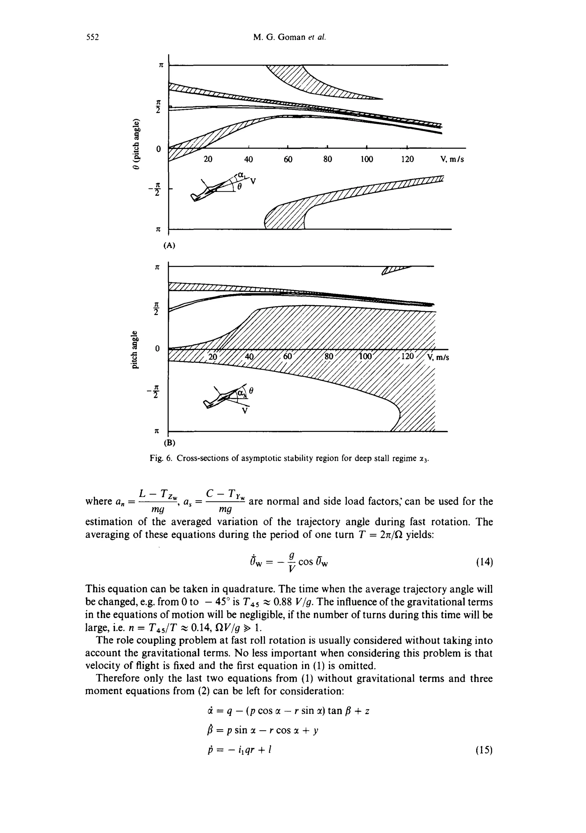
The region of attraction of critical deep stall regime in the general case will be more
complicated with respect to the region, considered above in simplified manner. To take into
account the interaction between phugoid and angular modes the first four equation of (10),
which are the autonomous nonlinear system with state vector X = (V, 0, ~, q)r, have to be
considered with entire ranges of .~ and 0 variations--I- ~t,n]. To represent the stability
region in the fourth-order state space it is possible only by means of drawing its two-
dimensional cross-sections considering the disturbances only in two selected state variables.](https://image.slidesharecdn.com/1997gomanzagainovkhramtsovsky-applicationofbifurcationmethodstononlinearflightdynamicsproblems-131005035700-phpapp01/75/1997-12-2048.jpg)


![Bifurcation methods in nonlinear flight dynamics 559
4O
0
•~ 30
o 20
m
t::
== 10
"6
--~ 0
t'-
< -10
O
0.5"10
2
g 0
2
• -0.5
>-
-1
-20 0 20
(A) Sideslip, dog
4
O
2
=-o
2_ 2
0
n'_ 4
-6
(B)
10
O
s
'lO
=- 0
2
o -5
fie
-10
-20 0 20 40
-20 0 20 40
Sideslip, deg
.....~ ' 7 ' _ .....
.. : , ~
i
-20 0 20
(C) Sideslip, dog (D) Aileron deflection, deg
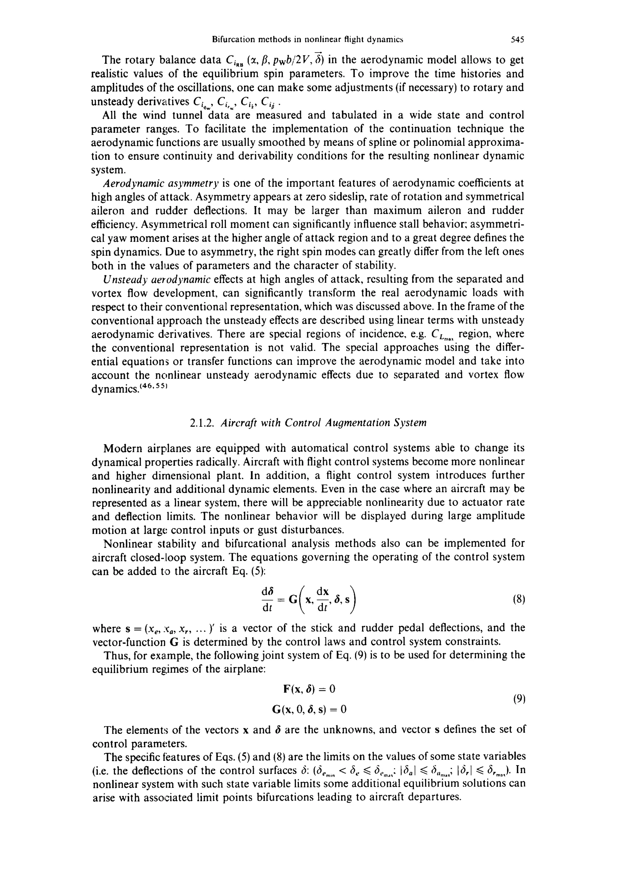
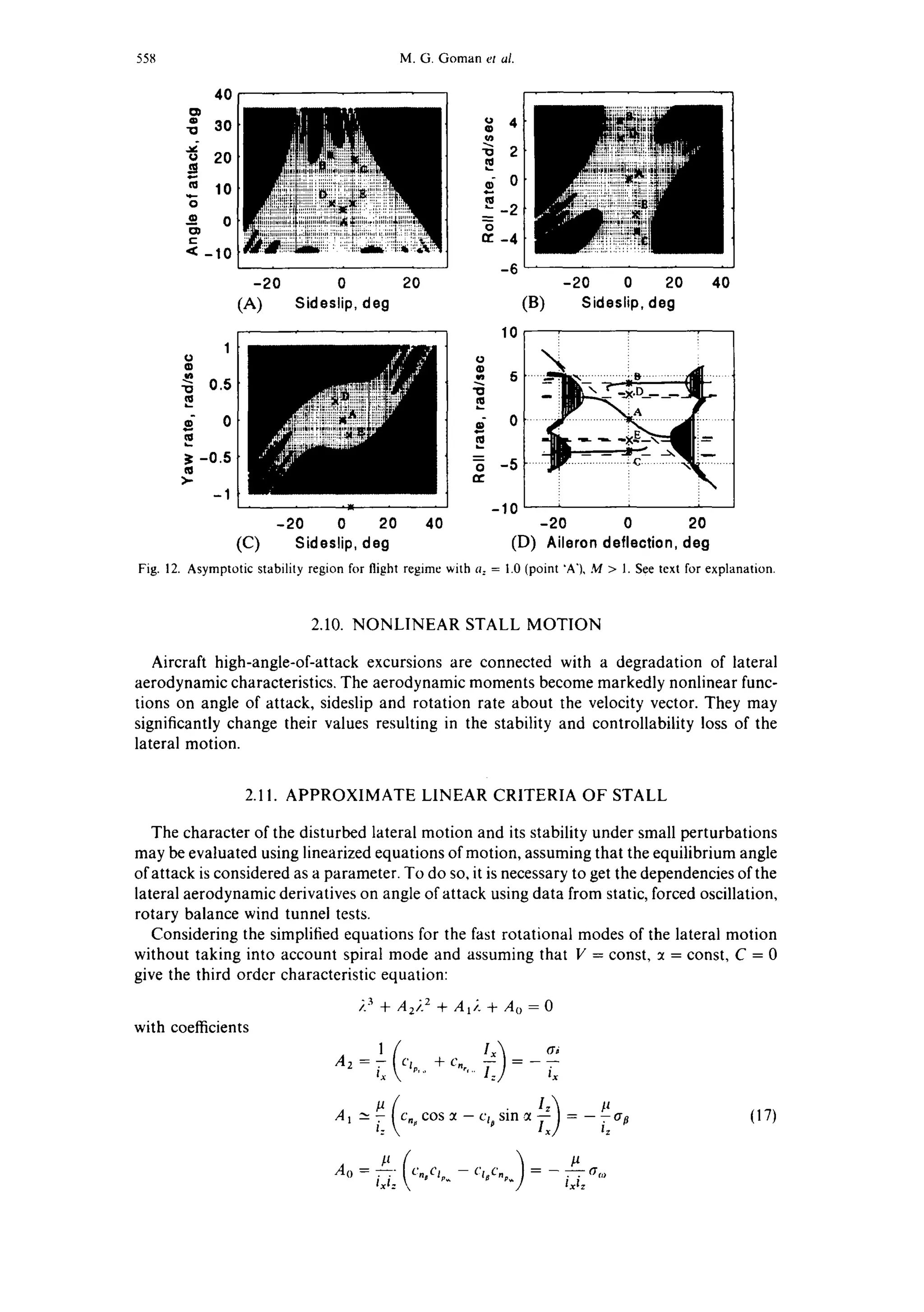
Fig. 13. Asymptotic stability region for flight regime with a= = 0.0 (point 'A'), M > 1. See text for explanation.
40
0
'1o 3O
o 20¢1
== 10
0
• 0
C
-10
1O
O
0.5"ID
d 0
~ -0.5
m
-1
-20 0 20
(A) Sideslip, deg
-20 0 20
(C) Sideslip, deg
~ 4
"~ 2
¢- 0
~-2
0
~-4
-6
10
0
0
~ -S
-10
40
,,~~h'):]t;
-20 0 20
(B) Sideslip, deg
40
5 ...... . . ~ B . ..................:...--......
-20 0 20
(D) Aileron deflection, dog
Fig. 14. Asymptotic stability region for flight regime with a: = - 1.0 (point 'A'), M > 1. See text for explanation.](https://image.slidesharecdn.com/1997gomanzagainovkhramtsovsky-applicationofbifurcationmethodstononlinearflightdynamicsproblems-131005035700-phpapp01/75/1997-21-2048.jpg)

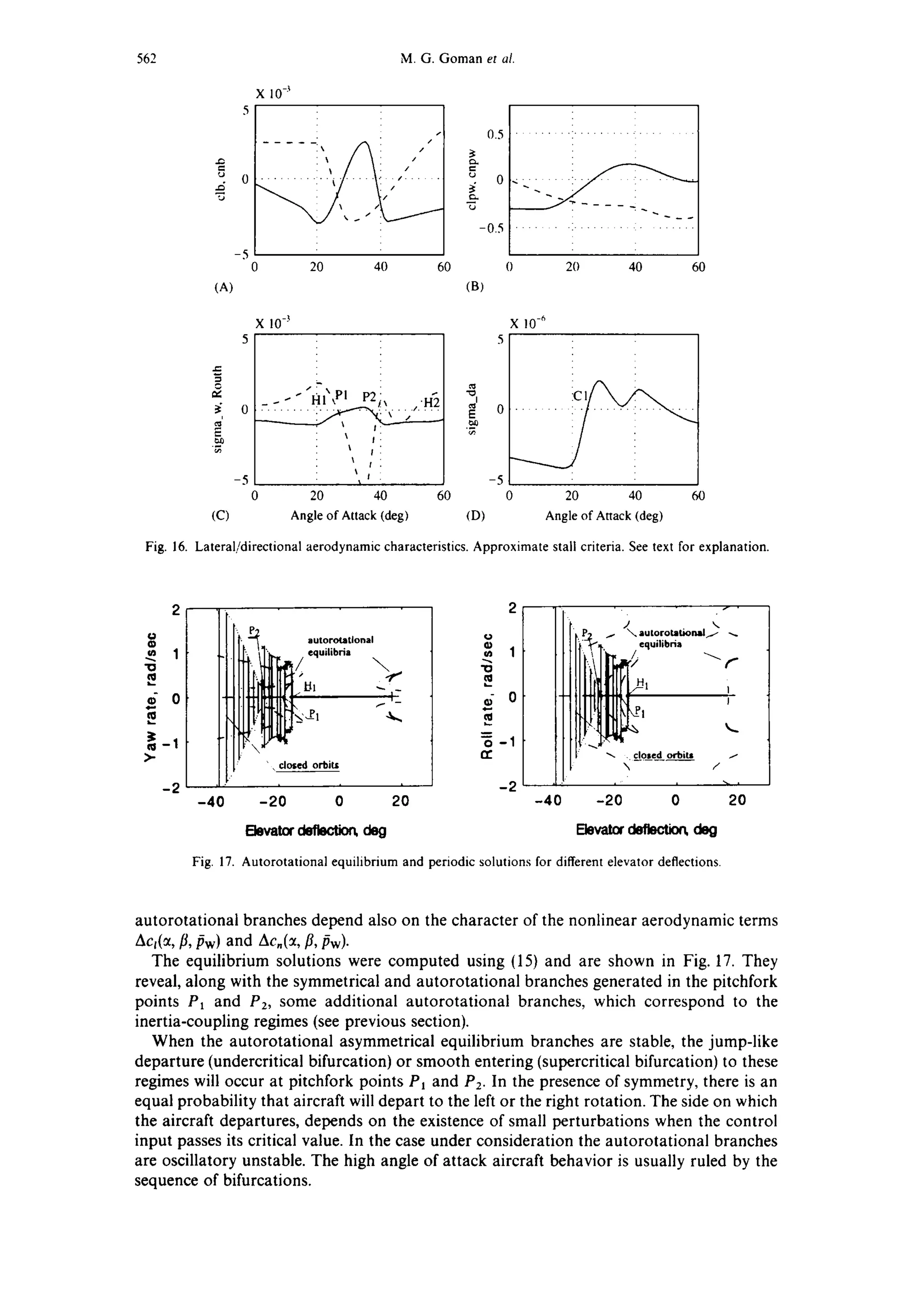
![Bifurcation mcthods in nonlinear flight dynamics 563
Winy Rock motion usually arises in the Hopf bifurcation point, which in our case is
preceded to the first pitchfork point. The Hopf bifurcation points Ht (at ~ ~ 2C) and H2
(at :t ~, 46°) generate the families of the stable closed orbits, which defines the wide range of
the wing rock motion.
In Fig. 17 the amplitudes of the asymmetrical closed orbits, calculated by means of
continuation, starting from point Hi, are presented by dark lines. Really the oscillatory
behavior is much complicated. In Fig. 18 the Poincar~ mapping, defined as the crossing
points of the plane p = 0, is presented for :t and/3 as a function of elevator deflection. The
crossing points at every given elevator deflection are taken after a very long time of
adjustment (t = 200s). Therefore, all the calculated results correspond to the stable solu-
tions. There are some ranges with symmetric periodic solutions with a single and doubled
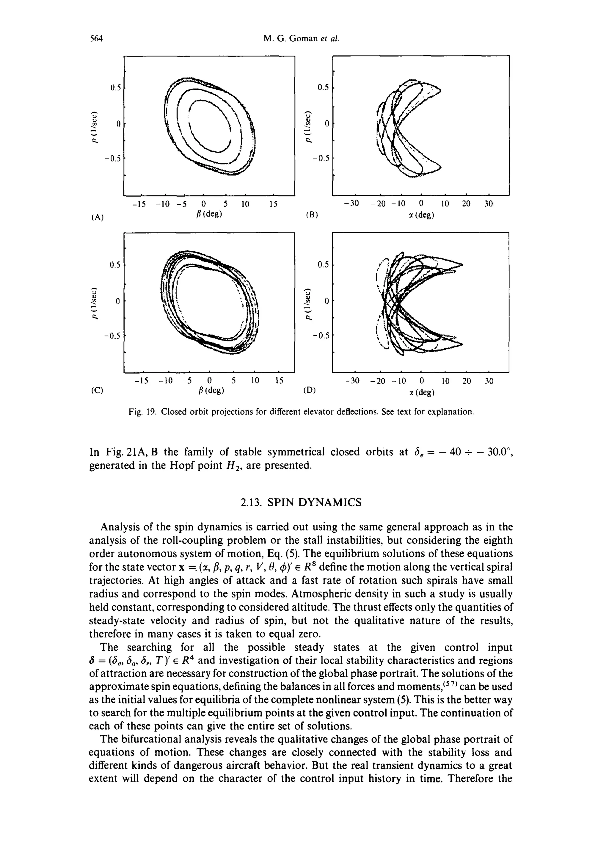
period. There is a narrow range (fie~ - IC) with chaotic motion. This regime arises from
the symmetrical periodic solutions after a sequence of bifurcations. First the symmetrical
stable closed orbits (see Fig. 19A, B) becomes unstable due to pitchfork bifurcation. After
that, both the unstable symmetrical and stable asymmetrical are subjected to the sequence
of flip bifurcations (see Fig. 19C, D) and as a result a strange attractor appears in accord-
ance with Feigenbaum scheme/~°~ To visualize this 'strange' attractor, four projections of
phase trajectory (p, fl),(p, ~t),(r, fl) and (r, :t), obtained by means of plotting only unconnec-
ted sequential points (20 dots per second), are presented in Fig. 20. Before chaotic behavior
simulation the long time adjustment was fulfilled (t = 2000 s).
Poincar~ mapping reveals also the wide regions with stable asymmetrical closed orbits
(see also Ref. 50). In such cases the aircraft will enter in the oscillatory wing-rock regime
applied on spiral motion.
The more complicated case of the periodic solutions is presented in Fig. 21C, D for
6~ =- 20.5 ~. There are three stable closed orbits (one of them symmetrical and two
asymmetrical) and two unstable closed orbits. In such a case, the final kind of motion will
depend on the initial conditions of state variables, i.e. on the prehistory of control.
40
30
20
(A)
I I I I I I I
-22 -20 -18 -16 - 14 -12 -10
fie (deg)
10
5
0
-5
-10
-15
chaoticmotion
-- ~ ] doubling
, , , ,, , , ,
-22 -20 - 8 - 6 -14 - 2 -I0
(B) 6~.(deg)
Fig. 18. Poincar6 mapping of p = 0 plane for different elevator deflections. See text for explanation.](https://image.slidesharecdn.com/1997gomanzagainovkhramtsovsky-applicationofbifurcationmethodstononlinearflightdynamicsproblems-131005035700-phpapp01/75/1997-25-2048.jpg)


![Bifurcation methods in nonlinear flight dynamics 571
20
-20
-40
"'1 13 [
/ 9 7 //1 7 1 9 ~x~
5 :'~
..... ~ ~; -..z.,.,.. 7 "~"'-~" ~ -- .....
I I I
-20 0 20
~. (deg)
Fig. 26. Bifurcational diagram of HIRM equilibria in the plane of elevator and aileron deflections. Eighth order
equations, no asymmetry, no thrust, ~t > 20°, 6c = 0, 6, = 0, H = 5 km.
100
80
60
40
20
0
-20
(A)
-,m...... ~pin,s
'-'"377'.'~] ..........................................................
WingRock~
/
-30 -25 -20 -15 -I0 -5 0 5 10 15 20
• o • .* .k
.......".:::.,~. ..."
80 - "w': ".................
Spi,~ f
60-
40 " WingRock ............
.:,,..; ....... ---"..:::.,..,~::::............. ..
• , 4,,, -. :
20- .......... _ 1 ..........
6, =-10.19"
0
-70
(B) ~,
-50 -30 -10 10 30 50 70
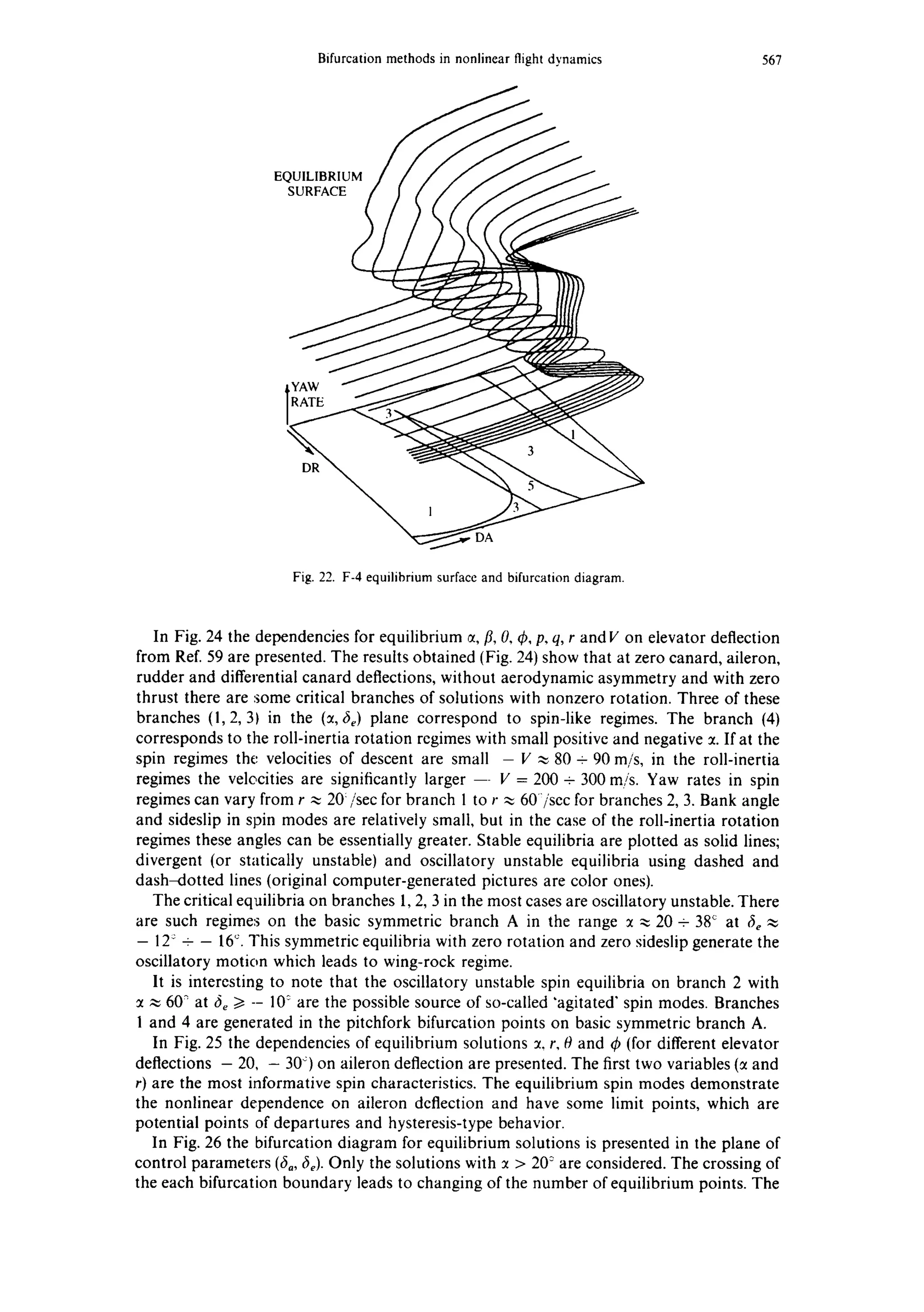
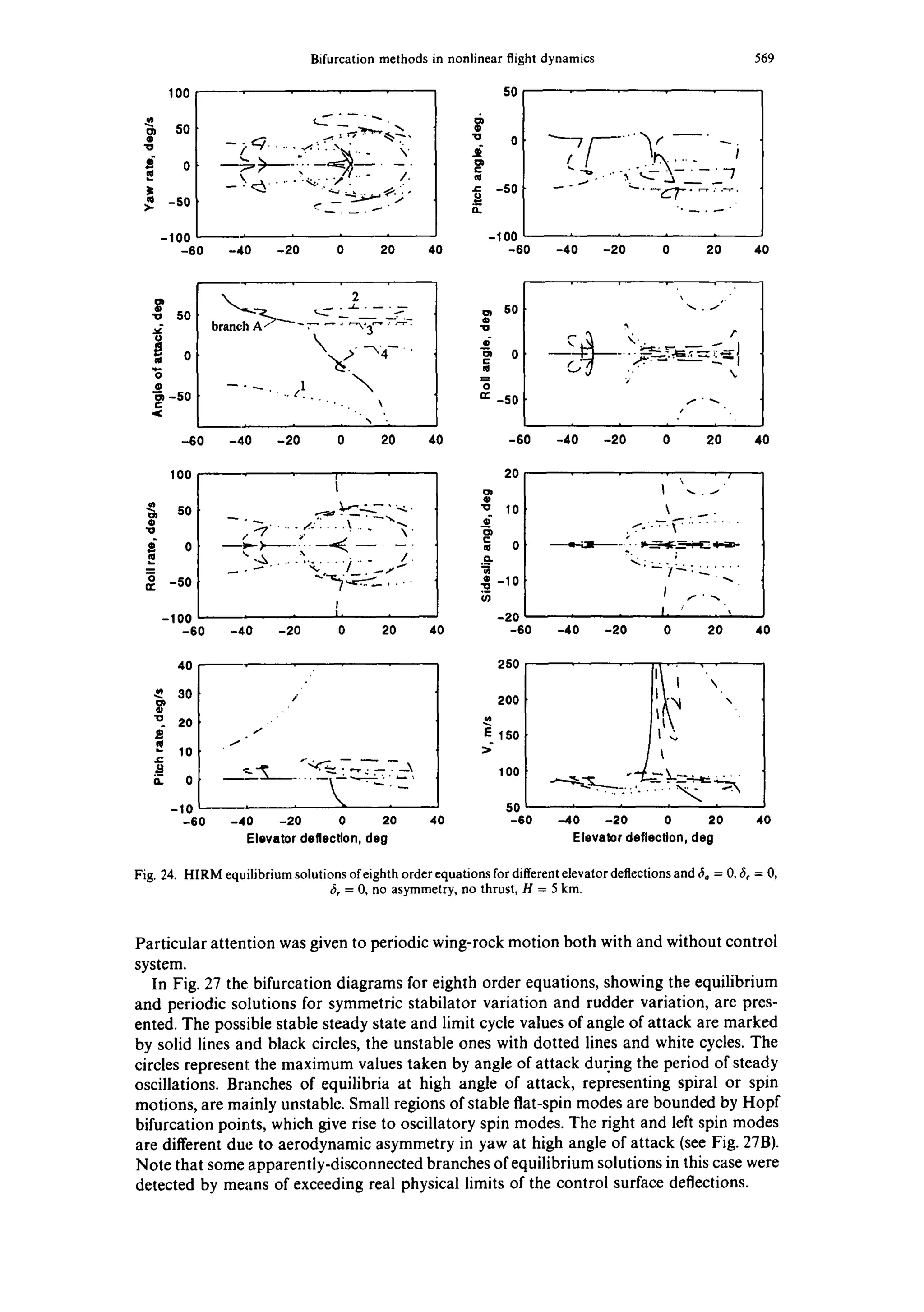
Fig. 27. F-15 equilibrium and periodic solutions of eighth order equations of motion; A) symmetric stabilator
variation, 6, = 0; B~ rudder variation, fie = - 12.2°. Bifurcation diagram for equilibrium and periodic solutions.
36 30 •
32
28
24
20
16
-1.5
-'28.1
-1.0 -0.5 0.0 0.5 1.0 1.5 6
(A) P (a)
28 - 21.2 22 2
~ 26 • 20.2 "~s 22.1
18.9 ~
24. 18.1
17.6
Flong= 17.2
22
-6 -4 -2 0 2 4
Fig. 28. F-15 wing-rock motion. Periodic orbit projections for varying longitudinal parameter; A) orbits for
open-loop system, B) orbits for closed-loop system.
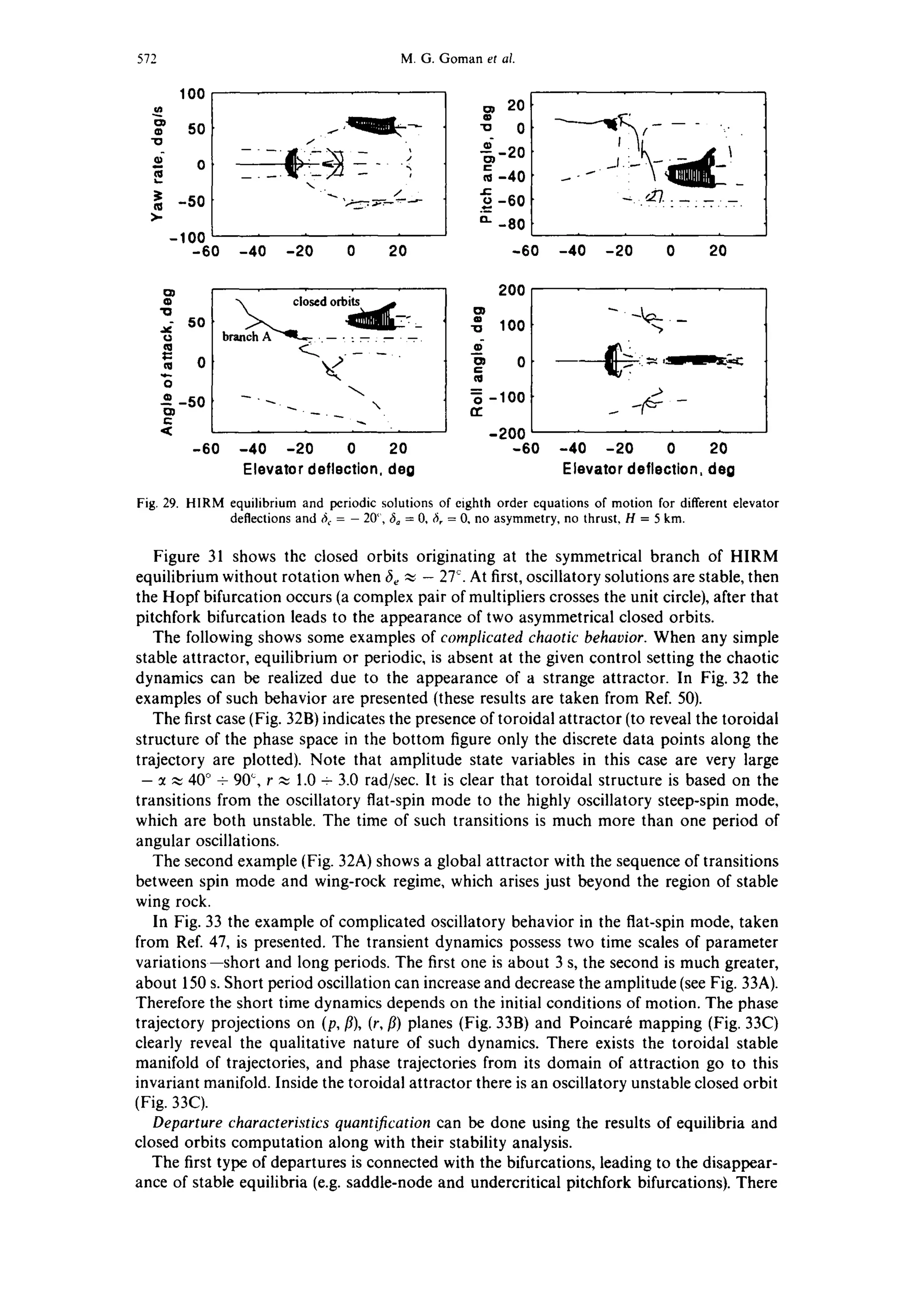
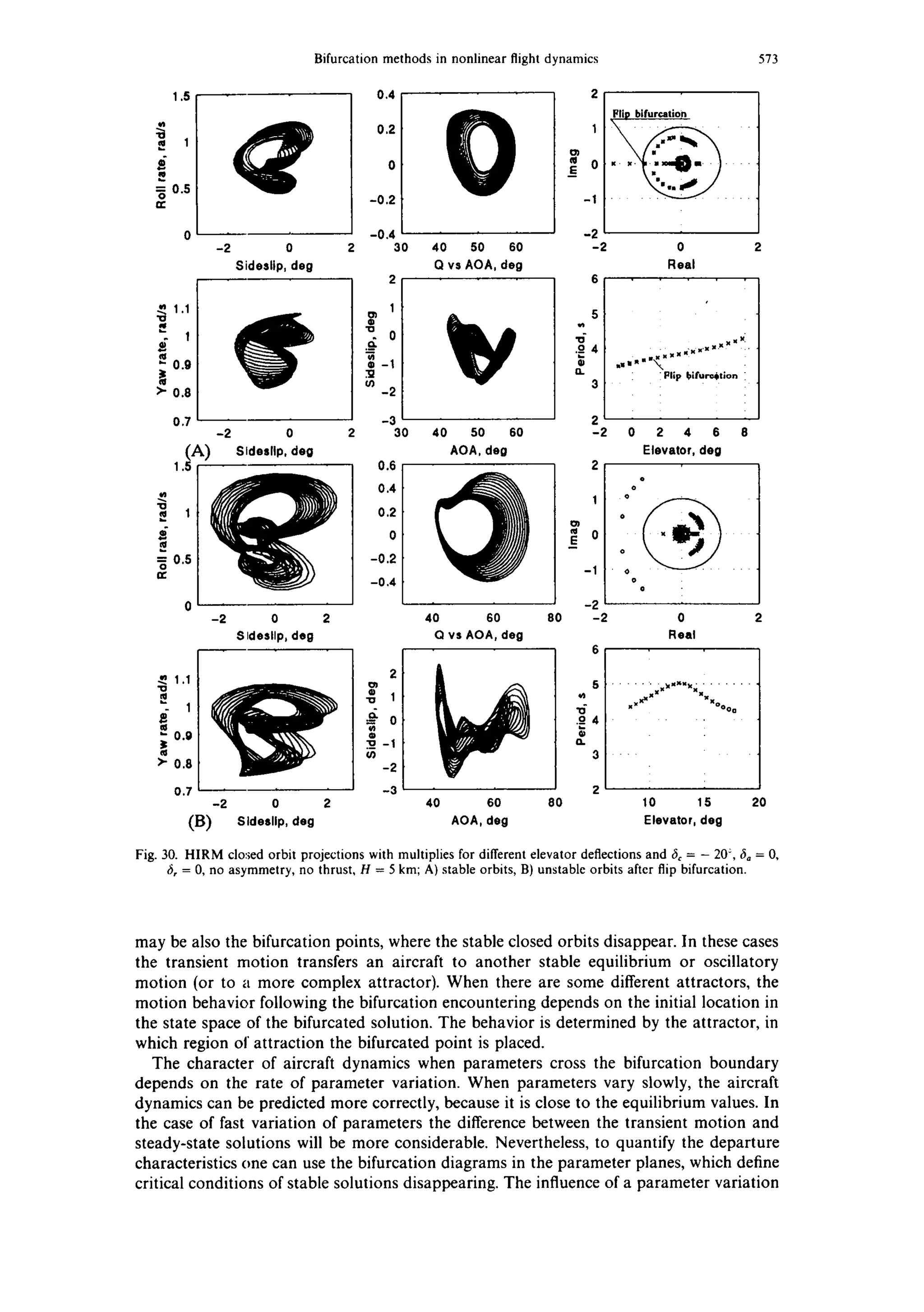
when their amplitudes are relatively small at fie ~ - 2° - 2° (see Fig. 30A). At 6e > 2° the
closed orbits become unstable (see Fig. 30B) after the flip or period doubling bifurcation
arises. As one can see in Fig. 29, the amplitudes in pitch (Act, A0) of single-period closed
orbits are much larger than the amplitudes in the lateral motion (Ar, Ap, A~, Aft).](https://image.slidesharecdn.com/1997gomanzagainovkhramtsovsky-applicationofbifurcationmethodstononlinearflightdynamicsproblems-131005035700-phpapp01/75/1997-33-2048.jpg)

![Bifurcation methods in nonlinear flight dynamics 577
¢=
'10
=-
all
]=
¢l
>.
100 - -
50
0
-50
-100 - -
-60 -40 -20 0 20 40
0 -- -
nl
-so
-100
-60 -40 -20 0 20 40
0
-v 50
~ 0
o
o
-50e-
branch 2
branch A
-60 -40 -20 0 20
100
5O
"o
" 0r-
eO
~- -50
-100
40 -60 -40 -20 0 20 40
100
} so
$ 0
~ -50
-100 L
-60
_ -
-~i' / /
, ~ ,
-40 -20 0 20
k
2O
ii0Io-10
-20
40 -60 -40 -20 0 20 40
et
o
"o
°
m
J~
0.
40
30
20
10
0
-10
-60
$ /
<P
** / t
iI" oo • • o-o- ~
-40 -20 0 20
Elevator deflection, deg
250
200
E 150
100
I
L
I -
50
40 -60 -40 -20 0 20 40
Elevator deflection, deg
d3~
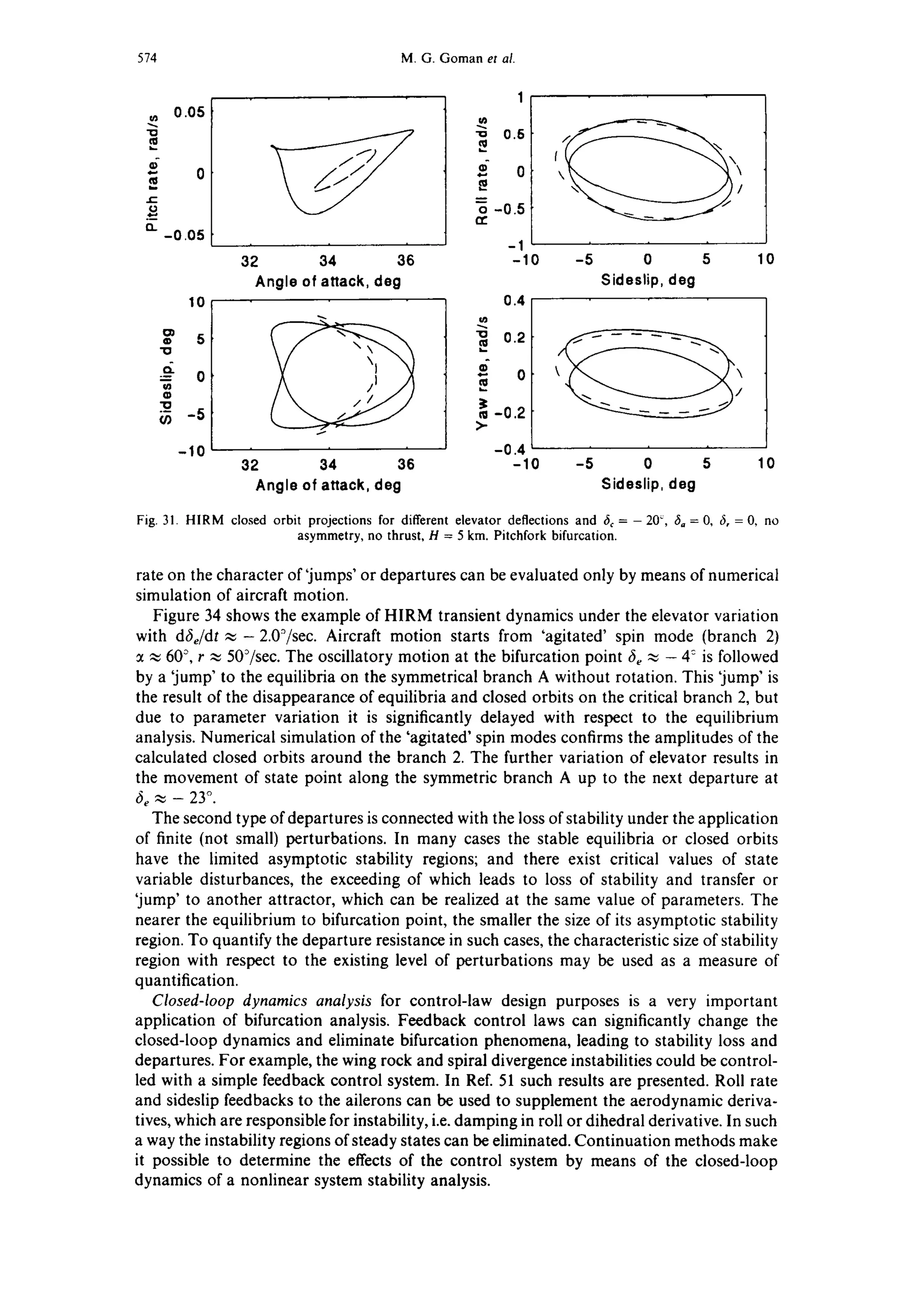
Fig. 34. Transient H1RM dynamics under elevator variation with ~- ~ - 2.0~/sec in comparison with equilib-
rium solutions (3, = - 20', 30 = 3, = 0, H = 5 km).
where F is a smooth vector function. The vector field F defines a map R"÷" ---,R'. The
system (20) satisfies the conditions of the existence and uniqueness of solutions x(t, Xo) with
initial condition x(0, Xo) = Xo. The solution curve ~o,(Xo)= x(t, Xo) is called the trajectory
and together wtth other trajectories forms the flow of the dynamical system. The set of all
trajectories constitute the phase portrait of the dynamical system.
The concept of the critical elements of a nonlinear autonomous dynamical system is the
basic one. The critical elements are invariant manifolds of trajectories, the dimensions of
which vary from 0 up to n - 1. The simplest ones are well-known equilibrium points or
zeroes of a vector field and closed orbits, which define the periodic solutions. They may be
attractive for other trajectories, if they are stable. There are also more complex attractors in
high order dynamical system (n/> 3). For example, invariant toroidal manifolds of trajecto-
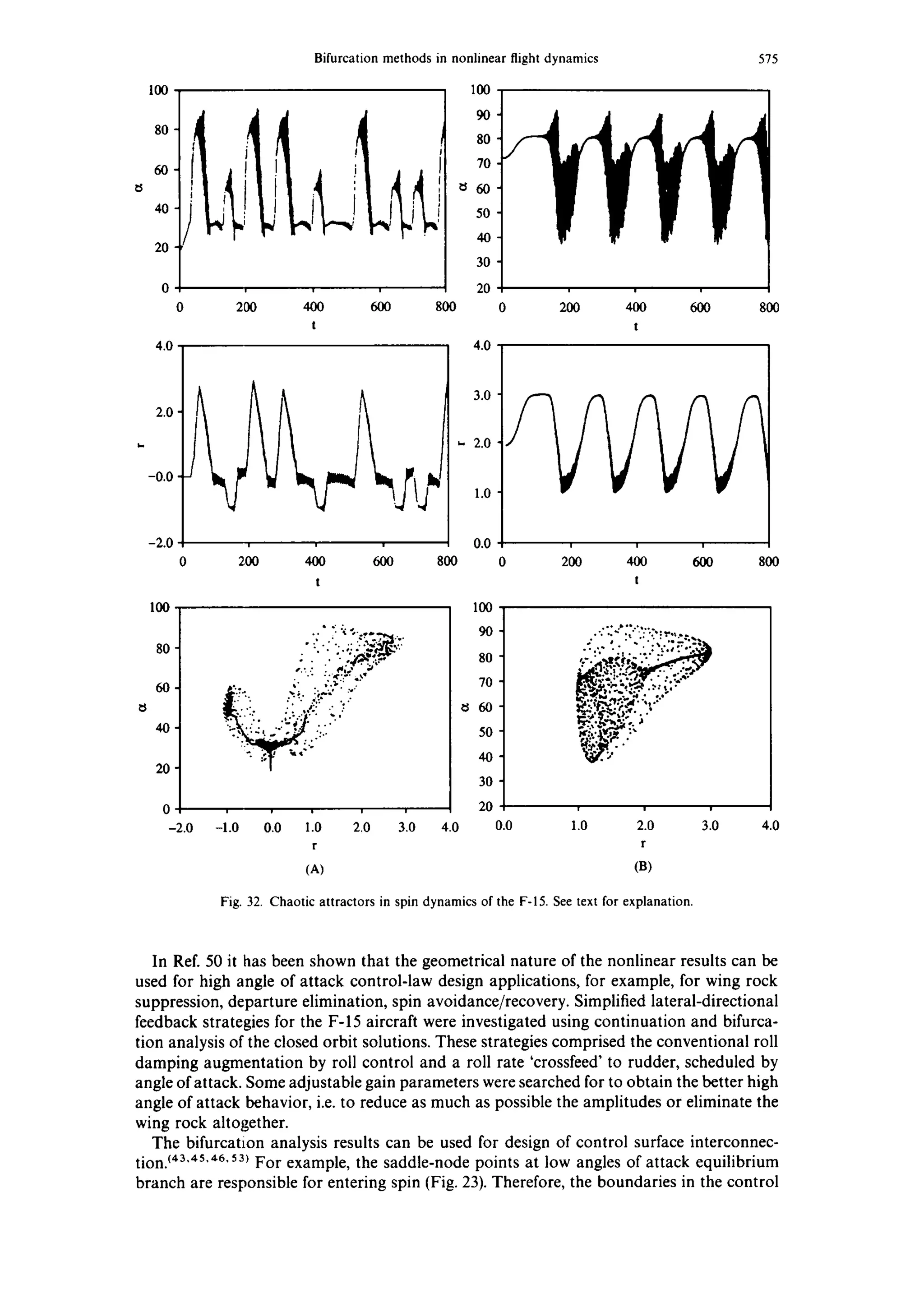
ries and 'strange' attractors (see Fig. 35).](https://image.slidesharecdn.com/1997gomanzagainovkhramtsovsky-applicationofbifurcationmethodstononlinearflightdynamicsproblems-131005035700-phpapp01/75/1997-39-2048.jpg)

![582 M.G. Goman et al.
ImZ.
Rek
0 ~"
Saddle-nodebifurcation
/~.... limitpoint(det~x_=.0_)
I
supercriticafl
branching point
undercrilical
/ g
transcritical
~,$/S"
/
/
Andronov-Hopfbifurcation
o~o Rek
~] - supereritieal
Fig. 39. Bifurcations of the equilibrium points.
subcritical case, when two mirror-symmetrical stable or unstable limit cycles are
created or disappear.
• Multiplier crosses the unit circle at the point (-1, 0) the stable closed orbit becomes
unstable and stable periodic orbit with doubled period detaches from the initial closed
orbit. This bifurcation is called flip or period doubling bifurcation; usually the period
doubling bifurcations appear in the form of so-called Feigenbaum cascade, leading to
chaotic motion.
• A pair of multipliers crosses the unit circle at the points e -+'~, the closed orbit becomes
oscillatory unstable while the stable two-dimensional toroidal manifold appears; there
are also supercritical and undercritical types of such bifurcation.
There are also other situations when closed orbits disappear:
• The periodic trajectory F shrinks into a point.
• An equilibrium point emerges on the closed orbit F.
• Some point belonging to F goes to infinity, thus the curve is no more closed.
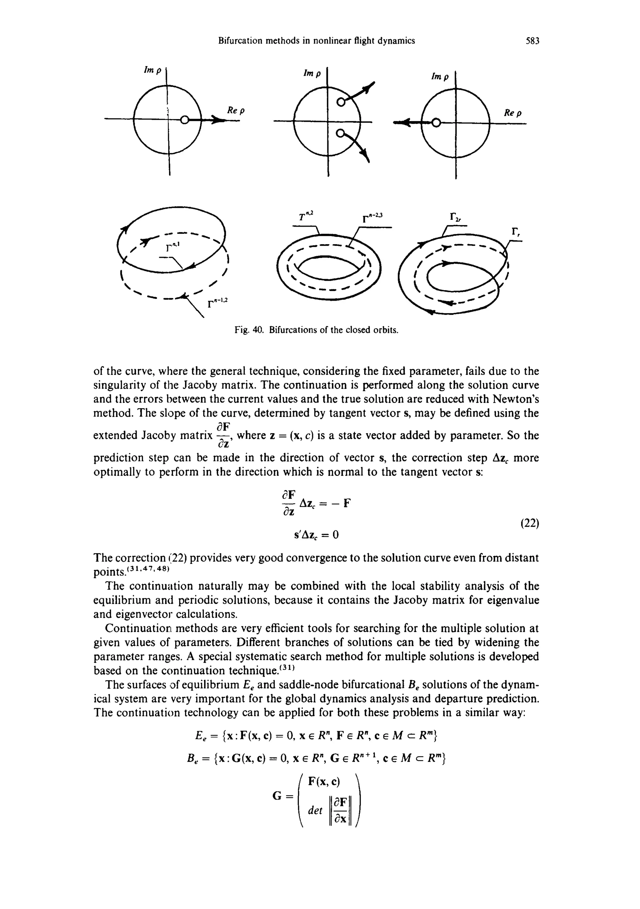
Continuation methods are widely applied for computer-aided qualitative analysis of
dynamical systems in many general-purpose and specialized for different applications
Packages.(19'2°'22'31) There are several versions of continuation algorithms for solving
the nonlinear problems (e.g., searching for equilibrium solutions -- F(xe, e) = 0, or fixed
points of Poincar6 mapping--P(x,) = x,). The main feature of these algorithms is the
introduction a general arclength for the solution curve in the extended by parameter state
space. Such consideration permits one to overcome the singular problem in the limit points](https://image.slidesharecdn.com/1997gomanzagainovkhramtsovsky-applicationofbifurcationmethodstononlinearflightdynamicsproblems-131005035700-phpapp01/75/1997-44-2048.jpg)


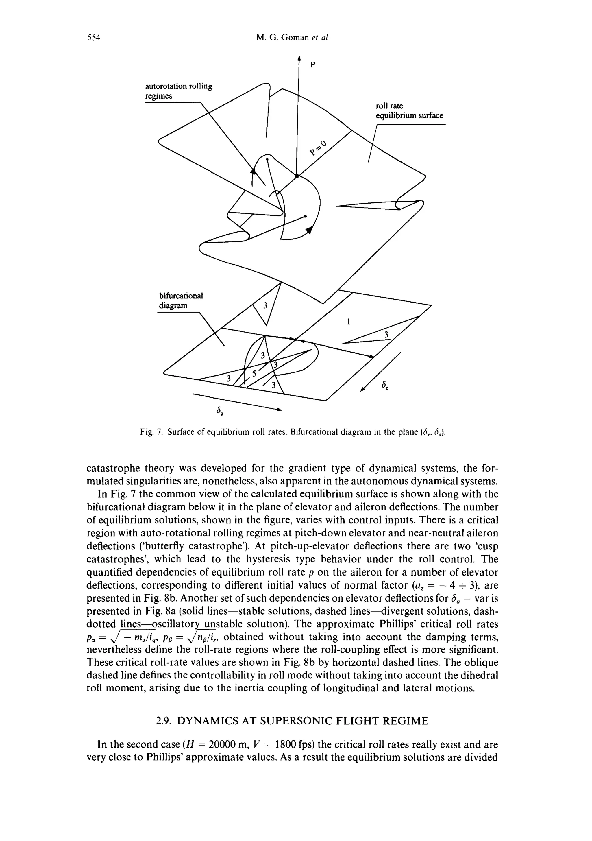
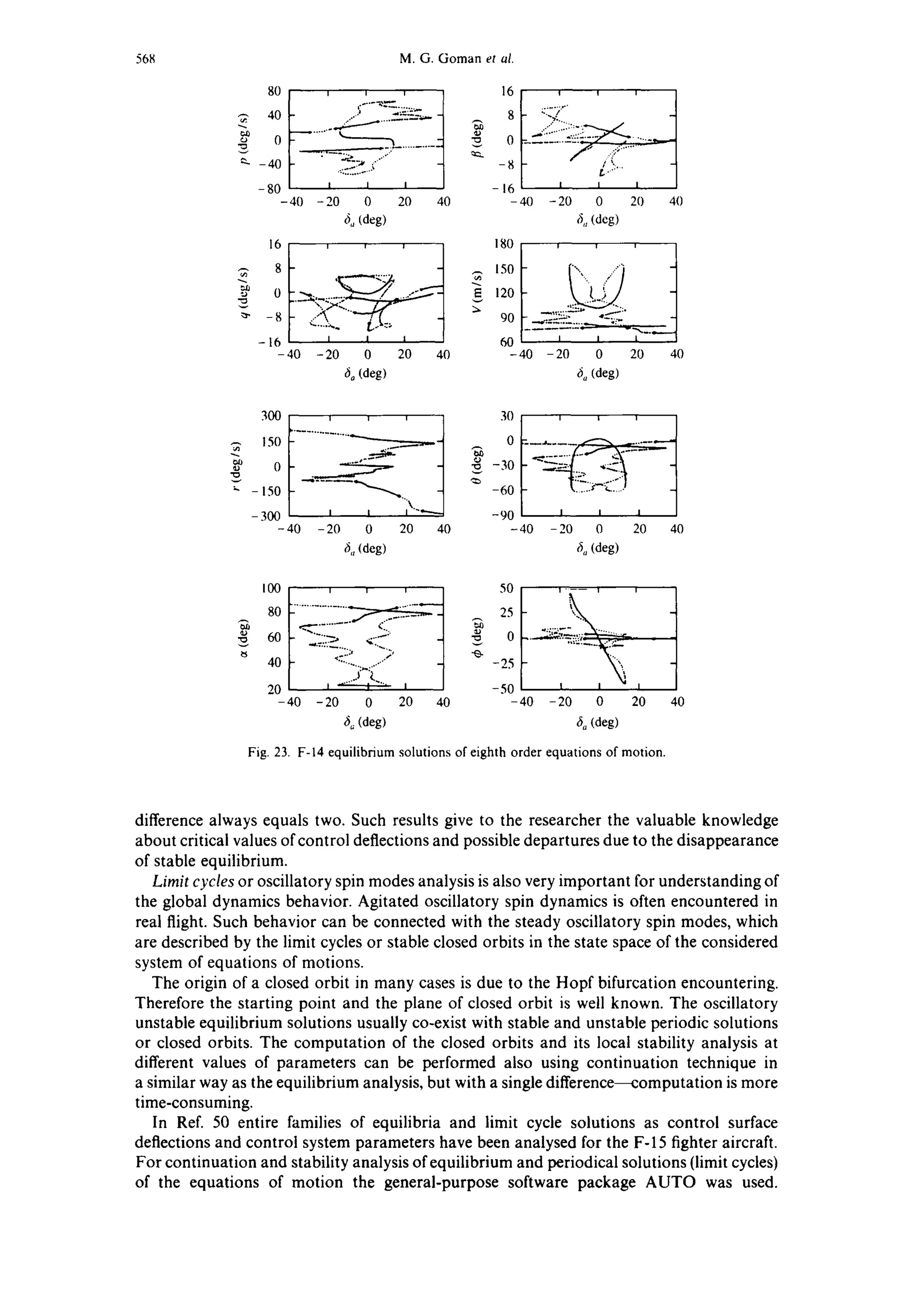
This document discusses the application of bifurcation methods to analyze nonlinear problems in flight dynamics, such as stall, spin, and roll-coupling. It provides an overview of how bifurcation analysis and continuation techniques have been used to study these problems for various aircraft, including the F-4, F-14, and F-15. The document outlines the methodology for applying bifurcation analysis, which involves using continuation methods to find equilibrium solutions and closed orbits, analyzing their stability, and predicting behavior as parameters vary. This allows researchers to better understand nonlinear aircraft dynamics at high angles of attack and critical flight regimes.