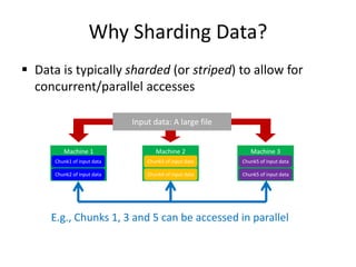
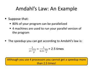
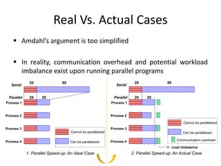
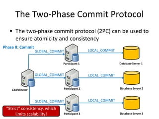
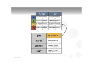
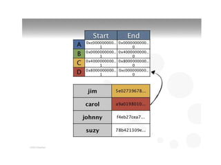
This document discusses different types of databases including NoSQL databases. It describes four types of data: structured, unstructured, dynamic, and static. It then discusses scaling traditional relational databases vertically and horizontally. It introduces the concepts of data sharding, Amdahl's law, and data replication. The challenges of consistency in replicated databases and solutions like two-phase commit are covered. The CAP theorem and eventual consistency are explained. Finally, different types of NoSQL databases are classified including document stores, graph databases, key-value stores, and columnar databases. Specific NoSQL databases like MongoDB, Neo4j, DynamoDB, HBase, and Cassandra are also overviewed.
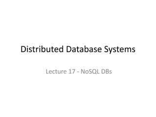
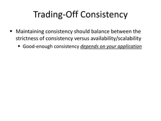

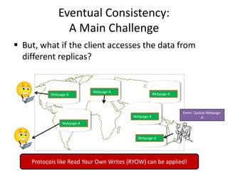
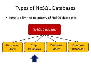
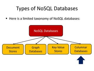
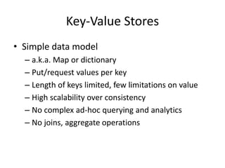
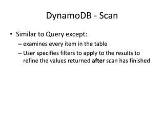
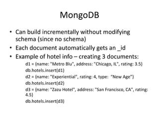
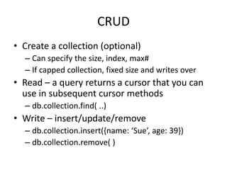
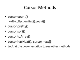
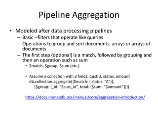
![HBase
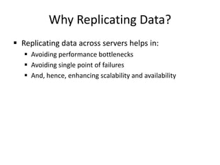
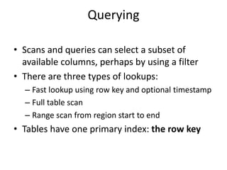
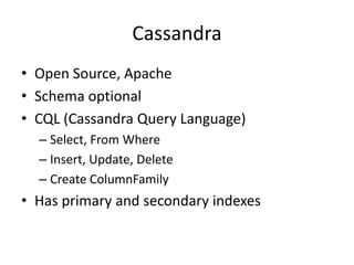
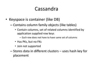
• Tables are sorted by Row Key
• Table schema only defines its column families .
– Each family consists of any number of columns
– Each column consists of any number of versions
– Columns only exist when inserted, NULLs are free.
– Columns within a family are sorted and stored
together
• Everything except table names are byte[]
• (Row, Family: Column, Timestamp) Value](https://image.slidesharecdn.com/17-nosql-230113072816-d9cb55b8/85/17-NoSQL-pptx-42-320.jpg)
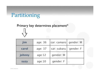
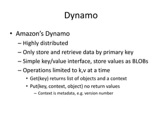
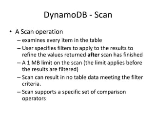
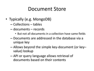
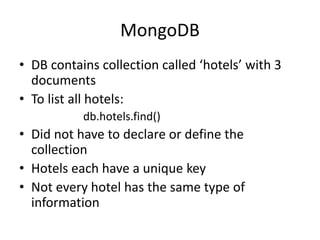
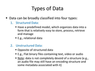
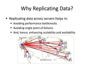
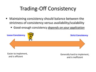
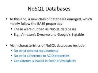
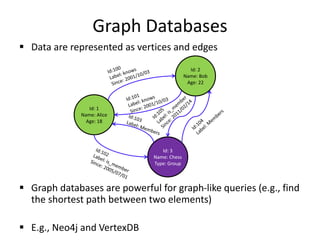
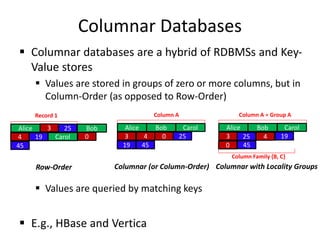
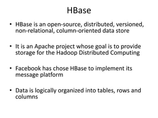
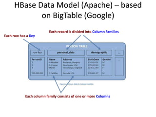
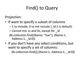
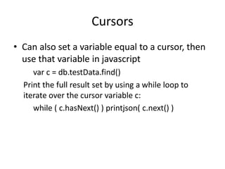
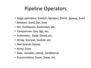
![Data types
• A field in Mongodb can be any BSON data type
including:
– Nested documents
– Arrays
– Arrays of documents
{
name: {first: “Sue”, last: “Sky”},
age: 39,
classes: [“database”, “cloud”]
}](https://image.slidesharecdn.com/17-nosql-230113072816-d9cb55b8/85/17-NoSQL-pptx-68-320.jpg)
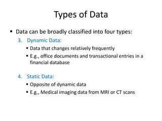
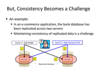
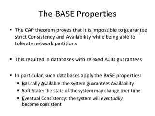
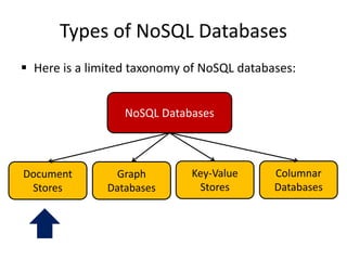
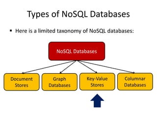
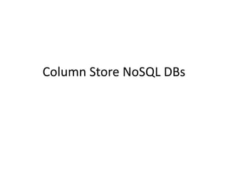
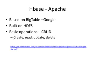
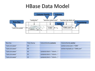
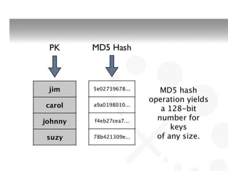
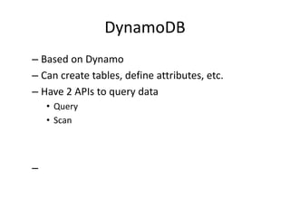
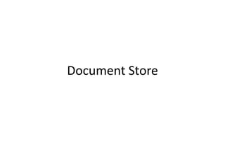
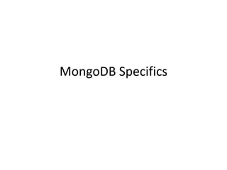
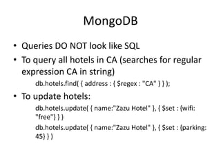
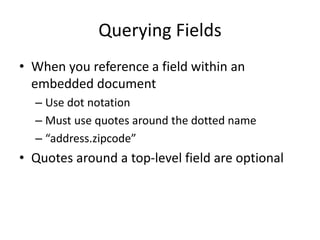
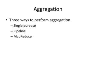
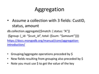
![Find() to Query
db.collection.find(<criteria>, <projection>)
db.collection.find{{select conditions}, {project columns})
Select conditions:
• To match the value of a field:
db.collection.find({c1: 5})
• Everything for select ops must be inside of { }
• Can use other comparators, e.g. $gt, $lt, $regex, etc.
db.collection.find ({c1: {$gt: 5}})
• If have more than one condition, need to connect with
$and or $or and place inside brackets []
db.collection.find({$and: [{c1: {$gt: 5}}, {c2: {$lt: 2}}] })](https://image.slidesharecdn.com/17-nosql-230113072816-d9cb55b8/85/17-NoSQL-pptx-69-320.jpg)
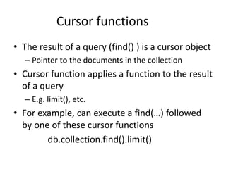
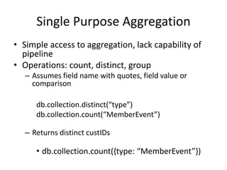
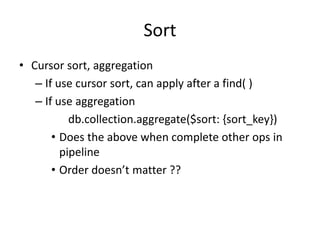
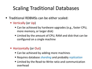
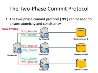
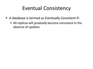
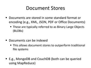
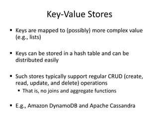
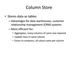
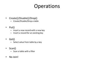
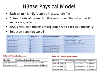
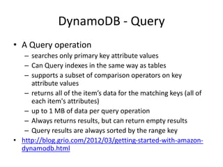
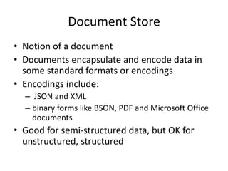
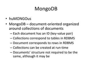
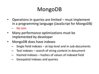
![Arrays
• Arrays are denoted with [ ]
• Some fields can contain arrays
• Using a find to query a field that contains an
array
• If a field contains an array and your query has multiple conditional
operators, the field as a whole will match if either a single array element
meets the conditions or a combination of array elements meet the
conditions.](https://image.slidesharecdn.com/17-nosql-230113072816-d9cb55b8/85/17-NoSQL-pptx-81-320.jpg)