SlideShare a Scribd company logo
1 of 32
Download to read offline
Research Article
Journal of Advanced Research in Economics and Business Management
Copyright (c) 2021: Author(s). Published by: Advanced Research Publications
Journal of Advanced Research in Economics and Business Management
Volume 4, Issue 2 - 2021, Pg. No.4-35
Peer Reviewed Journal
I N F O A B S T R A C T
Corresponding Author:
Bhadrappa Haralayya, Department of MBA
Lingaraj APPA Engineering College Bidar.
E-mail Id:
bhadrappabhavimani@gmail.com
How to cite this article:
Haralayya B, Jeelan BV, Vibhute NS. Capital
Structure and Factors Affecting Capital Structure.
J Adv Res Eco Busi Mgmt 2021; 4(2): 4-35.
Date of Submission: 2021-12-13
Date of Acceptance: 2021-12-30
Capital Structure and Factors Affecting
Capital Structure
Bhadrappa Haralayya1
, Jeelan Basha V2
, Nitesh S Vibhute­3
1
HoD and Associate Professor, Department of MBA, Lingaraj APPA, Engineering College Bidar, Karnataka, India.
2
Dean and Professor of Commerce, Vijayanagara Sri Krishnadevaraya University, Bellary, Karnataka, India.
3
Assistant Professor, Faculty of Business Studies MBA, Sharnbasva University, Karnataka, India.
Capital structure decisions are perhaps one of the most important
decisions taken by financial managers. It is one of the important and
challenging issues in corporate finance. What should be the appropriate
mix of debt and equity in capital structure.
The answer to this question has been debated in different literatures
pertaining to capital structure by different researchers. The enormous
work in this area by different researchers has tried to investigate of
optimal capital structure exists or not, which will help in maximization
of the wealth of the shareholders. The optimal mix of debt and equity
in capital structure will help in maximization the returns for the
shareholders, while minimizing the cost of capital. Decisions relating
to optimal combination of debt and equity have always raised the
inquisitiveness of different researchers all over the globe.
Keywords: Capital Structure, Financial Leverage, Business Risk,
Tangibility, Profitability
Introduction
There are number of capital structure theories which have
been propagated and have guided the researchers across
the globe to do their research in this area. We have basically
focused our research paper on two theories namely-pecking
order theory and trade off theories. The pecking off theory
basically states that the firm resort to internal finances first
and then debt capital as external financing. If required,
the last option for a firm as source of external finance is
distributed as dividend to the equity shareholders. The
firm has an option not to distribute the entire profit as
dividend, but retain a part of it as retained earnings for
future growth and expansion. Thus, as pecking theory, if
the firm is in need of funds, then it will first resort to the
retained earnings as internal finance and then to debt and
equity as external finance. The figures 1 explain the sources
of funds as per the pecking order theory.
Retained earnings
(internal)
Debt (external)
Equity
(external)
1st
preferred sources
2nd
preferred
sources
last resort
Table 1.Sources of funds as per the pecking
order theory
As per pecking order theory, there is no existence of optimal
capital structure. Trade off theory basically emphasizes on
existence of optimal capital structure. This theory states
that the firm should make a detailed cost-benefit analysis
before including debt in the capital structure. As stated in
the earlier paragraph, one of the important advantages
of including debt component in capital structure is the
benefit of tax shield on the interest component of the
debt capital. However, one of the major disadvantages of
5
Haralayya B et al.
J. Adv. Res. Eco. Busi. Mgmt. 2021; 4(2)
including debt in capital structure is that the financial risk
increases because of the constant interest burden of the
debt component. The finance manager should investigate
the pros and cons of including debt component in the
capital structure. Thus, an optimal capital structure can be
achieved with an appropriate mixture of equity and debt
in the capital structure so as to minimize the cost as well
as maximize the returns.
Our research paper has tried to investigate what deter-
minants the capital structure of a firm during the
recessionary period comprising of the pre and post period. It
is very important to understand the determinants of capital
structure before taking various crucial decisions related to
capital structure in an organization. When we were scanning
the different past literatures related to capital structure, it
was observed that the determinants of capital structure
different from one industry to the other.
For example: the capital structure determinants for the
textile industry differ from steel and cement industry. Thus
we decided to take BSE30 for our research taking a cross
section of different industries. It was prudent to take BSE30
for our research as the index represents 94% of the market
capitalization of the BOMBAY STOCK EXCHANGE, which is a
major and oldest stock exchange of INDIA. The index also
covers all the 7 major industries of INDIA namely private
and public banks, pharmaceutical, information technology,
etc. Thus, we decided to take BSE30 for our study as it will
include cross section industries of major sectors in INDIA
rather than concentrating on one specific/ industries.
Our entire research work has been segregated into pre-
recession period and post -recession period. Pre-recession
period has been taken from 2010-11 to 2014-2015 (total 5
years) and post-recession period is from 2015-16 to 2019-
2020 (total 5 years). Multiple regression analysis has been
utilized in this study to understand the capital structure
determinants for the firms which belong to BSE30 during
the pre as well as post recession period. The dependent
variable which has been taken in the study is “financial
leverage “ and 10 independent variables have been taken
as probable determinants of financial leverage or capital
structure during the pre and post period of recession.
Hence, the main purpose for conducting this study is to
investigate the determinants of capital structure or financial
leverage of BSE30 companies during the pre and post
recession period.
Objectives of the Study
The major objective of the research study focused on the
follows:
To identify those independent variables which are significant
determinants of capital structure (financial leverage) for
the firms belonging to BSE30 during the pre and post
recession period.
To rank the above significant variables determining the
financial leverage on the basis of their beta values.
To further investigate whether the variables significantly
determining the capital structure for BSE30 companies are
reflected pecking order or trade off theory during the pre
and post period of recession.
Research Methodology
Data Source
The present study was taken into consideration the
companies of BSE30. we derived a list of 30 companies
belonging to the BSE for the year spanning from 2009 -2010
to 2019 - 2020,which is segregated as prerecession period
from 2009-2010 to 2014-2015 and post recession period
from 2015-2016 to 2019-2020. Overall, 30 companies,
which satisfied all parameters, were utilized for the study.
Statistical Methods
Durbin Watson test has been used in this study to test
if the data are having time series influence or not. If the
data are stationary, then multiple recession analysis can
be done, otherwise we have to go for panel recession.
SPSS 20.0 software has been used to derive the correlation
matrix between the financial leverage (which is taken as
dependent variable) and the independent variables for both
the pre and post recession period. With the help of this
matrix, multi collinearity problem has been investigated.
The correlation between the independent variable should
be least for running multiple recession analysis. If the
correlation among the independent variable is very high,
then multicollinearity problem is assumed to exist and
we cannot continue with the multiple recession analysis.
High correlation has been defined in different researchers.
Lewis-beck (1980) stated that if the correlation between
the independent variables is equal to or more than. 80,
then multicollinearity problems will be assumed to exist.
This reference has been used in this research article. Thus,
thought correlation matrix, multi- collinearity problem has
been investigated and then multiple recessions have been
applied taking one dependent variable (financial leverage)
and 10 independent variables.
Variables taken in the study
Financial leverage is taken as a dependent variable in this
research paper. Financial leverage is defined as average total
assets divided by average total debt. Total debt includes
the sum total of both borrowings and currently liability and
provisions. It has been an endeavor in this study so as to
understand the determinants of financial leverage by taking
10 independent variables. The table 1 consists of the details
6
Haralayya B et al.
J. Adv. Res. Eco. Busi. Mgmt. 2021; 42)
regarding the dependent and the independent variables
taken for the study. The independent variable taken in the
study may have some impact on financial leverage.
Tangibility
Tangibility has been defined in this research paper as
average net fixed assets and average total assets. The trade
off theory assumes a positive relation between tangibility
and financial leverage.
Profitability
A return on assets has been taken as a proxy for profitability
inthispaper.Oneoftheimportantparametersformeasuring
the financial performance of a firm is by profitability. The
tradeoff theory indicates a positive relationship between
profitability and financial leverage. Pecking off theory,
which prefers internal financing to debt component as
source of finance, has profitability and financial leverage
are negatively related to each other.
Size of the firm
Some of the major studies in the past have indicated a
relation between size of the firm and financial leverage.
Trade off basically states a positive relationship between
size and financial leverage. A larger sized firm has better
debt bearing capacity, but pecking order theory emphasized
that size and financial leverage are negatively related to
each other. Two proxies have been used for “size of the
firm “in this research study, that is, log (total sales) and
log (total assets).
Interested coverage ratio: interest coverage ratio has been
defined in this project as the ration between average
earnings before interest and tax and average interest
paid. Positive relation between interest coverage ratio
and average financial leverage is supporting by the tradeoff
theory, but on the other hand, the pecking order theory
emphasizes that interest coverage ratio and financial
leverage are negatively related to each other.
Dividend Payout Ratio
Dividend payout ratio is defined as the ratio between
dividend and total income available to shareholders (profit
after tax). Here, dividend includes only dividend paid and
proposed. The tradeoff theory states that dividend payout
ratio and financial leverage are positively related to each
other.
Non Debt tax shield
Non debt tax shield has been defined in this article as
the ratio between the deprecation and total assets. It is
the tax deduction enjoyed by the business in the form
of deprecation. Tradeoff theory confirms a negative
relationship between financial leverage and non de bt
tax shield.
Degree of Operating Leverage
Increase in degree of opera-ting leverage in turn increases
thee fluctuation in the future profit earning. Operating
leverage and debt level in capital structure are negatively
related to each other. There is a greater chance that the
business failure will increase if the degree of operating
leverage increases. Hence, the organization will prefer
lesser debt in the capital structure. Both the pecking
order theory and tradeoff theory confirms a negatively
relationship between degree of operating leverage and
financial leverage.
Growth rate
Growthrateisanimportantdeterminantofcapitalstructure.
Pecking order theory confirms a positive relationship
between the growth rate (assets) and financial leverage.
It states that the highly growth oriented firms will prefer
more debt in their capital structure as their profitability
will allow them a cushion against the cost of debt. Thus,
if the growth opportunities are less, the organization will
prefer lesser debt in the capital structure and it will rely
more on internal financing. Trade off theory suggests a
negative relationship between growth rate (assets) and
financial leverage. If the growth opportunities increase,
the firm will prefer less leverage and retained more profit
in the business.
Business risk
One of the important variables in financial from dominant
knowledge s business risk. It is defined as the co efficient
of variables of earnings before interest and tax. With the
increases of business risk, the volatility of the earning will
also increase. Hence, the firm will prefer lesser debt in the
capital structure because of increased business risk. Thus,
the company will rely more internal financing rather than
debt a as source of financing. A negative relation is expected
between business risk and financial leverage.
Third Module
Concept of Capital Structure
The capital structure of a company is made up of debt and
equity securities that comprise a firm’s financing of its
assets. It is the permanent financing of a firm represented
by long-term debt, preferred stock and net worth. So it
relates to the arrangement of capital and excludes short-
term borrowings. It denotes some degree of permanency
as it excludes short-term sources of financing The relative
proportion of various sources of funds used in a business is
termed as financial structure. Capital structure is a part of
the financial structure and refers to the proportion of the
various long-term sources of financing. It is concerned with
making the array of the sources of the funds in a proper
manner, which is in relative magnitude and proportion.
7
Haralayya B et al.
J. Adv. Res. Eco. Busi. Mgmt. 2021; 4(2)
Category
Variable
code
Variable
name
Details
Dependent FL
Financial
leverage
Average total
debt/average
total assets
Independent FL
Interest
coverage
ratio
Average PBIT/
average interest
paid
Profit-
ability
Return on
assets
Average PBIT/
average total
assets
BR
Business
risk
Standard
deviation of
PBIT/average
PBIT
GR
Growth
rate
(assets)
Compound
growth rate of
total assets
DOL
Degree of
operating
leverage
% change in PBIT
to % change in
sales
Size_1
Size of the
firm (1)
Log (average
total sales)
Size_2
Size of the
firm (2)
Log(average total
assets)
TAN Tangibility
Average net fixed
assets/average
total assets
NDTS
Non debt
tax shield
Average
deprecation/
average total
assets
Meaning
The term capital structure refers to the percentage of
capital (money) at work in a business by type. Broadly
speaking, there are two forms of capital: equity capital
and debt capital.
Each type of capital has its benefits and drawbacks and
a substantial part of wise corporate stewardship and
management is attempting to find the perfect capital
structure regarding risk/reward payoff for shareholders.
This is true for Fortune 500 companies as well as small
business owners trying to determine how much of their
start-up money should come from a bank loan without
endangering the business.
Equity Capital 
Equity capital refers to money put up and owned by the
shareholders (owners). Typically, equity capital consists
of two types: 
•	 Contributed capital: The money that was originally
invested in the business in exchange for shares of
stock or ownership
•	 Retained earnings: Profits from past years that have
been kept by the company and used to strengthen
the balance sheet or fund growth, acquisitions, or
expansion
Many consider equity capital to be the most expensive
type of capital a company can use because its “cost” is
the return the firm must earn to attract investment. A
speculative mining company that is looking for silver in a
remote region of Africa may require a much higher return
on equity to get investors to purchase the stock than a
long-established firm such as Procter & Gamble, which
sells everything from toothpaste and shampoo to detergent
and beauty products.
Debt Capital
The debt capital in a company’s capital structure refers to
borrowed money that is at work in the business. The cost
depends on the health of the company’s balance sheet—a
triple AAA rated firm can borrow at extremely low rates vs.
a speculative company with tons of debt, which may have
to pay 15% or more in exchange for debt capital. There are
different varieties of debt capital:
•	 Long-term bonds: Generally considered the safest
type because the company has years, even decades,
to come up with the principal while paying interest
only in the meantime.
•	 Short-term commercial paper: Used by giants such as
Wal-Mart and General Electric, this amounts to billions
of dollars in 24-hour loans from the capital markets to
meet day-to-day working capital requirements such as
payroll and utility bills.
•	 Vendor financing: In this instance, a company can sell
goods before they have to pay the bill to the vendor.
This can drastically increase return on equity but costs
the company nothing. One secret to Sam Walton’s
success at Wal-Mart was selling Tide detergent before
having to pay the bill to Procter & Gamble, in effect,
using P&G’s money to grow his retail enterprise.
Table 2.List of dependent and independent
variables used in the study
DPR
Dividend
payout
ratio
Average
dividend/average
PAT (Profit after
Tax)
8
Haralayya B et al.
J. Adv. Res. Eco. Busi. Mgmt. 2021; 42)
•	 Policyholder“float”:Inthecaseofinsurancecompanies,
this is money that doesn’t belong to the firm but that
it gets to use and earn an investment on until it has to
pay it out for auto accidents or medical bills. The cost
of other forms of capital in the capital structure varies
greatly on a case-by-case basis and often comes down
to the talent and discipline of managers.
Capital Structure
A company’s capital structure points out how its assets
are financed. When a company finances its operations by
opening up or increasing capital to an investor (preferred
shares, common shares, or retained earnings), it avoids debt
risk, thus reducing the potential that it will go bankrupt.
Moreover, the owner may choose debt funding and
maintain control over the company, increasing returns on
the operations.
Debt takes the form of a corporate bond issue, long-term
loan, or short-term debt. The latter directly impacts the
working capital. Having said that, a company that is 70%
debt-financed and 30% equity-financed has a debt-to-equity
ratio of 70%; this is the leverage. It is very important for a
company to manage its debt and equity financing because
a favorable ratio will be attractive to potential investors in
the business.
From a technical perspective, the capital structure is defined
as the careful balance between equity and debt that a
business uses to finance its assets, day-to-day operations
and future growth.
From a tactical perspective however, it influences everything
from the firm’s risk profile, how easy it is to get funding,
how expensive that funding is, the return its investors
and lenders expect and its degree of insulation from
microeconomic business decisions and macroeconomic
downturns. By design, the capital structure reflects all of
the firm’s equity and debt obligations. It shows each type
of obligation as a slice of the stack. This stack is ranked by
increasing risk, increasing cost and decreasing priority in
a liquidation event (e.g., bankruptcy).
For large corporations, it typically consists of senior debt,
subordinated debt, hybrid securities, preferred equity and
common equity. Any company’s capital structure serves
several key purposes.
First and foremost, it’s effectively an overview of all the
claims that different players have on the business. The debt
owners hold these claims in the form of a lump sum of
cash owed to them (i.e., the principal) and accompanying
interest payments. The equity owners hold these claims
in the form of access to a certain percentage of that firm’s
future profit.
Secondly, it is heavily analyzed when determining how risky
it is to invest in a business and therefore, how expensive
the financing should be. Specifically, capital providers look
at the proportional weighting of different types of financing
used to fund that company’s operations.
For example, a higher percentage of debt in the capital
structure means increased fixed obligations. More fixed
obligations result in less operating buffer and greater
risk. And greater risk means higher financing costs to
compensate lenders for that risk (e.g., 14% interest rate
vs 11% interest rate).
Consequently, all else equal, getting additional funding
for a business with a debt-heavy capital structure is more
expensive than getting that same funding for a business
with an equity-heavy capital structure.
“Capital structure is essentially concerned with how the firm
decides to divide its cash flows into two broad components,
a fixed component that is earmarked to meet the obligations
toward debt capital and a residual component that belongs
to equity shareholders”-P. Chandra.
Definition - What does Capital Structure mean?
Capital structure refers to a company’s outstanding debt
and equity. It allows a firm to understand what kind of
funding the company uses to finance its overall activities
and growth. In other words, it shows the proportions of
senior debt, subordinated debt and equity (common or
preferred) in the funding. The purpose of capital structure is
to provide an overview of the level of the company’s risk. As
a rule of thumb, the higher the proportion of debt financing
a company has, the higher its exposure to risk will be.
Capital structure is commonly known as the debt-to-equity
ratio. Capital structure is the mix of the long term sources
of funds used by the firm. It is made up of debt and equity
securities and refers to permanent financing of a firm. It I
composed of long term debt, preference share capital and
shareholders fund.
“Capital structure is essentially concerned with how the firm
decides to divide its cash flows into two broad components,
a fixed component that is earmarked to meet the obligations
toward debt capital and a residual component that belongs
to equity shareholders”-P. Chandra.
“Capital structure of a company refers to the composition
or make up of its capitalization and it includes all long term
capital resources viz., loans, reserves, shares and bonds”
Gerstenberg.
Capital structure as, “balancing the array of funds sources
in a proper manner, i.e. in relative magnitude or in
proportions”- Keown et al.
Hence capital structure implies the composition of funds
raised from various sources broadly classified as debt and
equity. It may be defined as the proportion of debt and
9
Haralayya B et al.
J. Adv. Res. Eco. Busi. Mgmt. 2021; 4(2)
equity in the total capital that will remain invested in a
business over a long period of time. Capital structure is
concerned with the quantitative aspect. A decision about
the proportion among these types of securities refers to
the capital structure decision of an enterprise.
Importance of the Capital Structure	
Decisions relating to financial the assets of a firm are very
crucial in every business and the financial managers is often
caught in the dilemma of what the optimum proportion of
debt and equity should be. As a general rule there should
be a proper mix of debt and equity capital in financing the
firm’s assets. Capital structure is usually designed to serve
the interest of the equity shareholders.
Description
Value maximization: capital structure maximizes the market
value of a firm, i.e in a firm having a properly designed
capital structure the aggregate value of the claims and
ownership interests of the shareholders are maximized.
Cost minimization
Capital structure minimizes the firm’s cost of capital or cost
of financing. By determining a proper mix of funds sources,
a firm can keep the overall cost of capital to the lowest.
Increase in share price: capital structure maximizes the
company’s market price of share by increasing earnings
per share of the ordinary shareholders. It also increases
dividend receipt of the shareholders.
Investment opportunity
Capital structure increases the ability of the company to
find new wealth-creating investment opportunities. With
proper capital gearing, it also increases the confidence of
suppliers of debt.
Growth of the country
capital structure increases the country’s rate of investment
and growth by increasing the firm’s opportunities to engage
in future- creating investment.
Increases in value of the firm
A sound capital structure of a company helps to increases
the market price of shares and securities which, in turn,
lead to increase in the value of the firm.
Utilization of available funds
A good capital structure enables a business enterprise to
utilize the available funds fully. Properly designed capital
structures ensure the determinants’ of the financial
requirements’ of the firm and raise the firm.
Maximization of available funds
A sound capital structure enables management you increase
the profits of a company in the form of higher return to the
equity shareholders i.e. increasing in earning per share. It
can be done by mechanism of trading on equity.
Minimization of cost of control
A sound structure of any business enterprises maximizes
shareholders’ wealth through minimization of the overall
cost of capital. This can also be done by incorporation
long-term debt capital in the capital structure as the cost
of debt capitals lower than the cost of equity or preference
share capital since the interest on debt is tax deductable.
Solvency or liquidity position
It never allows a business enterprise to go for too much
rising of debt capital because, at the time of poor earning,
the solvency is distributed for compulsory payment of
interest to the debt-supplier.
Flexibility
A sound capital structure provides a room for expansion or
reduction of debt so that, according to changing conditions,
adjustment off capital can be made.
Value maximization Cost minimization
Cost minimization Investment opportunity
Growth of
the country
Increase in value
of the firm
Utilization of
available funds
Maximization of cost of
capital
Solvency or liquidity
position
Flexibility
Undistributed
controlling
Minimization of
financial risk
Undisturbed controlling
It does not aloe the equity shareholder control on business
to be diluted.
Minimization of financial risk
If debt component increase in the capital structure of a
company, the financial risk also increases good financial
capital structure helps in protecting the business enterprise
from such financial risk through a judicious mix of debt and
equity in the capital structure.
Theory related to capital structure
Pecking order theory
History
Pecking order theory was first suggested by Donaldson in
1961 and it was modified by Stewart C. Myers and Nicolas
Majluf in 1984. It states that companies prioritize their
sources of financing (from internal financing to equity)
according to the cost of financing, preferring to raise equity
Table 3
10
Haralayya B et al.
J. Adv. Res. Eco. Busi. Mgmt. 2021; 42)
as a financing means of last resort. Hence, internal funds
are used first and when that is depleted, debt is issued
and when it is not sensible to issue any more debt, equity
is issued.
Theory
Pecking order theory starts with asymmetric information as
managersknowmoreabouttheircompany’sprospects,risks
and value than outside investors. Asymmetric information
affects the choice between internal and external financing
and between the issue of debt or equity. Therefore, there
exists a pecking order for the financing of new projects.
Asymmetric information favours the issue of debt over
equity as the issue of debt signals the board’s confidence
that an investment is profitable and that the current stock
price is undervalued (were stock price over-valued, the
issue of equity would be favoured). The issue of equity
would signal a lack of confidence in the board and that
they feel the share price is over-valued. An issue of equity
would therefore lead to a drop in share price. This does
not however apply to high-tech industries where the issue
of equity is preferable due to the high cost of debt issue
as assets are intangible.
Trade off theory
The trade-off theory of capital structure is the idea that a
company chooses how much debt finance and how much
equity finance to use by balancing the costs and benefits.
The classical version of the hypothesis goes back to Kraus
and Litzenberger who considered a balance between the
dead-weight costs of bankruptcy and the tax saving benefits
of debt. Often agency costs are also included in the balance.
This theory is often set up as a competitor theory to the
pecking order theory of capital structure. A review of the
literature is provided by Frank and Goyal.
An important purpose of the theory is to explain the fact
that corporations usually are financed partly with debt and
partly with equity. It states that there is an advantage to
financing with debt, the tax benefits of debt and there is
a cost of financing with debt, the costs of financial distress
includingbankruptcycostsofdebtandnon-bankruptcycosts
(e.g. staff leaving, suppliers demanding disadvantageous
payment terms, bondholder/stockholder infighting, etc.).
The marginal benefit of further increases in debt declines
as debt increases, while the marginal cost increases, so
that a firm that is optimizing its overall value will focus on
this trade-off when choosing how much debt and equity
to use for financing.
Agency theory
The principal-agent problem, in political science and
economics (also known as agency dilemma or the agency
problem) occurs when one person or entity (the “agent”),
is able to make decisions and/or take actions on behalf of,
or that impact, another person or entity: the “principal”.
This dilemma exists in circumstances where agents are
motivated to act in their own best interests, which are
contrary to those of their principals and is an example of
moral hazard.
Common examples of this relationship include corporate
management (agent) and shareholders (principal), elected
officials (agent) and citizens (principal), or brokers (agent)
and markets (buyers and sellers, principals). Consider a
legal client (the principal) wondering whether their lawyer
(the agent) is recommending protracted legal proceedings
because it is truly necessary for the client’s well being, or
because it will generate income for the lawyer. In fact the
problem can arise in almost any context where one party
is being paid by another to do something where the agent
has a small or nonexistent share in the outcome, whether
in formal employment or a negotiated deal such as paying
for household jobs or car repairs.
The problem arises where the two parties have different
interests and asymmetric information (the agent having
more information), such that the principal cannot directly
ensurethattheagentisalwaysactingintheir(theprincipal’s)
best interest,particularly when activities that are useful to
the principal are costly to the agent and where elements of
what the agent does are costly for the principal to observe
(see moral hazard and conflict of interest). Often, the
principal may be sufficiently concerned at the possibility
of being exploited by the agent that they choose not to
enter into the transaction at all, when it would have been
mutually beneficial: a suboptimal outcome that can lower
welfare overall. The deviation from the principal’s interest
by the agent is called “agency costs”.
The agency problem can be intensified when an agent acts
on behalf of multiple principals (see multiple principal
problem). When one agent acts on behalf of multiple
principals, the multiple principals have to agree on the
agent’s objectives, but face a collective action problem in
governance, as individual principals may lobby the agent
or otherwise act in their individual interests rather than
in the collective interest of all principals.As a result, there
may be free-riding in steering and monitoring, duplicate
steering and monitoring, or conflict between principals,
all leading to high autonomy for the agent. This has been
coined the multiple principal problem and is a serious
problem in particularly the public sector, where multiple
principals are common and both efficiency and democratic
accountability are undermined in the absence of salient
governanceVarious mechanisms may be used to align
the interests of the agent with those of the principal. In
employment, employers (principal) may use piece rates/
commissions, profit sharing, efficiency wages, performance
measurement (including financial statements), the agent
posting a bond, or the threat of termination of employment
to align worker interests with their own.
11
Haralayya B et al.
J. Adv. Res. Eco. Busi. Mgmt. 2021; 4(2)
Table 4.Pre- results (2009-2010:2013-2014)
BR DOL DP FL GR ICR NDTS ROA SF1 SF2 TAN
Mean 0.4772 0.8394 0.3279 0.2585 14.8357 120.6225 0.0228 0.1492 9.8455 10.7620 0.2661
Median 0.2437 0.8285 0.2773 0.1281 14.4947 10.37152 0.0207 0.1199 10.2640 10.5346 0.2323
Maximum 4.6148 5.6894 0.9228 0.8766 26.9862 932.7109 0.0806 0.3692 12.6252 14.1479 0.8504
Minimum 0.0805 -2.0020 0.0433 0.0000 -0.6961 -8.7540 0.0002 0.0078 5.9610 8.4897 0.0043
Std. Dev. 0.8230 1.1379 0.2159 0.3037 6.9594 246.8580 0.0202 0.1168 1.3839 1.4346 0.2147
Skewness 4.4780 2.1186 1.0929 11259 -0.3769 2.1558 1.3326 0.4748 -0.8667 0.4053 0.7312
Kurtosis 22.8615 13.2576 3.6011 2.7194 2.7008 6.3079 4.5610 1.8907 3.9361 2.3911 3.0864
Jarque-Bera 593.3606 153.9654 6.4235 6.4365 0.8220 36.9157 11.9244 2.6652 4.8511 1.2846 2.6825
Probability 0.0000 0.0000 0.0403 0.0400 0.6630 0.0000 0.0026 0.2638 4.8511 0.5261 0.2615
Sum 14.3172 25.1819 9.8358 7.7553 445.0707 3618.6740 0.6832 4.4753 295.3659 322.8602 7.9827
Sum Sq. Dev. 19.6408 37.5491 1.3520 2.6752 1404.5519 1767228.0000 0.0118 0.3958 55.5430 59.6810 1.3363
Observations 30 30 30 30 30 30 30 30 30 30 30
Coefficient of
variables
1.7244 1.7244 0.6586 0.6586 0.46691 2.0465 0.8850 0.7831 0.1406 59.6810 1.3363
12
Haralayya B et al.
J. Adv. Res. Eco. Busi. Mgmt. 2021; 42)
Table 5.Pre-Correlation Matrix
BR DOL DP FL GR ICR NDTS ROA SF1 SF1 TAN
BR 1.0000 -0.4476 0.1430 -0.0771 0.1158 -0.0519 0.1146 -0.2081 -0.3583 -0.2278 -0.1446
DOL -0.4476 1.0000 0.4159 -0.2981 -0.2946 0.1141 -0.0648 0.5326 -0.3614 -0.1813 -0.0109
DP 0.1430 0.4159 1.0000 -0.2981 -0.5383 0.3517 0.0092 0.5404 -0.2142 -0.2641 -0.0699
FL -0.0771 -0.2981 -0.3640 1.0000 0.2753 -0.3770 -0.4867 -0.7497 0.0928 0.7411 -0.3175
GR 0.1158 -0.2946 -0.5383 0.2753 1.0000 -0.2139 -0.2681 0.1392 -0.1868 -0.0405 -0.0519
ICR -0.1441 0.1141 0.3517 -0.3770 -0.2139 1.0000 0.3373 0.5620 0.1726 -0.1578 0.1146
NDTS -0.1893 -0.0648 0.0092 -0.4867 -0.2681 0.3373 1.0000 0.2296 0.2625 -0.2844 0.6059
ROA -0.2081 0.5326 0.5404 -0.7497 -0.1392 0.5620 0.2296 1.0000 -0.1421 -0.6261 0.0124
SF1 -0.3583 -0.3614 -0.2142 0.0928 0.1868 0.1726 0.2625 -0.1421 1.0000 0.5473 0.1630
SF1 -0.2278 -0.1813 -0.2142 0.7411 -0.0405 -0.1578 0.2625 -0.6261 1.0000 1.0000 0.1630
TAN 0.1446 -0.0109 -0.0699 -0.3175 -0.0519 0.1146 0.6059 -0.6261 0.1630 -0.1455 1.0000
Fourth module
Interpretation and analysis
The given above Table 4 includes the results of the given
independent variables and dependent variable of capital
structures. The following are the indication and explanation
on the Table 4.
1.	 Mean: It implies the average and it is sum of set of
data divided by the number of data. MEAN can is an
effective tool when compared to different sets of data.
The highest value from the variables are ICR=120.6225,
GR=14.8357 and the lowest value are ROA=.1492,
FL=.2585.
2.	 Median: It is the middle value when the data is
arranged in numerical order. It is another effective
tool to compare different sets of data. The negative
impact of extreme values is lesser on median compared
to mean. The highest variables with the value are
GR=14.4947, SF (2) =10.5346 and the lowest value are
ROA=0.1199, FL=0.1281.
3.	 Maximum: The highest value based variables are
ICR=932.7109, GR=26.9862 and the lowest value based
variables are NDTS=0.0806, ROA=0.3692.
4.	 Minimum: The highest value from the above variables
are SF (2) =8.4897, SF (1) =5.9610 and the lowest value
based variables are ICR=-8.7540, DOL=-2.0020.
5.	 Standard deviation: It is the measure of the average
distance between the values of the data in the set and
the mean. The higher standard deviation from the
variables are ICR=246.8580, GR=6.9594 and the lowest
standard deviation are NDTS=0.0202, ROA=0.1168
6.	 Skewness: It measures whether the data are heavy
lopsidedness or lightly lopsidedness relative to a normal
distribution. It indicates the shape of the distributed
data .the highest variables are BR=4.4780, ICR=2.1558
and the lowest are SF (1) =-0.8667, GR=-0.3769.
7.	 Kurtosis: It is used to measure whether the data
are heavy-tailed or light tailed relative to a normal
distribution. It measures the data peak and flatness
of the normal distribution. The highest value are
BR=22.8615, DOL=13.2576 and the lowest are
NDTS=1.8907, SF (2) =2.3911.
8.	 Jarque-bera test: This test is a goodness of fit test of
whether sample data have the skewness and kurtosis
matching the normal distribution. The highest vales
from the variables are BR=593.3606, DOL=153.9654
and the lowest values are GR=0.8220, SF (1) =1.2846.
9.	 Probability: The values of the variable are based on
the underlying probability distribution. The highest
probability variables are SF (1) =0.5261, ROA=0.2638
and lowest are BR=0.000, DOL=0000.
10.	 Sum: The total value of the variables influenced with
the higher value are ICR=3618.6740, GR=445.0707 and
lowest value are NDTS=.6832, ROA=4.4753.
11.	 Sum of square deviation: the highest value are
ICR=1767228.0000, GR=1404.5510 and lowest value
are NDTS=0.0118, ROA=0.3958.
12.	 Observation: The total variables in the given table.
13
Haralayya B et al.
J. Adv. Res. Eco. Busi. Mgmt. 2021; 4(2)
no-1 all the variables total observations are 30 taken
into consideration.
13.	 Co-efficient of variables: It is the ratio between the
standard deviation to the mean. The highest variable
are ICR=2.0465, BR=1.7244 and the lowest variables
are SF (1)0.1406, SF (2) =0.1333.
The following data represented in the table. No 4 are the
pre-results of the dependent and independent variable
that affects the capital structure of the companies.
A correlation matrix is a table showing co-efficient between
the variables taken in the data analysis. A correlation matrix
is used to summarize data to make key decisions including
choice of correlation statistic, coding of the variables and
treatment of missing data and presentation. Typically a
correlation matrix is “square” with the same variables
shown in the rows and columns. This shows the correlation
between the different variables. The given table no. 5
the correlation matrix helps to identify the relationship
between the different variables with each other variable
along with the given data.
given data. It helps and allows you to determine which
factors matter most and factor can be ignored.
In order to understand the regression analysis it is necessary
to understand the following terms: dependent variables
and independent variables.
Dependent variables: the main factor that we are trying to
understand or predict. (I.e. financial leverage).
Independent variables: the factors that are hypothesized
and have an impact on the dependent variable.(I.e. ICR,
ROA, BR, GR, DOL, SF(1), SF(2), TANG, NDTS, DPR.).
In the given table 6, only the variables that are influenced by
the dependent variables with that of independent variable
are included with data as per there analyzed values of
the calculated regression values. In the given table 6, the
dependent variables that are influenced and accepted with
given regression test condition’s of the data which includes
the variables that are ROA, BR, GR, DOL, SF(1), SF(2), TAN
and DPR. These are the variables that are accepted with
given conditions along with the given data. These factors are
further utilized for the statistical method and data analyzed
with following tests which includes r-square value 0.906501,
adjusted R-squared calculated value 0.870882, P-value
values 3.86e-09x (negative value) and Durbin Watson test
value 1.722701. Where these test are proved and accepted
with data analyses and results thereof.
The given Table 7, includes the results of different tests
done to prove the given statistical data. It includes no of
test done, name of the tests, null hypothesis (Ho), p-value
or results of the test and acceptance or rejection of the null
hypothesis after the examination of the data. The given null
hypothesis of the specified tests are accepted only when
the given results or p-value is more than or equal to 0.05
(p-value>=0.05) and the null hypothesis is rejects when the
given p-value or results are less than 0.05(p-value<0.05).
these are the conditions of acceptance and rejection of
the given test between the dependent and independent
variables.
The following are the name of the tests and their decision
of acceptance and rejection based on the hull hypothesis
criteria.
Reset Test: This is the general specification test for
finding the relationship of the independent and
dependent variables. The given null hypothesis states
that “specification is adequate”. The result of the given
data is 5.03e-05(negative value). As the results is less than
the criteria (I, e.5.03e-05<0.05). Hence the null hypothesis
is rejected.
Breuch Pagan test for Heteroscedasticity: The null
hypothesis of the test statistic has a p-value below the
appropriate threshold. The given null hypothesis states
“heteroskrdasticity is not present” between the variables.
Coefficient Std. Error t-ratio p-value
Const 0.0543 0.3059 0.1776 0.8607
ROA -1.21755 0.4839 -2.516 0.0201
BR -0.169220 0.0401 -4.223 0.0004
GR 1.0172 0.4658 2.1840 0.0405
DOL -0.0956939 0.0407 -2.353 0.0284
SF1 -0.0989235 0.0361 -2.740 0.0123
SF2 0.1224 0.0360 3.3960 0.0027
TAN -0.273430 0.1096 -2.495 0.0210
DPR 0.3824 0.1753 2.1820 0.0406
Table 6.Pre-Regression table
R-squared 0.906501
Adjusted R-squared 0.870882
P-value(F) 3.86e-09x
Durbin-Watson 1.722701
In the given Table 5, the given matrix is the result of different
variables multiplied with each and every factor variables
which affects the companies and their capital structure.
The line of 1.0000 from left top of the matrix till the right
bottom of the matrix a cross line slopes downwards with
the same results of 1.0000. This indicates that in the given
matrix (Table 5) the variables which are calculated with it
are more relative than any other variables in the given data.
Regression analysis is the powerful statistical method
that allows you to determine the relationship between
two or more variables. The examination of one or more
independent variables and dependent variables on the
14
Haralayya B et al.
J. Adv. Res. Eco. Busi. Mgmt. 2021; 42)
The results of the test is 0.66398 which is more than the
accepted criteria (i.e. 0.66398>=0.05). Hence the given null
hypothesis is accepted.
Normality of Residual: If the data set is well modeled by a
normal distribution. The null hypothesis of normality states
that “error is normally distributed”. The given results of
the test statics is 0.257238 which is more than the stated
criteria (i.e. 0.257238>=0.05). Hence the null hypothesis
is accepted.
Chowtest for structural Distribution: As the given data is
on the basis of pre and post calculation here the term is
assumed to be the same in both periods. The null hypothesis
states that “no structural break”. The results of the test is
0.884201 greater then 0.05 (i.e. 0.884201>=0.05). Hence
the null hypothesis is accepted.
LM for auto Correlation up to order 1: The null hypothesis
of the given data states that “no autocorrelation”. The
results of the given data is 0.534286 greater than 0.05 (i.e.
0.534286>=0.05). Hence the null hypothesis is accepted.
ARCH of Order 1: The null hypothesis of the test states
that” no ARCH effect is present between the dependent and
independent variables. The results of the given data and
test is 0.543447 which is more than the 0.05 criteria (i.e.
0.543447>=0.05). Hence the null hypothesis is accepted.
QLR test for Structural break: The null hypothesis of the
given data states “no structural break”. The results of
the given test is 0.142243 which is greater than the 0.05
criteria (I.e. 0.142243>=0.05). Hence the null hypothesis
is accepted.
Cusum Test for Parameter Stability: The null hypothesis
of the given data states” no change in parameters”. The
result of the given data is 0.0918764 which is greater than
the 0.05 (i.e. 0.0918764). The null hypothesis is accepted.
Variance Influencing Factors (VIF): VIF detects
VIF (j) = 1/ (1 - R (j) ^2), where R (j) is the multiple correlation
coefficient.
Between variable j and the other independent variables.
Variance inflation factors ranged from 1 upwards. The
numerical value for VIF tells you what percentage of the
variance is inflated for each co-efficient. In the given table
we can justify that all the dependent variables are calculated
with each other and every factor of the variables. From
the table no 8, specifies clearly that the given variables are
correlated with the given VIF tests under which the variables
that results are between 5-10 are highly correlated. The
results are given after the examination and calculation of
the data under which the variables that highly correlated
are ROA=7.782, DOL=5.212, SF (1) =6.077 and SF (2) =6.511.
these variables are more relative and acceptable value of
the variables.
S. No. Test HO P-value/ Result Acceptance/ Rejection
1. Rest test Specification is adequate 5.13E-05 Rejected
2.
Breusch-pagan test for
heteroskedasticity
Heteroskedasticity
not nresent
0.66398 Accepted
3. normality of residuals Error is normally distributed 0.257238 Accepted
4. chow test for structural
Break at obsevation no
structural break
0.884201 Accepted
5.
LM test for autocorrelation upto
order-1
No autocorrelation 0.534286 Accepted
6. ARCH of order-1 No ARCH effect is present 0.543447 Accepted
7. QLR test for structrual break No structural break 0.142242 Accepted
8. CUSUM test for parmeter stability No change in parameters 0.0918764 Accepted
Table 7.Pre- test analysis
multicollinearity in regression analysis. Multicollinearity
is when there’s correlation between independent variables
in a model.
Independent factors p-value Correlates results
ROA 7.782 Correlates results
BR 2648 Highly correlated
GR 2.559
Moderated
correalted
DOL 5.212 Highly correalted
SF1 6.077 Highly correalted
SF2 6.511 Highly correalted
TAN 1.348
Moderated
correalted
DPR 7.782 3.486
Moderated
correalted
Table 8.Pre variance influencing factors
15
Haralayya B et al.
J. Adv. Res. Eco. Busi. Mgmt. 2021; 4(2)
Table 9.Post Descriptive
Post Descriptive Table
BR DOL DP FL GR ICR NDTS ROA SF1 SF2 TAN
Mean 0.2267 0.8154 0.2601 0.2692 11.4477 128.0691 0.0224 0.1423 10.3133 11.3845 0.2618
Median 0.1956 0.9979 0.2750 0.1233 12.0887 4.2773 0.0191 0.0887 10.7088 11.1079 0.2490
Maximum 4.4687 1.4257 0.9496 0.8881 30.9965 1863.7790 0.0618 0.6486 12.5882 14.8569 0.8491
Minimum -2.8960 -0.3718 -1.7475 0.0000 -3.7109 -253.1280 0.0008 -0.0165 5.7089 9.2249 0.0040
Std. Dev. 1.1439 0.5045 0.4380 0.3203 6.9492 368.0821 0.0175 0.1555 1.4029 1.4666 0.2277
Skewness 0.6263 -1.3160 -3.1356 0.9201 0.1520 3.7424 0.5369 1.4596 -1.3945 0.4611 0.8608
Kurtosis 10.0806 3.6277 16.0957 2.3060 3.8916 17.8430 2.4518 5.0095 5.5155 2.3704 3.0461
Jarque-Bera 64.6300 9.1520 263.5314 4.8353 1.1093 345.4200 1.8167 15.6996 17.6325 1.5586 3.7076
Probability 0.0000 0.0103 0.0000 0.0891 0.5743 0.0000 0.4032 0.0004 0.0001 0.4587 0.1566
Sum 6.7998 24.4626 7.8024 8.0763 343.4301 3842.0720 0.6729 4.2685 309.4000 341.5334 7.8532
Sum Sq. Dev. 37.9447 7.3807 5.5633 2.9758 1400.4400 3929049.0000 0.0089 0.7009 57.0786 62.3777 1.5040
Observations 30 30 30 30 30 30 30 30 30 30 30
Coefficient of variation 5.0467 0.6187 1.6841 1.1899 0.6070 2.8741 0.7806 1.0927 0.1360 0.1288 0.8700
16
Haralayya B et al.
J. Adv. Res. Eco. Busi. Mgmt. 2021; 42)
Table 10.Post Correlation matrix
BR DOL DP FL GR ICR NDTS ROA SF1 SF2 TAN
BR 1.0000 -0.4476 0.1430 -0.0771 0.1158 -0.1441 -0.1893 -0.2081 -0.3583 -0.2278 -0.1446
DOL -0.4476 1.0000 0.4159 -0.2981 -0.2946 0.1141 -0.0648 0.5326 -0.3614 -0.1813 -0.0109
DP 0.1430 0.4159 1.0000 -0.3640 -0.5383 0.3517 0.0092 0.5404 -0.2142 -0.2641 -0.0699
FL -0.0771 -0.2981 -0.3640 1.0000 0.2753 -0.3770 -0.4867 -0.7497 0.0928 0.7411 -0.3175
GR 0.1158 -0.2946 -0.5383 0.2753 1.0000 -0.2139 -0.2681 -0.1392 -0.1868 -0.0405 -0.0519
ICR -0.1441 0.1141 0.3517 -0.3770 -0.2139 1.0000 0.3373 0.5620 0.1726 -0.1578 0.1146
NDTS -0.1893 -0.0648 0.0092 -0.4867 -0.2681 0.3373 1.0000 0.2296 0.2625 -0.2844 0.6059
ROA -0.2081 0.5326 0.5404 -0.7497 -0.1392 0.5620 0.2296 1.0000 -0.1421 -0.6261 0.0124
SF1 -0.3583 -0.3614 -0.2142 0.0928 -0.1868 0.1726 0.2625 -0.1421 1.0000 0.5473 0.1630
SF2 -0.2278 -0.1813 -0.2641 0.7411 -0.0405 -0.1578 -0.2844 -0.6261 0.5473 1.0000 -0.1455
TAN -0.1446 -0.0109 -0.0699 -0.3175 -0.0519 0.1146 0.6059 0.0124 0.1630 -0.1455 1.0000
The table 8, consists of the post calculation of the descriptive
valuesandvariablesdeterminingtheirbasicdataanalysisare
done in order to determine the relationship and difference
between the dependent and independent variable.
1.	 MEAN: It is the efficient tool used to determine the
values and relationship of the variables between each
other. In the table.no-5 the highest carried mean for
the variables are ICR=128.0691, GR=11.4477 and the
lowest variable values are NDTS=0.0224, ROA=0.1423.
2.	 Median: It is the tool used to find out the middle values
of the variables or statistical data given and provided. It
also referred as another tool to compare the different
sets of data. The highest value of the variable are
GR=12.0887, SF (1)= 11.7088 and the lowest variable
are NDTS=0.0191, BR= 0.01956.
3.	 Maximum: The highest values of the variable from
the given data are ICR= 1863.7790, GR= 30.9965 and
the lowest values of the variable are NDTS= 0.0618,
ROA=0.6486.
4.	 Minimum: The highest values of the variable from the
given data are SF (1)= 9.2249, SF (2)= 507089 and the
lowest values in the data are GR= -3.7109, BR= -2.8960.
5.	 Standard deviation: A higher standard deviation
indicated that the given data points are spread out
over a large range of values. The highest value are
ICR=368.0821, GR=6.9492 and lowest values of the
variable are NDTS=0.0175, DP=0.4380.
6.	 Skewness: It measure of the data that are heavy
lopsidedness and light lopsidedness related to a
normal distribution. It is a curve that indicates the
data are analyzed and assured. The longest slop cure
are ICR=3.7424, GR=1.4596 and the lowest variables
with lowest curve are ICR= -3.1356, DOL= -1.3160.
7.	 Kurtosis: It measures whether the data are heavy
tailed or light tailed relative to a normal distribution.
It ensures and finds out the flatness and peakness of
the data. The highest peakness of the values of the
variables are ICR=17.8430, DP=16.0957 and the flatness
of the data are FL=2.3060, SF (2)= 2.3704.
8.	 Jarque-bera: It is the test that indicates the goodness
of fit test of whether the sample data are matching
with the skewness and kurtosis of normal distribution.
The highest match of the samples are ICR=345.4200,
DR=263.5314 and the lowest match of the samples
are GR=1.1093, SF (2)= 1.5586.
9.	 Probability: It is the function that describes the possible
values that random variables can assume. The highest
probability of the variables are GR=0.5743, SF (2)
=0.4587 and the lowest probability of the variables
are BR=0.0000, DP= 0.0000.
10.	 Sum: The total of all the variables values that are
calculated to know the overall results of the sample. In
the given data base the highest value of the variables
are ICR=3842.0720, GR=343.4301 and the lowest values
are NDTS=0.6729, ROA= 4.2685.
11.	 Sum square of deviation: The highest values of the
variables are ICR=3929049.000, GR=1400.4400 and
the lowest values of the variable are NDTS=0.0089,
ROA=0.7009.
12.	 Observation: The overall observations taken for the
data interpretation are of 30 companies that is used for
analyzing the data and results. The overall observations
are 30.
13.	 Co-efficient of variables: It is the ratio between the
standard deviation and mean. The highest value of the
variables are BR=5.0467, ICR=2.8741 and the lowest
values of the variable are SF (2) =0.1288, SF (1) =0.1360.
17
Haralayya B et al.
J. Adv. Res. Eco. Busi. Mgmt. 2021; 4(2)
S. No. Tests HO p-value- results Acceptance/ Rejection
1. RESET test Specification is adequate 0.0002 Rejection
2.
Breusch-pagan test for
heteroskedasticity
Heteroskedasticity
not nresent
0.9162 Acceptance
3. Normality of residuals Error is normally distributed -3.635 Acceptance
4. Chow test for structural
break at obsevation no
structural break
0.8976 Rejection
5.
LM test for
Sutocorrelation upto order-1
No autocorrelation 0.0762 Acceptance
6. ARCH of order-1 No ARCH effect is present 0.1803 Acceptance
7. QLR test for structrual break No structural break 0.1273 Acceptance
8. CUSUM test for parmeter stability No change in parameters 0.3434 Acceptance
Table 12.Post Test Analysis
A correlation matrix is a table showing co-efficient between
the variables taken in the data analysis. A correlation matrix
is used to summarize data to make key decisions including
choice of correlation statistic, coding of the variables and
treatment of missing data and presentation. Typically a
correlation matrix is “square” with the same variables
shown in the rows and columns. This shows the correlation
between the different variables. In the given table.no-7
the correlation matrix helps to identify the relationship
between the different variables with each other variable
along with the given data.
In the given table 9, the given matrix is the result of different
variables multiplied with each and every factor variables
which affects the companies and their capital structure post
years correlation matrix. The line of 1.0000 from left top
of the matrix till the right bottom of the matrix a cross line
slopes downwards with the same results of 1.0000. This
indicates that in the given matrix ( table 9) the variables
which are calculated with it are more relative than any
other variables in the given data.
Table no. 10 Regression analysis is the powerful statistical
method that allows you to determine the relationship
between two or more variables. The examination of one or
more independent variables and dependent variables on
the given data .it helps and allows you to determine which
factors matter most and factor can be ignored.
In order to understand the regression analysis it is necessary
to understand the following terms: dependent variables
and independent variables.
Dependent variables: the main factor that we are trying to
understand or predict. (I.e. financial leverage).
Table 11.Post- correlation matrix
R-squared 0.8828
Adjusted R-squared 0.8381
P-value(F) 3.85E-08
Durbin-Watson 1.6530
Coefficient Std. Error t-ratio p-value
Const 0.0257122 0.371932 0.06913 0.9455
ROA -1.07546 0.371932 -3.635 0.0015
BR -0.0356657 0.0307231 -3.635 0.2587
GR 0.00747675 0.0044414 -3.635 0.1071
DOL -0.120352 0.0635683 -1.893 0.0722
SF1 -0.0815202 0.0235636 1.893 0.0023
SF2 -0.0815202 0.0330919 3.456 0.0024
NOTS -4.75587 1.96806 -2.417 0.0249
OP 0.240059 0.101271 2.37 0.027
18
Haralayya B et al.
J. Adv. Res. Eco. Busi. Mgmt. 2021; 42)
Independent variables: the factors that are hypothesized
and have an impact on the dependent variable.(I.e. ICR,
ROA, BR, GR, DOL, SF(1), SF(2), TANG, NDTS, DPR.)
In the given table 10 only the variables that are influenced
by the dependent variables with that of independent
variable are included with data as per there analyzed
values of the calculated regression values. In the given
table no 11 the dependent variables that are influenced
and accepted with given regression test condition’s of the
data which includes the variables that are ROA, BR, GR, DOL,
SF(1), SF(2), TAN and DPR. These are the variables that are
accepted with given conditions along with the given data
in post regression. These factors are further utilized for the
statistical method and data analyzed with following tests
which includes r-square value 0.8828, adjusted R- squared
calculated value 0.8381, P-value values 3.85e-08(negative
value) and Durbin Watson test value 1.6530. Where these
test are proved and accepted with data analyses and results
thereof.
The above given table no. 11 includes the results of different
tests done to prove the given statistical data of post period.
It includes no of test done, name of the tests, null hypothesis
(Ho), p-value or results of the test and acceptance or
rejection of the null hypothesis after the examination of
the data. The given null hypothesis of the specified tests
are accepted only when the given results or p-value is
more than or equal to 0.05 (p-value>=0.05) and the null
hypothesis is rejects when the given p-value or results are
less than 0.05(p-value<0.05).these are the conditions of
acceptance and rejection of the given test between the
dependent and independent variables.
The following are the name of the tests and their decision
of acceptance and rejection based on the hull hypothesis
criteria.
Rest Test: This is the general specification test for finding the
relationship of the independent and dependent variables.
The given null hypothesis states that “specification is
adequate”. The result of the given data is 0.0002. As the
results is less than the criteria (i, e.0.0002<0.05). Hence
the null hypothesis is rejected.
Breuch Pagan test for Heteroskrdasticity: the null
hypothesis of the test statistic has a p-value below the
appropriate threshold. The given null hypothesis states
“heteroskrdasticity is not present” between the variables.
The results of the test is 0.9162 which is more than the
accepted criteria (i.e. 0.9162>=0.05). Hence the given null
hypothesis is accepted.
Normality of Residual: if the data set is well modeled by a
normal distribution. The null hypothesis of normality states
that “error is normally distributed”. The given results of the
test statics is 0.8976 which is more than the stated criteria
(i.e. 0.8976>=0.05). hence the null hypothesis is accepted.
CHOWTEST for structural distribution: as the given data is
on the basis of pre and post calculation here the term is
assumed to be the same in both periods. The null hypothesis
states that ‘no structural break”. The results of the test is
0.0486 lesser then 0.05(i.e. 0.0486<=0.05). Hence the null
hypothesis is rejected.
LM for auto correlation up to order 1: The null hypothesis
of the given data states that “no autocorrelation”. The
results of the given data is 0.7962 greater than 0.05 (i.e.
0.7962>=0.05). Hence the null hypothesis is accepted.
ARCH of order 1: The null hypothesis of the test states
that” no ARCH effect is present between the dependent
and independent variables. The results of the given data
and test is 0.1803 which is more than the 0.05 criteria (i.e.
0.1803>=0.05). Hence the null hypothesis is accepted.
QLR test for structural break: the null hypothesis of the
given data states “no structural break”. The results of the
given test is 0.1273 which is greater than the 0.05 criteria
(I.e. 0.1273>=0.05). Hence the null hypothesis is accepted.
Cusum Test for Parameter Stability: the null hypothesis
of the given data states” no change in parameters”. The
result of the given data is 0.3434 which is greater than the
0.05 (i.e. 0.3434>=0.05). The null hypothesis is accepted.
Variance influencing factors (VIF): VIF detects multi
collinearity in regression analysis. Multicollinearity is when
there’s correlation between independent variables in a
model.
Pre- variance Influencing factors
Independent
factors
p-value Correlates results
ROA 7.782 Highly correlated
BR 2.648 Moderated correalted
GR 2.559 Moderated correalted
DOL 5.212 Highly correlated
SF1 6.077 Highly correlated
SF2 6.511 Highly correlated
TAN 1.348 Moderated correalted
DPR 3.486 Moderated correalted
Table 13.Pre Variance influencing factors
VIF (j) = 1/ (1 - R (j) ^2), where R (j) is the multiple correlation
coefficient.
Between variable j and the other independent variables.
Variance inflation factors ranged from 1 upwards. The
numerical value for VIF tells you what percentage of the
variance is inflated for each co-efficient.
19
Haralayya B et al.
J. Adv. Res. Eco. Busi. Mgmt. 2021; 4(2)
In the given table we can justify that all the dependent
variables are calculated with each other and every factor
of the variables of the post data analysis. From the table
13 specifies clearly that the given variables are correlated
with the given VIF tests under which the variables that
results are between 5-10 are highly correlated. The results
are given after the examination and calculation of the data
under which the variables that moderately correlated. But
no results of the given table 13 are highly correlated under
the test. The variables that moderately correlated with the
results are ROA = 3.695, BR = 2.157, GR = 1.664, DOL =
1.909, SF(1) = 1.909, SF(2) = 4.114, NDTS = 2.073 and DP
= 3.436. These statically data are moderately correlated
but not highly correlated between 5-10.
Fifth Module
Finding and Solutions
1.	 Pre -descriptive analysis indicates the relationship
of independent variables with the basic calculations
where the value of mean = ICR, median = GR, maximum
= ICR, minimum = SF (2), standard deviation = ICR,
skewness=BR,kurtosis=BR,jarue-bera=BR,probability
= SF (1), sum = ICR, sum square deviation = ICR and
coefficient of variables = ICR.
2.	 Pre-correlationmatrixexplainsthecorrelationbetween
independent variables with each other independent
variables.
3.	 Pre-regression analysis allows determining the
relationship between 2 or more variables. The GR is
highly correlated .where R-square 0.906501, adjusted
R-square = 0.870882, P-value (f) = 3.86e-09x and
Durbin Watson = 1.722701.
4.	 Pre-test analysis where statistical test under null
hypothesis are accepted and rejected based on the
accepted value 0.05.where RESET TEST is rejected and
other test are accepted.
5.	 Pre-Variance influencing factor justify that all the
dependent variables are calculated with each and
every factor of the variable. Under these variables
are highly correlated to ROA, DOL, SF (1) and SF (2).
Where other variables are rejected.
6.	 Post-descriptive analysis where the value highest
values of variables. Where mean = ICR, median = GR,
maximum = ICR, minimum = SF (1), standard deviation
= ICR, skewness = ICR, kurtosis=ICR, jarque-bera = ICR,
probability = GR, sum = ICR, sum square = ICR and
co-efficient of variables = BR.
7.	 Post-correlation matrix determines the correction
between independent variables with each other.
8.	 Post-regression analysis where the highest value of
the variables. Where DP is highly correlated. Where
R- square = 0.8828, adjusted R- square = 0.8381,
P-value (f) = 3.85e-08 and Durbin Watson = 1.6530.
9.	 Post-test analysis the variables are tested and verified
based on the null hypothesis acceptance and rejection
value i.e. 0.05. Where Reset Test is rejected and other
test are accepted.
10.	 Post-varianceinfluencefactorjustifiesallthedependent
variables are calculated under this no variables are
highly correlated with any of the variables.
References
1.	 Haralayya B, Aithal PS. Performance Affecting Factors
of Indian Banking Sector: An Empirical Analysis. George
Washington International Law Review 2021; 7(1): 607-
621.
2.	 Haralayya B, Aithal PS. Technical Efficiency Affecting
Factors in Indian Banking Sector: An Empirical Analysis.
Turkish Online Journal of Qualitative Inquiry 2021;
12(3): 603-620.
3.	 Haralayya B, Aithal PS. Implications Of Banking Sector
OnEconomicDevelopmentInIndia.GeorgeWashington
International Law Review 2021; 7(1): 631-642.
4.	 Haralayya B, Aithal PS. Study on Productive Efficiency
Of Banks In Developing Country. International Research
Journal of Humanities and Interdisciplinary Studies
2021; 2(5): 184-194.
5.	 Haralayya B, Aithal PS. Study on Model and Camel
Analysis of Banking. Iconic Research And Engineering
Journals 2021; 4(11): 244-259.
6.	 Haralayya B, Aithal PS. Analysis of cost efficiency on
scheduled commercial banks in India. International
Journal of Current Research 2021; 13(6): 17718-17725 .
7.	 Haralayya B, Aithal PS. A Study On Structure and Growth
of Banking Industry in India. International Journal of
Research in Engineering, Science and Management
2021; 4(5): 225-230.
8.	 HaralayyaB.RetailBankingTrendsinIndia.International
Journal of All Research Education and Scientific Methods
2021; 9(5): 3730-3732.
9.	 Haralayya B, Aithal PS. Factors Determining the
Efficiency in Indian Banking Sector : A Tobit Regression
Analysis. International Journal of Science & Engineering
Development Research 2021; 6(6):1-6.
10.	 Haralayya B, Aithal PS. Implications of Banking Sector
on Economic Development in India. Flusserstudies
2021; 30: 1068-1080.
11.	 Haralayya B, Aithal PS. Study on Productive Efficiency
of Financial Institutions. International Journal of
Innovative Research in Technology 2021; 8(1): 159- 164.
12.	 Haralayya B. Study of Banking Services Provided By
Banks in India. International Research Journal of
Humanities and Interdisciplinary Studies 2021; 2(6):
6-12.
13.	 Haralayya B, Aithal PS. Analysis of Bank Performance
Using Camel Approach. International Journal of
20
Haralayya B et al.
J. Adv. Res. Eco. Busi. Mgmt. 2021; 42)
Merger or Acquisition. International Journal of Business
and Administration Research Review 2016; 1(1).
29.	 Jeelan BV. Empirical Study on Estimation of Value using
Constant Dividend Growth (Gordon) Model: With
Special Reference to Selected Companies. International
Journal of Management and Social Sciences Research
2014.
30.	 Jeelan BV. Empirical Study on Determinants of Foreign
Exchange Rates with Reference to Indian Rupee v/s
US Dollar. International Journal of Business and
Administration Research Review 2015; 2(10).
31.	 Jeelan BV. An Empirical Study on Relationship between
Future and Spot Price. International Journal of Current
Research 2016; 8(6): 33775-33779.
32.	 Jeelan BV. A Study on Private placement - A Key
to Primary Market (April 1, 2015). International
Multidisciplinary E-Journal 2015.
33.	 Jeelan BV. Examination of GARCH Model for
Determinants of Infosys Stock Returns. International
Journal of Current Research 2015; 7(12): 24811-24815.
34.	 Jeelan BV. Impact of Buyback Announcements on Stock
Market in India. Global Journal for Research Analysis
2015.
35.	 Jeelan BV. An Empirical Study on Analysis of Stock
Brokers in Indian Stock Markets with Special Reference
Cash Market. Indian Journal of Applied Research 2014.
36.	 JeelanBV.PerformanceEvaluationofMutualFundswith
Special Reference to Selected Schemes. International
Journal of Current Research 2015; 7: 4: 15316-15318.
37.	 Jeelan BV. Wealth Maximization: An Empirical Analysis
of Bonus Shares and Right Issue. Indian Journal of
Applied Research 2014.
38.	 Jeelan BV. Forecasting Imports of India Using Auto-
regressive Integrated Moving Average. International
Journal of Business and Administration Research Review
2015.
39.	 Jeelan BV. Comparative Study on NPAs (With Special
Reference to Scheduled Commercial Banks, Public
Sector Banks and Foreign Banks in India). Global Journal
for Research Analysis 201.
40.	 Jeelan BV. Testing for Granger Causality between
BSE Sensex and Forex Reserves: An Empirical Study.
International Journal of Current Research 2015; 7(11):
23381-23385.
41.	 Jeelan BV. A Study on Type and Method of Issues - A
Corner Stone of Primary Market. International Journal
of Business and Administration Research Review 2015.
Emerging Technologies and Innovative Research 2021;
8(5).
14.	 Haralayya B, Aithal PS. Analysis of Bank Productivity
Using Panel Causality Test. Journal of Huazhong
University of Science and Technology 2021; 50(6): 1-16.
15.	 Haralayya B, Aithal PS. Inter Bank Analysis of Cost
Efficiency using Mean. International Journal of
Innovative Research in Science, Engineering and
Technology 2021; 10(6): 6391-6397.
16.	 Haralayya B, Aithal PS. Analysis Of Total Factor
Productivityand Profitability Matrix Of Banks By Hmtfp
And FPTFP. Science, Technology and Development
Journal 2021; 10(6): 2021: 190-203.
17.	 Haralayya B, Aithal PS. Analysis of Banks Total Factor
Productivity By Aggregate Level. Journal of Xi’an
University of Architecture & Technology 2021; 13(6):
296-314.
18.	 Haralayya B, Aithal PS. Analysis Of Banks Total Factor
Productivity By Disaggregate Level. International
Journal of Creative Research Thoughts 2021; 9(6):
488-502.
19.	 Haralayya B. Importance of CRM in Banking and
Financial Sectors. Journal of Advanced Research in
Quality Control and Management 2021; 6(1): 8-9.
20.	 HaralayyaB.HowDigitalBankinghasBroughtInnovative
Products and Services to India. Journal of Advanced
Research in Quality Control and Management 2021;
6(1): 16-18.
21.	 Haralayya B. Top 5 Priorities That will Shape The Future
of Retail Banking Industry in India. Journal of Advanced
Research in HR and Organizational Management 2021;
8(1&2): 17-18.
22.	 Haralayya B. Millennials and Mobile-Savvy Consumers
are Driving a Huge Shift in The Retail Banking Industry.
Journal of Advanced Research in Operational and
Marketing Management 2021; 4(1): 17-19.
23.	 Haralayya B. Core Banking Technology and Its Top
6 Implementation Challenges. Journal of Advanced
Research in Operational and Marketing Management
2021; 4(1): 25-27.
24.	 Vibhute NS, Jewargi CB, Haralayya B. Study on Non-
Performing Assets of Public Sector Banks. Iconic
Research And Engineering Journals 2021 ; 4(12): 52-61.
25.	 Jeelan B, Haralayya B. Performance Analysis of Financial
Ratios - Indian Public Non-Life Insurance Sector 2021.
26.	 Haralayya B. Testing Weak Form Efficiency of Indian
Stock Market - An Empirical Study on NSE, Emerging
Global Strategies for Indian Industry, 2021.
27.	 Vinoth S, Vemula HL, Haralayya B et al. Application
of cloud computing in banking and e-commerce and
related security threats, Materials Today: Proceedings,
2021.
28.	 Jeelan BV. Financial Performance Analysis of Post-
21
Haralayya B et al.
J. Adv. Res. Eco. Busi. Mgmt. 2021; 4(2)
Appendix
Appendix-1
Company
Financial leverage=average total debt/ average total assets
PRE POST
ATD ATA ATD ATA
HDFC ltd 99311.7300 168904.4180 0.5880 231744.2220 347539.5360 0.6668
CIPLA 460.1800 10060.5520 0.0457 602.2360 16310.3740 0.0369
SBI 1216148.8380 1394335.7020 0.8722 2516268.8220 2833248.4640 0.8881
DR.Reddy labaratories
ltd
1558.8600 10892.4400 0.1431 2408.8800 16761.7200 0.1437
Here motocorp ltd 570.1240 9775.4440 0.0583 0.0000 14387.3280 0.0000
Infosys ltd 0.0000 37295.0000 0.0000 0.0000 73847.4000 0.0000
ONCG 4181.1280 173037.0720 0.0242 9715.7560 254133.8420 0.0382
Reliance 64910.7380 303440.4760 0.2139 107366.0000 559104.2000 0.1920
Tata steel ltd 25423.8980 94614.2180 0.2687 28772.2380 122592.6760 0.2347
Larsen and turbro ltd 7751.7860 64405.2700 0.1204 10848.7000 105509.5240 0.1028
Mahindra and mahindra
ltd
3069.5400 23704.6840 0.1295 2516.2980 41705.3140 0.0603
Tata motor ltd 14211.9900 52346.2680 0.2715 17394.7140 57123.8760 0.3045
HUL 0.0000 11030.1680 0.0000 0.0000 15463.8120 0.0000
Asian paints ltd 75.4800 4864.3560 0.0155 25.1940 10147.1360 0.0025
ITC ltd 78.5720 30197.7220 0.0026 21.0320 56021.8540 0.0004
Wipro ltd 4808.1000 37897.3200 0.1269 5737.7600 60231.9400 0.0953
Sun pharmaceutical
industries
514.4920 9259.9380 0.0556 5705.9700 36002.1380 0.1585
Bhartie-airtel ltd 10180.7840 78681.6000 0.1294 53125.0800 186142.4200 0.2854
Maruti-suzuki INDIA ltd 1028.8400 22888.4200 0.0450 200.3200 49808.7000 0.0040
TCS ltd 84.2220 36669.9320 0.0023 182.0540 84159.2600 0.0022
NTPC ltd 47820.0720 143947.1440 0.3322 103133.5040 239974.3720 0.4298
PCGI ltd 53683.6620 95985.0180 0.5593 112807.7180 198157.6020 0.5693
AP and SEZ ltd 3157.1800 13776.9180 0.2292 17322.1100 36888.4140 0.4696
Bajaj auto ltd 371.3580 11257.7040 0.0330 70.4880 20812.7180 0.0034
Coal India ltd 948.0420 28286.9680 0.0335 0.0000 19983.9080 0.0000
Lupin 714.7220 6320.9920 0.1131 205.9840 16292.6600 0.0126
HDFC bank 281976.7220 345930.4100 0.8151 753044.4100 894332.7680 0.8420
ICICI bank 390345.8520 474943.3460 0.8219 665976.3700 796452.8300 0.8362
AXIS BANK 251190.3220 286558.9160 0.8766 536337.9580 616238.7580 0.8703
Kotak mahindra bank ltd 53910.2480 65046.5600 0.8288 180215.1580 217993.4620 0.8267
22
Haralayya B et al.
J. Adv. Res. Eco. Busi. Mgmt. 2021; 42)
Appendix-2
Company
Interest coverage ratio=average PBIT/ average interest paid
PRE POST
Average PBIT Avg int paid Avg PBIT Avg int paid
HDFC ltd 5692.96 11140.012 0.5110 11153.458 21663.694 0.5148
CIPLA 1527.954 70.238 21.7540 1775.022 43.332 40.9633
SBI 10826.802 64363.048 0.1682 5258.11 123601.838 0.0425
DR.Reddy labaratories
ltd
1520.7 43.958 34.5944 1516.42 60.94 24.8838
Here motocorp ltd 2699.53 4.512 598.3001 4527.35 7.376 613.7947
Infosys ltd 10856 0 #NAME? 18634.2 0 #DIV/0!
ONCG 30328.026 32.516 932.7109 28919.998 1309.854 22.0788
Reliance 25130.928 2646.8 9.4948 39807.6 4411.8 9.0230
Tata steel ltd 8879.92 1686.332 5.2658 8571.568 2429.35 3.5283
Larsen and turbro ltd 6380.294 775.452 8.2278 7325.744 1457.5 5.0262
Mahindra and mahindra
ltd
3743.256 118.136 31.6860 5120.668 154.318 33.1826
Tata motor ltd 1103.244 1238.346 0.8909 -944.034 1666.366 -0.5665
HUL 3785.004 13.928 271.7550 6867.284 20.364 337.2267
Asian paints ltd 1356.396 23.314 58.1795 2601.688 24.092 107.9897
ITC ltd 9097.472 53.766 169.2049 15950.946 50.068 318.5856
Wipro ltd 6825.24 277.24 24.6185 10348.62 440.08 23.5153
Sun pharmaceutical
industries
397.868 -45.45 -8.7540 -328.796 455.628 -0.7216
Bhartie-airtel ltd 8233.8 732.01 11.2482 2303.06 3434.54 0.6706
Maruti-suzuki INDIA ltd 3089.18 95.758 32.2603 8748.24 159.684 54.7847
TCS ltd 13536.958 19.996 676.9833 31318.194 61.714 507.4731
NTPC ltd 12736.932 2000.12 6.3681 11574.546 3667.644 3.1559
PCGI ltd 4614.434 2184.634 2.1122 8579.842 6420.034 1.3364
AP and SEZ ltd 1444.872 304.752 4.7411 3208.04 1128.072 2.8438
Bajaj auto ltd 3926.752 6.188 634.5753 5490.694 2.946 1863.7794
Coal India ltd 8589.436 244.108 35.1870 12961.67 -51.206 -253.1280
Lupin 1483.99 27.404 54.1523 3074.336 25.428 120.9036
HDFC bank 5449.368 14813.522 0.3679 15125.334 37149.244 0.4072
ICICI bank 6755.514 22253.998 0.3036 8168.69 32462.466 0.2516
AXIS BANK 4308.466 13081.616 0.3294 4842.61 26459.75 0.1830
Kotak mahindra bank ltd 1065.516 3408.26 0.3126 3263.378 9490.756 0.3438
23
Haralayya B et al.
J. Adv. Res. Eco. Busi. Mgmt. 2021; 4(2)
Appendix-3
Company
Return on assets=PBIT/ average total assets
PRE POST
AVG PBIT ATA AVG PBIT ATA
HDFC ltd 5692.96 168904.418 0.0337 11153.458 347539.536 0.0321
CIPLA 1527.954 10060.552 0.1519 1775.022 16310.374 0.1088
SBI 10826.802 1394335.702 0.0078 5258.11 2833248.464 0.0019
DR.Reddy
labaratories ltd
1520.7 10892.44 0.1396 1516.42 16761.72 0.0905
Here motocorp ltd 2699.53 9775.444 0.2762 4527.35 14387.328 0.3147
Infosys ltd 10856 37295 0.2911 18634.2 73847.4 0.2523
ONCG 30328.026 173037.072 0.1753 28919.998 254133.842 0.1138
Reliance 25130.928 303440.476 0.0828 39807.6 559104.2 0.0712
Tata steel ltd 8879.92 94614.218 0.0939 8571.568 122592.676 0.0699
Larsen and turbro ltd 6380.294 64405.27 0.0991 7325.744 105509.524 0.0694
Mahindra and mahindra
ltd
3743.256 23704.684 0.1579 5120.668 41705.314 0.1228
Tata motor ltd 1103.244 52346.268 0.0211 -944.034 57123.876 -0.0165
HUL 3785.004 11030.168 0.3432 6867.284 15463.812 0.4441
Asian paints ltd 1356.396 4864.356 0.2788 2601.688 10147.136 0.2564
ITC ltd 9097.472 30197.722 0.3013 15950.946 56021.854 0.2847
Wipro ltd 6825.24 37897.32 0.1801 10348.62 60231.94 0.1718
Sun pharmaceutical
industries
397.868 9259.938 0.0430 -328.796 36002.138 -0.0091
Bhartie-airtel ltd 8233.8 78681.6 0.1046 2303.06 186142.42 0.0124
Maruti-suzuki India ltd 3089.18 22888.42 0.1350 8748.24 49808.7 0.1756
TCS ltd 13536.958 36669.932 0.3692 31318.194 84159.26 0.3721
NTPC ltd 12736.932 143947.144 0.0885 11574.546 239974.372 0.0482
PCGI ltd 4614.434 95985.018 0.0481 8579.842 198157.602 0.0433
AP AND SEZ ltd 1444.872 13776.918 0.1049 3208.04 36888.414 0.0870
Bajaj auto ltd 3926.752 11257.704 0.3488 5490.694 20812.718 0.2638
Coal India ltd 8589.436 28286.968 0.3037 12961.67 19983.908 0.6486
Lupin 1483.99 6320.992 0.2348 3074.336 16292.66 0.1887
HDFC bank 5449.368 345930.41 0.0158 15125.334 894332.768 0.0169
ICICI bank 6755.514 474943.346 0.0142 8168.69 796452.83 0.0103
AXIS BANK 4308.466 286558.916 0.0150 4842.61 616238.758 0.0079
Kotak mahindra bank ltd 1065.516 65046.56 0.0164 3263.378 217993.462 0.0150
24
Haralayya B et al.
J. Adv. Res. Eco. Busi. Mgmt. 2021; 42)
Appendix-4
Company
Business risk=standard deviation of PBIT/average pbit
PRE POST
Sd of PBIT AVG PBIT Sd of PBIT AVG PBIT
HDFC ltd 1132.651995 5692.96 0.1990 1979.954854 11153.458 0.1775
CIPLA 372.6223795 1527.954 0.2439 483.7099833 1775.022 0.2725
SBI 2283.048379 10826.802 0.2109 8451.347129 5258.11 1.6073
DR. Reddy labaratories
ltd
816.2258897 1520.7 0.5367 501.4004557 1516.42 0.3306
Here motocorp ltd 217.2515435 2699.53 0.0805 744.775917 4527.35 0.1645
Infosys ltd 2643.133273 10856 0.2435 1398.873904 18634.2 0.0751
ONCG 4468.144303 30328.026 0.1473 6475.19058 28919.998 0.2239
Reliance 2730.981989 25130.928 0.1087 7363.276771 39807.6 0.1850
Tata steel ltd 1256.402087 8879.92 0.1415 4434.615854 8571.568 0.5174
Larsen and turbro ltd 597.898837 6380.294 0.0937 1084.336109 7325.744 0.1480
Mahindra and mahindra
ltd
688.3524492 3743.256 0.1839 1021.977718 5120.668 0.1996
Tata motor ltd 1551.329084 1103.244 1.4062 2426.730166 -944.034 -2.5706
HUL 1152.045646 3785.004 0.3044 1054.23664 6867.284 0.1535
Asian paints ltd 263.3701017 1356.396 0.1942 473.6885034 2601.688 0.1821
ITC ltd 2660.733058 9097.472 0.2925 1734.157276 15950.946 0.1087
Wipro ltd 1677.53313 6825.24 0.2458 369.3562873 10348.62 0.0357
Sun pharmaceutical
industries
1836.075508 397.868 4.6148 952.1969053 -328.796 -2.8960
Bhartie-airtel ltd 1652.348989 8233.8 0.2007 10291.68145 2303.06 4.4687
Maruti-suzuki INDIA ltd 597.4662601 3089.18 0.1934 2562.259572 8748.24 0.2929
TCS ltd 6701.18966 13536.958 0.4950 5911.465827 31318.194 0.1888
NTPC ltd 2531.401484 12736.932 0.1987 1098.983123 11574.546 0.0949
PCGI ltd 1413.900476 4614.434 0.3064 1643.902482 8579.842 0.1916
AP and SEZ ltd 590.2292228 1444.872 0.4085 658.4595317 3208.04 0.2053
Bajaj auto ltd 901.3378713 3926.752 0.2295 943.2765774 5490.694 0.1718
Coal India ltd 4663.345785 8589.436 0.5429 3017.492016 12961.67 0.2328
Lupin 1004.702999 1483.99 0.6770 1000.901518 3074.336 0.3256
HDFC bank 2998.311565 4971.852 0.6031 4285.153426 15125.334 0.2833
ICICI bank 2827.752015 6453.424 0.4382 3128.827941 8168.69 0.3830
AXIS BANK 1104.361396 4610.556 0.2395 3162.100677 4842.61 0.6530
Kotak mahindra bank ltd 828.5395637 1543.032 0.5370 1283.759781 3263.378 0.3934
25
Haralayya B et al.
J. Adv. Res. Eco. Busi. Mgmt. 2021; 4(2)
Appendix-5
Company
Growth Risk (ASSETS) = Compound Growth Rate Of Total Assets
PRE POST
GR % GR %
HDFC ltd 0.1795 17.9498 0.1593 15.9345
CIPLA 0.1123 11.2277 0.0493 4.9332
SBI 0.1422 14.2168 0.1559 15.5906
DR.Reddy labaratories ltd 0.1477 14.7726 -0.0032 -0.3183
Here motocorp ltd 0.0433 4.3283 0.1379 13.7917
Infosys ltd 0.1925 19.2501 0.0630 6.3018
ONCG 0.0436 4.3583 0.0978 9.7814
Reliance 0.0998 9.9797 0.1817 18.1728
Tata steel ltd 0.1053 10.5251 0.0441 4.4149
Larsen and turbro ltd 0.1377 13.7664 0.0967 9.6722
Mahindra and mahindra ltd 0.1765 17.6533 0.1246 12.4604
Tata motor ltd -0.0068 -0.6761 0.0509 5.0878
HUL 0.0810 8.0996 0.0699 6.9903
Asian paints ltd 0.2062 20.6182 0.1596 15.9630
ITC ltd 0.1386 13.8598 0.1210 12.1026
Wipro ltd 0.1082 10.8174 0.0583 5.8310
Sun pharmaceutical industries 0.2089 20.8909 0.0018 0.1788
Bhartie-airtel ltd 0.1538 15.3790 0.1520 15.2035
Maruti-suzuki INDIA ltd 0.1673 16.7331 0.1703 17.0284
TCS ltd 0.2659 26.5896 0.1207 12.0748
NTPC ltd 0.1240 12.4015 0.1022 10.2210
PCGI ltd 0.2187 21.8734 0.1170 11.7047
AP AND SEZ ltd 0.2699 26.9862 0.1643 16.4302
Bajaj auto ltd 0.1399 13.9937 0.1517 15.1705
Coal India ltd 0.0110 1.1015 -0.0371 -3.7109
Lupin 0.1899 18.9863 0.1565 15.6481
HDFC bank 0.2192 21.9244 0.2049 20.4888
ICICI bank 0.1310 13.1013 0.1053 10.5328
AXIS BANK 0.2069 20.6871 0.1475 14.7527
Kotak mahindra bank ltd 0.2368 23.6758 0.3100 30.9965
26
Haralayya B et al.
J. Adv. Res. Eco. Busi. Mgmt. 2021; 42)
Appendix-6
Company
Degree of operating leverage = % of changes in ebit to %change in sales
PRE POST
% EBIT % SALES % EBIT % SALES
HDFC ltd 189.9802 212.9336 0.8922 152.1168 158.1978 0.9616
CIPLA 147.8337 160.6239 0.9204 161.8752 123.5989 1.3097
SBI 10826.8020 118929.9180 0.0910 -5.3300 158.9291 -0.0335
DR.Reddy labaratories ltd 226.2537 219.4649 1.0309 82.5623 106.5011 0.7752
Here motocorp ltd 101.2544 159.3847 0.6353 150.5257 120.3740 1.2505
Infosys ltd 186.1968 209.7493 0.8877 118.6272 154.5603 0.7675
ONCG 128.4939 138.0162 0.9310 148.3122 133.0326 1.1149
Reliance 135.2973 203.0888 0.6662 160.7405 112.7457 1.4257
Tata steel ltd 134.6236 165.4778 0.8135 190.7094 166.3451 1.1465
Larsen and turbro ltd 124.0351 153.5086 0.8080 137.5596 150.4505 0.9143
Mahindra and mahindra ltd 157.4989 215.8277 0.7297 151.7193 137.9489 1.0998
Tata motor ltd -36.2532 95.8547 -0.3782 -60.3547 191.5963 -0.3150
HUL 198.5395 154.2467 1.2872 137.7311 124.8239 1.1034
Asian paints ltd 157.8983 191.8919 0.8229 164.1818 141.1275 1.1634
ITC ltd 211.7482 177.0979 1.1957 131.7673 123.1395 1.0701
Wipro ltd 168.8968 169.0830 0.9989 93.4972 116.5495 0.8022
Sun pharmaceutical industries -295.6015 147.6519 -2.0020 -46.1491 126.5476 -0.3647
Bhartie-airtel ltd 78.6256 140.1829 0.5609 -33.2392 89.3896 -0.3718
Maruti-suzuki INDIA ltd 103.3066 145.4575 0.7102 214.9788 170.8171 1.2585
TCS ltd 369.5929 280.6443 1.3169 165.8047 167.4004 0.9905
NTPC ltd 128.9277 154.5700 0.8341 124.0844 123.4328 1.0053
PCGI ltd 230.8374 212.5969 1.0858 141.4363 197.3029 0.7168
AP AND SEZ ltd 283.9296 289.2238 0.9817 170.5470 144.5438 1.1799
Bajaj auto ltd 196.1437 166.9112 1.1751 164.1005 140.1031 1.1713
Coal India ltd 398.9563 70.1232 5.6894 77.3652 81.4709 0.9496
Lupin 442.9614 237.8582 1.8623 72.9213 114.7741 0.6353
HDFC bank 5449.3680 33549.9220 0.1624 206.3267 202.8981 1.0169
ICICI bank 6755.5140 41938.8080 0.1611 30.0957 127.1696 0.2367
AXIS BANK 4308.4660 26913.1320 0.1601 63.5597 155.3614 0.4091
Kotak mahindra bank ltd 1065.5160 7034.8880 0.1515 260.7386 242.9899 1.0730
27
Haralayya B et al.
J. Adv. Res. Eco. Busi. Mgmt. 2021; 4(2)
Appendix-7
Company
Size Of The Firm (1) = Log (Average Total Sales)
PRE POST
ATS LOG (ATS) ATS LOG (ATS) % SALES
HDFC ltd 17355.9320 9.7617 34890.9200 10.4600 158.1978 0.9616
CIPLA 7121.3500 8.8709 11024.3980 9.3079 123.5989 1.3097
SBI 118929.9180 11.6863 224195.7600 12.3203 158.9291 -0.0335
DR.Reddy labaratories ltd 6840.8000 8.8307 9916.3400 9.2019 106.5011 0.7752
Here motocorp ltd 21541.2860 9.9777 29752.2980 10.3007 120.3740 1.2505
Infosys ltd 31777.0000 10.3665 59124.0000 10.9874 154.5603 0.7675
ONCG 73455.7820 11.2044 86020.8540 11.3623 133.0326 1.1149
Reliance 304115.9740 12.6252 293064.0000 12.5881 112.7457 1.4257
Tata steel ltd 33325.1460 10.4141 50803.8660 10.8357 166.3451 1.1465
Larsen and turbro ltd 50283.7520 10.8254 67969.4000 11.1268 150.4505 0.9143
Mahindra and mahindra ltd 30563.3640 10.3276 44646.0820 10.7065 137.9489 1.0998
Tata motor ltd 42902.8200 10.6667 49556.4880 10.8109 191.5963 -0.3150
HUL 22300.0800 10.0123 32710.7000 10.3955 124.8239 1.1034
Asian paints ltd 7764.3680 8.9573 13308.0100 9.4961 141.1275 1.1634
ITC ltd 25404.3200 10.1427 39377.5460 10.5810 123.1395 1.0701
Wipro ltd 30577.8200 10.3280 44854.0000 10.7112 116.5495 0.8022
Sun pharmaceutical industries 2228.8180 7.7092 8164.2160 9.0075 126.5476 -0.3647
Bhartie-airtel ltd 42100.0880 10.6478 56268.8000 10.9379 89.3896 -0.3718
Maruti-suzuki INDIA ltd 37026.0000 10.5194 66617.4800 11.1067 170.8171 1.2585
TCS ltd 40855.4940 10.6178 94532.2120 11.4567 167.4004 0.9905
NTPC ltd 59724.2300 10.9975 78359.0860 11.2691 123.4328 1.0053
PCGI ltd 10682.7340 9.2764 25453.1440 10.1446 197.3029 0.7168
AP AND SEZ ltd 2541.1100 7.8404 4847.8660 8.4863 144.5438 1.1799
Bajaj auto ltd 17159.3880 9.7503 23779.3420 10.0766 140.1031 1.1713
Coal India ltd 387.9920 5.9610 301.5400 5.7089 81.4709 0.9496
Lupin 5843.9800 8.6732 10703.8940 9.2784 114.7741 0.6353
HDFC bank 33549.9220 10.4208 84420.2980 11.3436 202.8981 1.0169
ICICI bank 41938.8080 10.6440 70657.8800 11.1656 127.1696 0.2367
AXIS BANK 26913.1320 10.2004 55060.0240 10.9162 155.3614 0.4091
Kotak mahindra bank ltd 1224.7060 7.1105 1494.9280 7.3098 242.9899 1.0730
28
Haralayya B et al.
J. Adv. Res. Eco. Busi. Mgmt. 2021; 42)
Appendix-8
Company
Size of the firm (2) = Log (Average Total Assets)
PRE POST
ATA LOG (ATA) ATA LOG(ATA) % SALES
HDFC ltd 168904.418 12.03708826 347539.536 12.75863371 158.1978 0.9616
CIPLA 10060.552 9.216377313 16310.374 9.699556626 123.5989 1.3097
SBI 1394335.702 14.14792866 2833248.464 14.85693448 158.9291 -0.0335
DR.Reddy labaratories
ltd
10892.44 9.29582425 16761.72 9.726852994 106.5011 0.7752
Here motocorp ltd 9775.444 9.187628806 14387.328 9.574103098 120.3740 1.2505
Infosys ltd 37295 10.52661455 73847.4 11.20975608 154.5603 0.7675
ONCG 173037.072 12.06126114 254133.842 12.44561634 133.0326 1.1149
Reliance 303440.476 12.62294075 559104.2 13.23409114 112.7457 1.4257
Tata steel ltd 94614.218 11.45756304 122592.676 11.71662256 166.3451 1.1465
Larsen and turbro ltd 64405.27 11.07295074 105509.524 11.5665565 150.4505 0.9143
Mahindra and mahindra
ltd
23704.684 10.07342794 41705.314 10.63838383 137.9489 1.0998
Tata motor ltd 52346.268 10.86563592 57123.876 10.95297745 191.5963 -0.3150
HUL 11030.168 9.308389343 15463.812 9.646257864 124.8239 1.1034
Asian paints ltd 4864.356 8.489689612 10147.136 9.224946777 141.1275 1.1634
ITC ltd 30197.722 10.31552177 56021.854 10.93349714 123.1395 1.0701
Wipro ltd 37897.32 10.54263568 60231.94 11.00595806 116.5495 0.8022
Sun pharmaceutical
industries
9259.938 9.133452632 36002.138 10.4913336 126.5476 -0.3647
Bhartie-airtel ltd 78681.6 11.27316461 186142.42 12.13426736 89.3896 -0.3718
Maruti-suzuki INDIA ltd 22888.42 10.03838638 49808.7 10.81594495 170.8171 1.2585
TCS ltd 36669.932 10.50971241 84159.26 11.34046624 167.4004 0.9905
NTPC ltd 143947.144 11.87720146 239974.372 12.38828741 123.4328 1.0053
PCGI ltd 95985.018 11.4719474 198157.602 12.19681796 197.3029 0.7168
AP AND SEZ ltd 13776.918 9.530749862 36888.414 10.5156528 144.5438 1.1799
Bajaj auto ltd 11257.704 9.328807973 20812.718 9.943319521 140.1031 1.1713
Coal India ltd 28286.968 10.25015648 19983.908 9.902682629 81.4709 0.9496
Lupin 6320.992 8.751631437 16292.66 9.698469979 114.7741 0.6353
HDFC bank 345930.41 12.75399291 894332.768 13.70383321 202.8981 1.0169
ICICI bank 474943.346 13.0709508 796452.83 13.58792318 127.1696 0.2367
AXIS BANK 286558.916 12.56569943 616238.758 13.33138976 155.3614 0.4091
Kotak mahindra bank ltd 65046.56 11.0828586 217993.462 12.29222035 242.9899 1.0730
29
Haralayya B et al.
J. Adv. Res. Eco. Busi. Mgmt. 2021; 4(2)
Appendix-9
Company
Tangibility = average net fixed assets/average total assets
PRE POST
ANFA ATA ANFA ATA
HDFC ltd 17283.984 168904.418 0.1023 33914.842 347539.536 0.0976
CIPLA 3366.35 10060.552 0.3346 4478.486 16310.374 0.2746
SBI 5930.166 1394335.702 0.0043 28365.436 2833248.464 0.0100
DR.Reddy labaratories ltd 2589.4 10892.44 0.2377 4927.84 16761.72 0.2940
Here motocorp ltd 3178.388 9775.444 0.3251 4612.278 14387.328 0.3206
Infosys ltd 5083.2 37295 0.1363 9891.6 73847.4 0.1339
ONCG 95406.614 173037.072 0.5514 141840.022 254133.842 0.5581
Reliance 144359.342 303440.476 0.4757 266223.2 559104.2 0.4762
Tata steel ltd 27444.13 94614.218 0.2901 66769.584 122592.676 0.5446
Larsen and turbro ltd 7856.828 64405.27 0.1220 7745.216 105509.524 0.0734
Mahindra and mahindra ltd 5123.358 23704.684 0.2161 10113.492 41705.314 0.2425
Tata motor ltd 18902.502 52346.268 0.3611 26400.808 57123.876 0.4622
HUL 2501.446 11030.168 0.2268 3950.308 15463.812 0.2555
Asian paints ltd 1600.302 4864.356 0.3290 3291.524 10147.136 0.3244
ITC ltd 11442.288 30197.722 0.3789 18778.916 56021.854 0.3352
Wipro ltd 4554.04 37897.32 0.1202 5203.96 60231.94 0.0864
Sun pharmaceutical industries 1256.068 9259.938 0.1356 5000.852 36002.138 0.1389
Bhartie-airtel ltd 41408.54 78681.6 0.5263 108968.7 186142.42 0.5854
Maruti-suzuki INDIA ltd 9017.64 22888.42 0.3940 14939.36 49808.7 0.2999
TCS ltd 5900.914 36669.932 0.1609 10660.846 84159.26 0.1267
NTPC ltd 89145.626 143947.144 0.6193 177858.914 239974.372 0.7412
PCGI ltd 81624.23 95985.018 0.8504 168256.794 198157.602 0.8491
AP AND SEZ ltd 7870.244 13776.918 0.5713 9557.102 36888.414 0.2591
Bajaj auto ltd 1784.892 11257.704 0.1585 2020.248 20812.718 0.0971
Coal India ltd 191.696 28286.968 0.0068 385.082 19983.908 0.0193
Lupin 1978.806 6320.992 0.3131 3614.352 16292.66 0.2218
HDFC bank 2973.762 345930.41 0.0086 3545.766 894332.768 0.0040
ICICI bank 4379.368 474943.346 0.0092 7188.518 796452.83 0.0090
AXIS BANK 2104.152 286558.916 0.0073 3558.538 616238.758 0.0058
Kotak mahindra bank ltd 638.456 65046.56 0.0098 1494.928 217993.462 0.0069
30
Haralayya B et al.
J. Adv. Res. Eco. Busi. Mgmt. 2021; 42)
Appendix-10
Company
Non debt tax shield = average deprication/ average total assets
PRE POST
AVG DEP ATA AVG DEP ATA
HDFC ltd 241.686 168904.418 0.0014 799.222 347539.536 0.0023
CIPLA 270.036 10060.552 0.0268 495.038 16310.374 0.0304
SBI 1080.776 1394335.702 0.0008 2248.376 2833248.464 0.0008
DR.Reddy labaratories ltd 292.94 10892.44 0.0269 685.82 16761.72 0.0409
Here motocorp ltd 788.062 9775.444 0.0806 526.342 14387.328 0.0366
Infosys ltd 879.6 37295 0.0236 1273.2 73847.4 0.0172
ONCG 7942.946 173037.072 0.0459 12999.312 254133.842 0.0512
Reliance 10750.506 303440.476 0.0354 9331.4 559104.2 0.0167
Tata steel ltd 1389.978 94614.218 0.0147 3206.368 122592.676 0.0262
Larsen and turbro ltd 658.644 64405.27 0.0102 1067.926 105509.524 0.0101
Mahindra and mahindra ltd 586.986 23704.684 0.0248 1381.84 41705.314 0.0331
Tata motor ltd 1577.86 52346.268 0.0301 2834.018 57123.876 0.0496
HUL 223.936 11030.168 0.0203 401.138 15463.812 0.0259
Asian paints ltd 118.802 4864.356 0.0244 290.038 10147.136 0.0286
ITC ltd 731.738 30197.722 0.0242 1098.26 56021.854 0.0196
Wipro ltd 672.76 37897.32 0.0178 930.12 60231.94 0.0154
Sun pharmaceutical industries 79.436 9259.938 0.0086 517.426 36002.138 0.0144
Bhartie-airtel ltd 5695.136 78681.6 0.0724 11494.92 186142.42 0.0618
Maruti-suzuki INDIA ltd 1384.5 22888.42 0.0605 2733.88 49808.7 0.0549
TCS ltd 715.75 36669.932 0.0195 1558.154 84159.26 0.0185
NTPC ltd 3093.288 143947.144 0.0215 6071.606 239974.372 0.0253
PCGI ltd 2819.844 95985.018 0.0294 7644.578 198157.602 0.0386
AP and SEZ ltd 289.518 13776.918 0.0210 498.676 36888.414 0.0135
Bajaj auto ltd 149.698 11257.704 0.0133 292.468 20812.718 0.0141
Coal India ltd 6.68 28286.968 0.0002 17.098 19983.908 0.0009
Lupin 127.116 6320.992 0.0201 364.924 16292.66 0.0224
HDFC bank 551.52 345930.41 0.0016 848.34 894332.768 0.0009
ICICI bank 1036.018 474943.346 0.0022 723.696 796452.83 0.0009
AXIS BANK 316.362 286558.916 0.0011 527.24 616238.758 0.0009
Kotak mahindra bank ltd 251.616 65046.56 0.0039 288.13 217993.462 0.0013
31
Haralayya B et al.
J. Adv. Res. Eco. Busi. Mgmt. 2021; 4(2)
Appendix-11
Company
Dividend payout ratio = average dividend/ average profit aafter tax (PAT)
PRE POST
AVG DVD AVG PAT AVG DVD AVG PAT
HDFC ltd 16.5 43.436 0.3799 18.2 50.228 0.3623
CIPLA 2.16 15.098 0.1431 2.4 17.342 0.1384
SBI 1.74 7.43 0.2342 1.74 7.43 0.2342
Dr. Reddy labaratories ltd 13.85 68.962 0.2008 20 74.508 0.2684
Here motocorp ltd 77 107.814 0.7142 79.8 160.006 0.4987
Infosys ltd 47.4 139.59 0.3396 34.9 65.828 0.5302
ONCG 14.1 36.032 0.3913 7.83 18.064 0.4335
Reliance 8.4 61.19 0.1373 8.8 72.004 0.1222
Tata steel ltd 10 63.1 0.1585 9.8 56.096 0.1747
Larsen and turbro ltd 15.25 69.892 0.2182 17.9 51.182 0.3497
Mahindra and mahindra ltd 12.1 50.312 0.2405 10.6 49.694 0.2133
Tata motor ltd 8.6 14.714 0.5845 0.04 -3.83 -0.0104
HUL 10.4 13.732 0.7574 18 22.416 0.8030
Asian paints ltd 30.06 76.626 0.3923 8.62 18.256 0.4722
ITC ltd 6.04 9.082 0.6651 6.08 10.398 0.5847
Wipro ltd 6.6 25.014 0.2639 4.4 25.93 0.1697
Sun pharmaceutical industries 5.6 12.894 0.4343 2.45 -1.402 -1.7475
Bhartie-airtel ltd 1.16 18.032 0.0643 2.81 4.654 0.6038
Maruti-suzuki INDIA ltd 8.2 78.71 0.1042 59 209.59 0.2815
TCS ltd 22.6 56.624 0.3991 49.9 109.568 0.4554
NTPC ltd 4.62 12.286 0.3760 4.366 12.268 0.3559
PCGI ltd 2.138 7.092 0.3015 4.448 14.032 0.3170
AP AND SEZ ltd 1.58 9.358 0.1688 1.14 12.84 0.0888
Bajaj auto ltd 44 110.798 0.3971 56 133.49 0.4195
Coal India ltd 12.08 13.09 0.9228 19.52 20.556 0.9496
Lupin 5.94 37.798 0.1572 6.5 49.892 0.1303
HDFC bank 9.03 46.886 0.1926 11.3 58.192 0.1942
ICICI bank 17.1 58.802 0.2908 3 13.714 0.2188
AXIS BANK 16 98.056 0.1632 3.12 20.034 0.1557
Kotak mahindra bank ltd 0.69 15.932 0.0433 0.7 20.2 0.0347
32
Haralayya B et al.
J. Adv. Res. Eco. Busi. Mgmt. 2021; 42)
Appendix-12
Company
Dividend payout ratio = average dividend/ average profit aafter tax (PAT)
PRE POST
AVG DVD AVG PAT AVG DVD AVG PAT
HDFC ltd 16.5 43.436 0.3799 18.2 50.228 0.3623
CIPLA 2.16 15.098 0.1431 2.4 17.342 0.1384
SBI 1.74 7.43 0.2342 1.74 7.43 0.2342
Dr. Reddy labaratories ltd 13.85 68.962 0.2008 20 74.508 0.2684
Here motocorp ltd 77 107.814 0.7142 79.8 160.006 0.4987
Infosys ltd 47.4 139.59 0.3396 34.9 65.828 0.5302
ONCG 14.1 36.032 0.3913 7.83 18.064 0.4335
Reliance 8.4 61.19 0.1373 8.8 72.004 0.1222
Tata steel ltd 10 63.1 0.1585 9.8 56.096 0.1747
Larsen and turbro ltd 15.25 69.892 0.2182 17.9 51.182 0.3497
Mahindra and mahindra ltd 12.1 50.312 0.2405 10.6 49.694 0.2133
Tata motor ltd 8.6 14.714 0.5845 0.04 -3.83 -0.0104
HUL 10.4 13.732 0.7574 18 22.416 0.8030
Asian paints ltd 30.06 76.626 0.3923 8.62 18.256 0.4722
ITC ltd 6.04 9.082 0.6651 6.08 10.398 0.5847
Wipro ltd 6.6 25.014 0.2639 4.4 25.93 0.1697
Sun pharmaceutical industries 5.6 12.894 0.4343 2.45 -1.402 -1.7475
Bhartie-airtel ltd 1.16 18.032 0.0643 2.81 4.654 0.6038
Maruti-suzuki INDIA ltd 8.2 78.71 0.1042 59 209.59 0.2815
TCS ltd 22.6 56.624 0.3991 49.9 109.568 0.4554
NTPC ltd 4.62 12.286 0.3760 4.366 12.268 0.3559
PCGI ltd 2.138 7.092 0.3015 4.448 14.032 0.3170
AP AND SEZ ltd 1.58 9.358 0.1688 1.14 12.84 0.0888
Bajaj auto ltd 44 110.798 0.3971 56 133.49 0.4195
Coal India ltd 12.08 13.09 0.9228 19.52 20.556 0.9496
Lupin 5.94 37.798 0.1572 6.5 49.892 0.1303
HDFC bank 9.03 46.886 0.1926 11.3 58.192 0.1942
ICICI bank 17.1 58.802 0.2908 3 13.714 0.2188
AXIS BANK 16 98.056 0.1632 3.12 20.034 0.1557
Kotak mahindra bank ltd 0.69 15.932 0.0433 0.7 20.2 0.0347
33
Haralayya B et al.
J. Adv. Res. Eco. Busi. Mgmt. 2021; 4(2)
Appendix-13
Company
Business risk
Growth
rate
Degree of operating
level
PRE POST PRE POST PRE POST
HDFC ltd 0.1990 0.1775 0.1795 0.1593 0.8922 0.9616
CIPLA 0.2439 0.2725 0.1123 0.0493 0.9204 1.3097
SBI 0.2109 1.6073 0.1422 0.1559 0.0910 -0.0335
DR. Reddy labaratories ltd 0.5367 0.3306 0.1477 -0.0032 1.0309 0.7752
Here motocorp ltd 0.0805 0.1645 0.0433 0.1379 0.6353 1.2505
Infosys ltd 0.2435 0.0751 0.1925 0.0630 0.8877 0.7675
ONCG 0.1473 0.2239 0.0436 0.0978 0.9310 1.1149
Reliance 0.1087 0.1850 0.0998 0.1817 0.6662 1.4257
Tata steel ltd 0.1415 0.5174 0.1053 0.0441 0.8135 1.1465
Larsen and turbro ltd 0.0937 0.1480 0.1377 0.0967 0.8080 0.9143
Mahindra and mahindra ltd 0.1839 0.1996 0.1765 0.1246 0.7297 1.0998
Tata motor ltd 1.4062 -2.5706 -0.0068 0.0509 -0.3782 -0.3150
HUL 0.3044 0.1535 0.0810 0.0699 1.2872 1.1034
Asian paints ltd 0.1942 0.1821 0.2062 0.1596 0.8229 1.1634
ITC ltd 0.2925 0.1087 0.1386 0.1210 1.1957 1.0701
Wipro ltd 0.2458 0.0357 0.1082 0.0583 0.9989 0.8022
Sun pharmaceutical industries 4.6148 -2.8960 0.2089 0.0018 -2.0020 -0.3647
Bhartie-airtel ltd 0.2007 4.4687 0.1538 0.1520 0.5609 -0.3718
Maruti-suzuki INDIA ltd 0.1934 0.2929 0.1673 0.1703 0.7102 1.2585
TCS ltd 0.4950 0.1888 0.2659 0.1207 1.3169 0.9905
NTPC ltd 0.1987 0.0949 0.1240 0.1022 0.8341 1.0053
PCGI ltd 0.3064 0.1916 0.2187 0.1170 1.0858 0.7168
AP AND SEZ ltd 0.4085 0.2053 0.2699 0.1643 0.9817 1.1799
Bajaj auto ltd 0.2295 0.1718 0.1399 0.1517 1.1751 1.1713
Coal India ltd 0.5429 0.2328 0.0110 -0.0371 5.6894 0.9496
Lupin 0.6770 0.3256 0.1899 0.1565 1.8623 0.6353
HDFC bank 0.6031 0.2833 0.2192 0.2049 0.1624 1.0169
ICICI bank 0.4382 0.3830 0.1310 0.1053 0.1611 0.2367
AXIS BANK 0.2395 0.6530 0.2069 0.1475 0.1601 0.4091
Kotak mahindra bank ltd 0.5370 0.3934 0.2368 0.3100 0.1515 1.0730
34
Haralayya B et al.
J. Adv. Res. Eco. Busi. Mgmt. 2021; 42)
Appendix-14
Size of the firm (1) Size of the firm (2) Tangibility
PRE POST PRE POST PRE POST
HDFC ltd 9.7617 10.4600 12.0371 12.7586 0.1023 0.0976
CIPLA 8.8709 9.3079 9.2164 9.6996 0.3346 0.2746
SBI 11.6863 12.3203 14.1479 14.8569 0.0043 0.0100
DR.Reddy labaratories ltd 8.8307 9.2019 9.2958 9.7269 0.2377 0.2940
Here motocorp ltd 9.9777 10.3007 9.1876 9.5741 0.3251 0.3206
Infosys ltd 10.3665 10.9874 10.5266 11.2098 0.1363 0.1339
ONCG 11.2044 11.3623 12.0613 12.4456 0.5514 0.5581
Reliance 12.6252 12.5881 12.6229 13.2341 0.4757 0.4762
Tata steel ltd 10.4141 10.8357 11.4576 11.7166 0.2901 0.5446
Larsen and turbro ltd 10.8254 11.1268 11.0730 11.5666 0.1220 0.0734
Mahindra and mahindra ltd 10.3276 10.7065 10.0734 10.6384 0.2161 0.2425
Tata motor ltd 10.6667 10.8109 10.8656 10.9530 0.3611 0.4622
HUL 10.0123 10.3955 9.3084 9.6463 0.2268 0.2555
Asian paints ltd 8.9573 9.4961 8.4897 9.2249 0.3290 0.3244
ITC ltd 10.1427 10.5810 10.3155 10.9335 0.3789 0.3352
Wipro ltd 10.3280 10.7112 10.5426 11.0060 0.1202 0.0864
Sun pharmaceutical industries 7.7092 9.0075 9.1335 10.4913 0.1356 0.1389
Bhartie-airtel ltd 10.6478 10.9379 11.2732 12.1343 0.5263 0.5854
Maruti-suzuki INDIA ltd 10.5194 11.1067 10.0384 10.8159 0.3940 0.2999
TCS ltd 10.6178 11.4567 10.5097 11.3405 0.1609 0.1267
NTPC ltd 10.9975 11.2691 11.8772 12.3883 0.6193 0.7412
PCGI ltd 9.2764 10.1446 11.4719 12.1968 0.8504 0.8491
AP AND SEZ ltd 7.8404 8.4863 9.5307 10.5157 0.5713 0.2591
Bajaj auto ltd 9.7503 10.0766 9.3288 9.9433 0.1585 0.0971
Coal India ltd 5.9610 5.7089 10.2502 9.9027 0.0068 0.0193
Lupin 8.6732 9.2784 8.7516 9.6985 0.3131 0.2218
HDFC bank 10.4208 11.3436 12.7540 13.7038 0.0086 0.0040
ICICI bank 10.6440 11.1656 13.0710 13.5879 0.0092 0.0090
AXIS BANK 10.2004 10.9162 12.5657 13.3314 0.0073 0.0058
Kotak mahindra bank ltd 7.1105 7.3098 11.0829 12.2922 0.0098 0.0069
35
Haralayya B et al.
J. Adv. Res. Eco. Busi. Mgmt. 2021; 4(2)
Appendix-15
Company
Non-debt tax schdule Dividend payout ratio
PRE POST PRE POST
HDFC ltd 0.0014 0.0023 0.3799 0.3623
CIPLA 0.0268 0.0304 0.1431 0.1384
SBI 0.0008 0.0008 0.2342 0.2342
DR.Reddy labaratories ltd 0.0269 0.0409 0.2008 0.2684
Here motocorp ltd 0.0806 0.0366 0.7142 0.4987
Infosys ltd 0.0236 0.0172 0.3396 0.5302
ONCG 0.0459 0.0512 0.3913 0.4335
Reliance 0.0354 0.0167 0.1373 0.1222
Tata steel ltd 0.0147 0.0262 0.1585 0.1747
Larsen and turbro ltd 0.0102 0.0101 0.2182 0.3497
Mahindra and mahindra ltd 0.0248 0.0331 0.2405 0.2133
Tata motor ltd 0.0301 0.0496 0.5845 -0.0104
HUL 0.0203 0.0259 0.7574 0.8030
Asian paints ltd 0.0244 0.0286 0.3923 0.4722
ITC ltd 0.0242 0.0196 0.6651 0.5847
Wipro ltd 0.0178 0.0154 0.2639 0.1697
Sun pharmaceutical industries 0.0086 0.0144 0.4343 -1.7475
Bhartie-airtel ltd 0.0724 0.0618 0.0643 0.6038
Maruti-suzuki INDIA ltd 0.0605 0.0549 0.1042 0.2815
TCS ltd 0.0195 0.0185 0.3991 0.4554
NTPC ltd 0.0215 0.0253 0.3760 0.3559
PCGI ltd 0.0294 0.0386 0.3015 0.3170
AP AND SEZ ltd 0.0210 0.0135 0.1688 0.0888
Bajaj auto ltd 0.0133 0.0141 0.3971 0.4195
Coal India ltd 0.0002 0.0009 0.9228 0.9496
Lupin 0.0201 0.0224 0.1572 0.1303
HDFC bank 0.0016 0.0009 0.1926 0.1942
ICICI bank 0.0022 0.0009 0.2908 0.2188
AXIS BANK 0.0011 0.0009 0.1632 0.1557
Kotak mahindra bank ltd 0.0039 0.0013 0.0433 0.0347

More Related Content

Similar to Factors Affecting Capital Structure Decisions of Indian Firms

Report on the Financial Ratios and IT Industry Analysis
Report on the Financial Ratios and IT Industry AnalysisReport on the Financial Ratios and IT Industry Analysis
Report on the Financial Ratios and IT Industry AnalysisPushkar Metha, MBA
 
Intellectual capital: A modern model to measure the value creation in a business
Intellectual capital: A modern model to measure the value creation in a businessIntellectual capital: A modern model to measure the value creation in a business
Intellectual capital: A modern model to measure the value creation in a businessAI Publications
 
artikel bhs Inggris 2.pdf
artikel bhs Inggris 2.pdfartikel bhs Inggris 2.pdf
artikel bhs Inggris 2.pdfSafaBian
 
Determinants of commercial banks profitability panel data evidence from pakistan
Determinants of commercial banks profitability panel data evidence from pakistanDeterminants of commercial banks profitability panel data evidence from pakistan
Determinants of commercial banks profitability panel data evidence from pakistanAlexander Decker
 
Impact of Firm Specific Factors on Capital Structure Decision: An Empirical S...
Impact of Firm Specific Factors on Capital Structure Decision: An Empirical S...Impact of Firm Specific Factors on Capital Structure Decision: An Empirical S...
Impact of Firm Specific Factors on Capital Structure Decision: An Empirical S...Waqas Tariq
 
Determinants of capital structure
Determinants of capital structureDeterminants of capital structure
Determinants of capital structureFarooq Jamal
 
1411-Article Text-5914-1-10-20220221.pdf
1411-Article Text-5914-1-10-20220221.pdf1411-Article Text-5914-1-10-20220221.pdf
1411-Article Text-5914-1-10-20220221.pdfDR BHADRAPPA HARALAYYA
 
Article on capital structure.pdf
Article on capital structure.pdfArticle on capital structure.pdf
Article on capital structure.pdfAmber Ford
 
Module 7 Discussion ForumDiscussion Statement of Cash and Financi.docx
Module 7 Discussion ForumDiscussion Statement of Cash and Financi.docxModule 7 Discussion ForumDiscussion Statement of Cash and Financi.docx
Module 7 Discussion ForumDiscussion Statement of Cash and Financi.docxhelzerpatrina
 
Financial analysis of “corporation bank” with special reference to coimbatore...
Financial analysis of “corporation bank” with special reference to coimbatore...Financial analysis of “corporation bank” with special reference to coimbatore...
Financial analysis of “corporation bank” with special reference to coimbatore...Alexander Decker
 
Effect of Capital Structure on Financial Sustainability of Deposit-Taking Mic...
Effect of Capital Structure on Financial Sustainability of Deposit-Taking Mic...Effect of Capital Structure on Financial Sustainability of Deposit-Taking Mic...
Effect of Capital Structure on Financial Sustainability of Deposit-Taking Mic...Business, Management and Economics Research
 
Running Head RISKS AND REWARDS1RISKS AND REWARDS14MGMT659.docx
Running Head RISKS AND REWARDS1RISKS AND REWARDS14MGMT659.docxRunning Head RISKS AND REWARDS1RISKS AND REWARDS14MGMT659.docx
Running Head RISKS AND REWARDS1RISKS AND REWARDS14MGMT659.docxcharisellington63520
 
Pro chapter 1 2-3
Pro chapter 1 2-3Pro chapter 1 2-3
Pro chapter 1 2-3Rahul Rajan
 
Relationship between capital structure and firm’s performance theoretical review
Relationship between capital structure and firm’s performance theoretical reviewRelationship between capital structure and firm’s performance theoretical review
Relationship between capital structure and firm’s performance theoretical reviewAlexander Decker
 

Similar to Factors Affecting Capital Structure Decisions of Indian Firms (20)

Report on the Financial Ratios and IT Industry Analysis
Report on the Financial Ratios and IT Industry AnalysisReport on the Financial Ratios and IT Industry Analysis
Report on the Financial Ratios and IT Industry Analysis
 
Intellectual capital: A modern model to measure the value creation in a business
Intellectual capital: A modern model to measure the value creation in a businessIntellectual capital: A modern model to measure the value creation in a business
Intellectual capital: A modern model to measure the value creation in a business
 
artikel bhs Inggris 2.pdf
artikel bhs Inggris 2.pdfartikel bhs Inggris 2.pdf
artikel bhs Inggris 2.pdf
 
Determinants of commercial banks profitability panel data evidence from pakistan
Determinants of commercial banks profitability panel data evidence from pakistanDeterminants of commercial banks profitability panel data evidence from pakistan
Determinants of commercial banks profitability panel data evidence from pakistan
 
Impact of Firm Specific Factors on Capital Structure Decision: An Empirical S...
Impact of Firm Specific Factors on Capital Structure Decision: An Empirical S...Impact of Firm Specific Factors on Capital Structure Decision: An Empirical S...
Impact of Firm Specific Factors on Capital Structure Decision: An Empirical S...
 
Project eby
Project ebyProject eby
Project eby
 
Determinants of capital structure
Determinants of capital structureDeterminants of capital structure
Determinants of capital structure
 
1411-Article Text-5914-1-10-20220221.pdf
1411-Article Text-5914-1-10-20220221.pdf1411-Article Text-5914-1-10-20220221.pdf
1411-Article Text-5914-1-10-20220221.pdf
 
Article on capital structure.pdf
Article on capital structure.pdfArticle on capital structure.pdf
Article on capital structure.pdf
 
Module 7 Discussion ForumDiscussion Statement of Cash and Financi.docx
Module 7 Discussion ForumDiscussion Statement of Cash and Financi.docxModule 7 Discussion ForumDiscussion Statement of Cash and Financi.docx
Module 7 Discussion ForumDiscussion Statement of Cash and Financi.docx
 
Capital structure
Capital structureCapital structure
Capital structure
 
7927 24702-1-pb
7927 24702-1-pb7927 24702-1-pb
7927 24702-1-pb
 
H0321054063
H0321054063H0321054063
H0321054063
 
Performance Analysis through Financial Modelling
Performance Analysis through Financial ModellingPerformance Analysis through Financial Modelling
Performance Analysis through Financial Modelling
 
Financial analysis of “corporation bank” with special reference to coimbatore...
Financial analysis of “corporation bank” with special reference to coimbatore...Financial analysis of “corporation bank” with special reference to coimbatore...
Financial analysis of “corporation bank” with special reference to coimbatore...
 
Effect of Capital Structure on Financial Sustainability of Deposit-Taking Mic...
Effect of Capital Structure on Financial Sustainability of Deposit-Taking Mic...Effect of Capital Structure on Financial Sustainability of Deposit-Taking Mic...
Effect of Capital Structure on Financial Sustainability of Deposit-Taking Mic...
 
final thesis for submission
final thesis for submissionfinal thesis for submission
final thesis for submission
 
Running Head RISKS AND REWARDS1RISKS AND REWARDS14MGMT659.docx
Running Head RISKS AND REWARDS1RISKS AND REWARDS14MGMT659.docxRunning Head RISKS AND REWARDS1RISKS AND REWARDS14MGMT659.docx
Running Head RISKS AND REWARDS1RISKS AND REWARDS14MGMT659.docx
 
Pro chapter 1 2-3
Pro chapter 1 2-3Pro chapter 1 2-3
Pro chapter 1 2-3
 
Relationship between capital structure and firm’s performance theoretical review
Relationship between capital structure and firm’s performance theoretical reviewRelationship between capital structure and firm’s performance theoretical review
Relationship between capital structure and firm’s performance theoretical review
 

More from DR BHADRAPPA HARALAYYA

Emerging Global Strategies for Indian Industry Bhadrappa Haralayya.pdf
Emerging Global Strategies for Indian Industry Bhadrappa Haralayya.pdfEmerging Global Strategies for Indian Industry Bhadrappa Haralayya.pdf
Emerging Global Strategies for Indian Industry Bhadrappa Haralayya.pdfDR BHADRAPPA HARALAYYA
 
E-Finance and the Financial Services Industry.pdf
E-Finance and the Financial Services Industry.pdfE-Finance and the Financial Services Industry.pdf
E-Finance and the Financial Services Industry.pdfDR BHADRAPPA HARALAYYA
 
TOP 10 WAYS TO IMPROVE THE COMMUNICATION SKILLS.pdf
TOP 10 WAYS TO IMPROVE THE COMMUNICATION SKILLS.pdfTOP 10 WAYS TO IMPROVE THE COMMUNICATION SKILLS.pdf
TOP 10 WAYS TO IMPROVE THE COMMUNICATION SKILLS.pdfDR BHADRAPPA HARALAYYA
 
1703263 PAPER Sales Promotion at Keshva Enterprise Bidar.pdf
1703263 PAPER Sales Promotion at Keshva Enterprise Bidar.pdf1703263 PAPER Sales Promotion at Keshva Enterprise Bidar.pdf
1703263 PAPER Sales Promotion at Keshva Enterprise Bidar.pdfDR BHADRAPPA HARALAYYA
 
ADR 23-30 STUDY ON COST EFFICIENCY IN INDIAN AND OTHER COUNTRIES EXPERIENCE.pdf
ADR 23-30 STUDY ON COST EFFICIENCY IN INDIAN AND OTHER COUNTRIES EXPERIENCE.pdfADR 23-30 STUDY ON COST EFFICIENCY IN INDIAN AND OTHER COUNTRIES EXPERIENCE.pdf
ADR 23-30 STUDY ON COST EFFICIENCY IN INDIAN AND OTHER COUNTRIES EXPERIENCE.pdfDR BHADRAPPA HARALAYYA
 
1703262 PAPER Impact of Ratio Analysis on Financial Performance in Royal Enfi...
1703262 PAPER Impact of Ratio Analysis on Financial Performance in Royal Enfi...1703262 PAPER Impact of Ratio Analysis on Financial Performance in Royal Enfi...
1703262 PAPER Impact of Ratio Analysis on Financial Performance in Royal Enfi...DR BHADRAPPA HARALAYYA
 
1703333 PAPER Comparative Study on Performance Evaluation of Mutual Funds wit...
1703333 PAPER Comparative Study on Performance Evaluation of Mutual Funds wit...1703333 PAPER Comparative Study on Performance Evaluation of Mutual Funds wit...
1703333 PAPER Comparative Study on Performance Evaluation of Mutual Funds wit...DR BHADRAPPA HARALAYYA
 
1703272 PAPER Working Capital Management in Hyundai Showroom Bidar.pdf
1703272 PAPER Working Capital Management in Hyundai Showroom Bidar.pdf1703272 PAPER Working Capital Management in Hyundai Showroom Bidar.pdf
1703272 PAPER Working Capital Management in Hyundai Showroom Bidar.pdfDR BHADRAPPA HARALAYYA
 
1703331 PAPER The Performance of Mutual Fund Schemes in The Framework of Risk...
1703331 PAPER The Performance of Mutual Fund Schemes in The Framework of Risk...1703331 PAPER The Performance of Mutual Fund Schemes in The Framework of Risk...
1703331 PAPER The Performance of Mutual Fund Schemes in The Framework of Risk...DR BHADRAPPA HARALAYYA
 
1703267 PAPER Employee Compensation Management at Vani Organic Pvt Ltd Bidar.pdf
1703267 PAPER Employee Compensation Management at Vani Organic Pvt Ltd Bidar.pdf1703267 PAPER Employee Compensation Management at Vani Organic Pvt Ltd Bidar.pdf
1703267 PAPER Employee Compensation Management at Vani Organic Pvt Ltd Bidar.pdfDR BHADRAPPA HARALAYYA
 
ADR 1-10 STUDY ON PROFITABILITY EFFICIENCY IN INDIAN AND OTHER COUNTRIES EXPE...
ADR 1-10 STUDY ON PROFITABILITY EFFICIENCY IN INDIAN AND OTHER COUNTRIES EXPE...ADR 1-10 STUDY ON PROFITABILITY EFFICIENCY IN INDIAN AND OTHER COUNTRIES EXPE...
ADR 1-10 STUDY ON PROFITABILITY EFFICIENCY IN INDIAN AND OTHER COUNTRIES EXPE...DR BHADRAPPA HARALAYYA
 
AN OVERVIEW ON PRODUCTIVE EFFICIENCY OF BANKS & FINANCIAL INSTITUTION.pdf
AN OVERVIEW ON PRODUCTIVE EFFICIENCY OF BANKS & FINANCIAL INSTITUTION.pdfAN OVERVIEW ON PRODUCTIVE EFFICIENCY OF BANKS & FINANCIAL INSTITUTION.pdf
AN OVERVIEW ON PRODUCTIVE EFFICIENCY OF BANKS & FINANCIAL INSTITUTION.pdfDR BHADRAPPA HARALAYYA
 
1703270 PAPER Study on Promotion Mix Strategy Towards Big Bazaar Bidar.pdf
1703270 PAPER Study on Promotion Mix Strategy Towards Big Bazaar Bidar.pdf1703270 PAPER Study on Promotion Mix Strategy Towards Big Bazaar Bidar.pdf
1703270 PAPER Study on Promotion Mix Strategy Towards Big Bazaar Bidar.pdfDR BHADRAPPA HARALAYYA
 
1703332 PAPER Risk And Return Analysis of Mutual Funds with Reference to Bank...
1703332 PAPER Risk And Return Analysis of Mutual Funds with Reference to Bank...1703332 PAPER Risk And Return Analysis of Mutual Funds with Reference to Bank...
1703332 PAPER Risk And Return Analysis of Mutual Funds with Reference to Bank...DR BHADRAPPA HARALAYYA
 
1703260 PAPER Employees Traning and Development at Mgssk Ltd Bhalki.pdf
1703260 PAPER Employees Traning and Development at Mgssk Ltd Bhalki.pdf1703260 PAPER Employees Traning and Development at Mgssk Ltd Bhalki.pdf
1703260 PAPER Employees Traning and Development at Mgssk Ltd Bhalki.pdfDR BHADRAPPA HARALAYYA
 
1703265 PAPER Comparative Analysis of Mutual Funds in Geojit Financial Servic...
1703265 PAPER Comparative Analysis of Mutual Funds in Geojit Financial Servic...1703265 PAPER Comparative Analysis of Mutual Funds in Geojit Financial Servic...
1703265 PAPER Comparative Analysis of Mutual Funds in Geojit Financial Servic...DR BHADRAPPA HARALAYYA
 
ADR 12-23 2021 STUDY ON THEORTICAL FOUNDATION OF BANK EFFICIENCY.pdf
ADR 12-23  2021 STUDY ON THEORTICAL FOUNDATION OF BANK EFFICIENCY.pdfADR 12-23  2021 STUDY ON THEORTICAL FOUNDATION OF BANK EFFICIENCY.pdf
ADR 12-23 2021 STUDY ON THEORTICAL FOUNDATION OF BANK EFFICIENCY.pdfDR BHADRAPPA HARALAYYA
 
1703264 PAPER The Impact of Safety and Health Measures of Employees at KJD Ph...
1703264 PAPER The Impact of Safety and Health Measures of Employees at KJD Ph...1703264 PAPER The Impact of Safety and Health Measures of Employees at KJD Ph...
1703264 PAPER The Impact of Safety and Health Measures of Employees at KJD Ph...DR BHADRAPPA HARALAYYA
 
1703254 PAPER A Study on Customer Satisfaction at TVS Vanish Motors Bidar.pdf
1703254 PAPER A Study on Customer Satisfaction at TVS Vanish Motors Bidar.pdf1703254 PAPER A Study on Customer Satisfaction at TVS Vanish Motors Bidar.pdf
1703254 PAPER A Study on Customer Satisfaction at TVS Vanish Motors Bidar.pdfDR BHADRAPPA HARALAYYA
 

More from DR BHADRAPPA HARALAYYA (20)

E-PAYMENT AN OVERVIEW.pdf
E-PAYMENT AN OVERVIEW.pdfE-PAYMENT AN OVERVIEW.pdf
E-PAYMENT AN OVERVIEW.pdf
 
Emerging Global Strategies for Indian Industry Bhadrappa Haralayya.pdf
Emerging Global Strategies for Indian Industry Bhadrappa Haralayya.pdfEmerging Global Strategies for Indian Industry Bhadrappa Haralayya.pdf
Emerging Global Strategies for Indian Industry Bhadrappa Haralayya.pdf
 
E-Finance and the Financial Services Industry.pdf
E-Finance and the Financial Services Industry.pdfE-Finance and the Financial Services Industry.pdf
E-Finance and the Financial Services Industry.pdf
 
TOP 10 WAYS TO IMPROVE THE COMMUNICATION SKILLS.pdf
TOP 10 WAYS TO IMPROVE THE COMMUNICATION SKILLS.pdfTOP 10 WAYS TO IMPROVE THE COMMUNICATION SKILLS.pdf
TOP 10 WAYS TO IMPROVE THE COMMUNICATION SKILLS.pdf
 
1703263 PAPER Sales Promotion at Keshva Enterprise Bidar.pdf
1703263 PAPER Sales Promotion at Keshva Enterprise Bidar.pdf1703263 PAPER Sales Promotion at Keshva Enterprise Bidar.pdf
1703263 PAPER Sales Promotion at Keshva Enterprise Bidar.pdf
 
ADR 23-30 STUDY ON COST EFFICIENCY IN INDIAN AND OTHER COUNTRIES EXPERIENCE.pdf
ADR 23-30 STUDY ON COST EFFICIENCY IN INDIAN AND OTHER COUNTRIES EXPERIENCE.pdfADR 23-30 STUDY ON COST EFFICIENCY IN INDIAN AND OTHER COUNTRIES EXPERIENCE.pdf
ADR 23-30 STUDY ON COST EFFICIENCY IN INDIAN AND OTHER COUNTRIES EXPERIENCE.pdf
 
1703262 PAPER Impact of Ratio Analysis on Financial Performance in Royal Enfi...
1703262 PAPER Impact of Ratio Analysis on Financial Performance in Royal Enfi...1703262 PAPER Impact of Ratio Analysis on Financial Performance in Royal Enfi...
1703262 PAPER Impact of Ratio Analysis on Financial Performance in Royal Enfi...
 
1703333 PAPER Comparative Study on Performance Evaluation of Mutual Funds wit...
1703333 PAPER Comparative Study on Performance Evaluation of Mutual Funds wit...1703333 PAPER Comparative Study on Performance Evaluation of Mutual Funds wit...
1703333 PAPER Comparative Study on Performance Evaluation of Mutual Funds wit...
 
1703272 PAPER Working Capital Management in Hyundai Showroom Bidar.pdf
1703272 PAPER Working Capital Management in Hyundai Showroom Bidar.pdf1703272 PAPER Working Capital Management in Hyundai Showroom Bidar.pdf
1703272 PAPER Working Capital Management in Hyundai Showroom Bidar.pdf
 
1703331 PAPER The Performance of Mutual Fund Schemes in The Framework of Risk...
1703331 PAPER The Performance of Mutual Fund Schemes in The Framework of Risk...1703331 PAPER The Performance of Mutual Fund Schemes in The Framework of Risk...
1703331 PAPER The Performance of Mutual Fund Schemes in The Framework of Risk...
 
1703267 PAPER Employee Compensation Management at Vani Organic Pvt Ltd Bidar.pdf
1703267 PAPER Employee Compensation Management at Vani Organic Pvt Ltd Bidar.pdf1703267 PAPER Employee Compensation Management at Vani Organic Pvt Ltd Bidar.pdf
1703267 PAPER Employee Compensation Management at Vani Organic Pvt Ltd Bidar.pdf
 
ADR 1-10 STUDY ON PROFITABILITY EFFICIENCY IN INDIAN AND OTHER COUNTRIES EXPE...
ADR 1-10 STUDY ON PROFITABILITY EFFICIENCY IN INDIAN AND OTHER COUNTRIES EXPE...ADR 1-10 STUDY ON PROFITABILITY EFFICIENCY IN INDIAN AND OTHER COUNTRIES EXPE...
ADR 1-10 STUDY ON PROFITABILITY EFFICIENCY IN INDIAN AND OTHER COUNTRIES EXPE...
 
AN OVERVIEW ON PRODUCTIVE EFFICIENCY OF BANKS & FINANCIAL INSTITUTION.pdf
AN OVERVIEW ON PRODUCTIVE EFFICIENCY OF BANKS & FINANCIAL INSTITUTION.pdfAN OVERVIEW ON PRODUCTIVE EFFICIENCY OF BANKS & FINANCIAL INSTITUTION.pdf
AN OVERVIEW ON PRODUCTIVE EFFICIENCY OF BANKS & FINANCIAL INSTITUTION.pdf
 
1703270 PAPER Study on Promotion Mix Strategy Towards Big Bazaar Bidar.pdf
1703270 PAPER Study on Promotion Mix Strategy Towards Big Bazaar Bidar.pdf1703270 PAPER Study on Promotion Mix Strategy Towards Big Bazaar Bidar.pdf
1703270 PAPER Study on Promotion Mix Strategy Towards Big Bazaar Bidar.pdf
 
1703332 PAPER Risk And Return Analysis of Mutual Funds with Reference to Bank...
1703332 PAPER Risk And Return Analysis of Mutual Funds with Reference to Bank...1703332 PAPER Risk And Return Analysis of Mutual Funds with Reference to Bank...
1703332 PAPER Risk And Return Analysis of Mutual Funds with Reference to Bank...
 
1703260 PAPER Employees Traning and Development at Mgssk Ltd Bhalki.pdf
1703260 PAPER Employees Traning and Development at Mgssk Ltd Bhalki.pdf1703260 PAPER Employees Traning and Development at Mgssk Ltd Bhalki.pdf
1703260 PAPER Employees Traning and Development at Mgssk Ltd Bhalki.pdf
 
1703265 PAPER Comparative Analysis of Mutual Funds in Geojit Financial Servic...
1703265 PAPER Comparative Analysis of Mutual Funds in Geojit Financial Servic...1703265 PAPER Comparative Analysis of Mutual Funds in Geojit Financial Servic...
1703265 PAPER Comparative Analysis of Mutual Funds in Geojit Financial Servic...
 
ADR 12-23 2021 STUDY ON THEORTICAL FOUNDATION OF BANK EFFICIENCY.pdf
ADR 12-23  2021 STUDY ON THEORTICAL FOUNDATION OF BANK EFFICIENCY.pdfADR 12-23  2021 STUDY ON THEORTICAL FOUNDATION OF BANK EFFICIENCY.pdf
ADR 12-23 2021 STUDY ON THEORTICAL FOUNDATION OF BANK EFFICIENCY.pdf
 
1703264 PAPER The Impact of Safety and Health Measures of Employees at KJD Ph...
1703264 PAPER The Impact of Safety and Health Measures of Employees at KJD Ph...1703264 PAPER The Impact of Safety and Health Measures of Employees at KJD Ph...
1703264 PAPER The Impact of Safety and Health Measures of Employees at KJD Ph...
 
1703254 PAPER A Study on Customer Satisfaction at TVS Vanish Motors Bidar.pdf
1703254 PAPER A Study on Customer Satisfaction at TVS Vanish Motors Bidar.pdf1703254 PAPER A Study on Customer Satisfaction at TVS Vanish Motors Bidar.pdf
1703254 PAPER A Study on Customer Satisfaction at TVS Vanish Motors Bidar.pdf
 

Recently uploaded

How Automation is Driving Efficiency Through the Last Mile of Reporting
How Automation is Driving Efficiency Through the Last Mile of ReportingHow Automation is Driving Efficiency Through the Last Mile of Reporting
How Automation is Driving Efficiency Through the Last Mile of ReportingAggregage
 
20240429 Calibre April 2024 Investor Presentation.pdf
20240429 Calibre April 2024 Investor Presentation.pdf20240429 Calibre April 2024 Investor Presentation.pdf
20240429 Calibre April 2024 Investor Presentation.pdfAdnet Communications
 
The Economic History of the U.S. Lecture 20.pdf
The Economic History of the U.S. Lecture 20.pdfThe Economic History of the U.S. Lecture 20.pdf
The Economic History of the U.S. Lecture 20.pdfGale Pooley
 
Call Girls Service Nagpur Maya Call 7001035870 Meet With Nagpur Escorts
Call Girls Service Nagpur Maya Call 7001035870 Meet With Nagpur EscortsCall Girls Service Nagpur Maya Call 7001035870 Meet With Nagpur Escorts
Call Girls Service Nagpur Maya Call 7001035870 Meet With Nagpur Escortsranjana rawat
 
(ANIKA) Budhwar Peth Call Girls Just Call 7001035870 [ Cash on Delivery ] Pun...
(ANIKA) Budhwar Peth Call Girls Just Call 7001035870 [ Cash on Delivery ] Pun...(ANIKA) Budhwar Peth Call Girls Just Call 7001035870 [ Cash on Delivery ] Pun...
(ANIKA) Budhwar Peth Call Girls Just Call 7001035870 [ Cash on Delivery ] Pun...ranjana rawat
 
The Economic History of the U.S. Lecture 22.pdf
The Economic History of the U.S. Lecture 22.pdfThe Economic History of the U.S. Lecture 22.pdf
The Economic History of the U.S. Lecture 22.pdfGale Pooley
 
Solution Manual for Financial Accounting, 11th Edition by Robert Libby, Patri...
Solution Manual for Financial Accounting, 11th Edition by Robert Libby, Patri...Solution Manual for Financial Accounting, 11th Edition by Robert Libby, Patri...
Solution Manual for Financial Accounting, 11th Edition by Robert Libby, Patri...ssifa0344
 
VIP Call Girls LB Nagar ( Hyderabad ) Phone 8250192130 | ₹5k To 25k With Room...
VIP Call Girls LB Nagar ( Hyderabad ) Phone 8250192130 | ₹5k To 25k With Room...VIP Call Girls LB Nagar ( Hyderabad ) Phone 8250192130 | ₹5k To 25k With Room...
VIP Call Girls LB Nagar ( Hyderabad ) Phone 8250192130 | ₹5k To 25k With Room...Suhani Kapoor
 
High Class Call Girls Nashik Maya 7001305949 Independent Escort Service Nashik
High Class Call Girls Nashik Maya 7001305949 Independent Escort Service NashikHigh Class Call Girls Nashik Maya 7001305949 Independent Escort Service Nashik
High Class Call Girls Nashik Maya 7001305949 Independent Escort Service NashikCall Girls in Nagpur High Profile
 
VIP Kolkata Call Girl Serampore 👉 8250192130 Available With Room
VIP Kolkata Call Girl Serampore 👉 8250192130  Available With RoomVIP Kolkata Call Girl Serampore 👉 8250192130  Available With Room
VIP Kolkata Call Girl Serampore 👉 8250192130 Available With Roomdivyansh0kumar0
 
The Economic History of the U.S. Lecture 17.pdf
The Economic History of the U.S. Lecture 17.pdfThe Economic History of the U.S. Lecture 17.pdf
The Economic History of the U.S. Lecture 17.pdfGale Pooley
 
VIP Kolkata Call Girl Jodhpur Park 👉 8250192130 Available With Room
VIP Kolkata Call Girl Jodhpur Park 👉 8250192130  Available With RoomVIP Kolkata Call Girl Jodhpur Park 👉 8250192130  Available With Room
VIP Kolkata Call Girl Jodhpur Park 👉 8250192130 Available With Roomdivyansh0kumar0
 
Q3 2024 Earnings Conference Call and Webcast Slides
Q3 2024 Earnings Conference Call and Webcast SlidesQ3 2024 Earnings Conference Call and Webcast Slides
Q3 2024 Earnings Conference Call and Webcast SlidesMarketing847413
 
Instant Issue Debit Cards - High School Spirit
Instant Issue Debit Cards - High School SpiritInstant Issue Debit Cards - High School Spirit
Instant Issue Debit Cards - High School Spiritegoetzinger
 
The Economic History of the U.S. Lecture 30.pdf
The Economic History of the U.S. Lecture 30.pdfThe Economic History of the U.S. Lecture 30.pdf
The Economic History of the U.S. Lecture 30.pdfGale Pooley
 
02_Fabio Colombo_Accenture_MeetupDora&Cybersecurity.pptx
02_Fabio Colombo_Accenture_MeetupDora&Cybersecurity.pptx02_Fabio Colombo_Accenture_MeetupDora&Cybersecurity.pptx
02_Fabio Colombo_Accenture_MeetupDora&Cybersecurity.pptxFinTech Belgium
 
Interimreport1 January–31 March2024 Elo Mutual Pension Insurance Company
Interimreport1 January–31 March2024 Elo Mutual Pension Insurance CompanyInterimreport1 January–31 March2024 Elo Mutual Pension Insurance Company
Interimreport1 January–31 March2024 Elo Mutual Pension Insurance CompanyTyöeläkeyhtiö Elo
 
03_Emmanuel Ndiaye_Degroof Petercam.pptx
03_Emmanuel Ndiaye_Degroof Petercam.pptx03_Emmanuel Ndiaye_Degroof Petercam.pptx
03_Emmanuel Ndiaye_Degroof Petercam.pptxFinTech Belgium
 
OAT_RI_Ep19 WeighingTheRisks_Apr24_TheYellowMetal.pptx
OAT_RI_Ep19 WeighingTheRisks_Apr24_TheYellowMetal.pptxOAT_RI_Ep19 WeighingTheRisks_Apr24_TheYellowMetal.pptx
OAT_RI_Ep19 WeighingTheRisks_Apr24_TheYellowMetal.pptxhiddenlevers
 
Quarter 4- Module 3 Principles of Marketing
Quarter 4- Module 3 Principles of MarketingQuarter 4- Module 3 Principles of Marketing
Quarter 4- Module 3 Principles of MarketingMaristelaRamos12
 

Recently uploaded (20)

How Automation is Driving Efficiency Through the Last Mile of Reporting
How Automation is Driving Efficiency Through the Last Mile of ReportingHow Automation is Driving Efficiency Through the Last Mile of Reporting
How Automation is Driving Efficiency Through the Last Mile of Reporting
 
20240429 Calibre April 2024 Investor Presentation.pdf
20240429 Calibre April 2024 Investor Presentation.pdf20240429 Calibre April 2024 Investor Presentation.pdf
20240429 Calibre April 2024 Investor Presentation.pdf
 
The Economic History of the U.S. Lecture 20.pdf
The Economic History of the U.S. Lecture 20.pdfThe Economic History of the U.S. Lecture 20.pdf
The Economic History of the U.S. Lecture 20.pdf
 
Call Girls Service Nagpur Maya Call 7001035870 Meet With Nagpur Escorts
Call Girls Service Nagpur Maya Call 7001035870 Meet With Nagpur EscortsCall Girls Service Nagpur Maya Call 7001035870 Meet With Nagpur Escorts
Call Girls Service Nagpur Maya Call 7001035870 Meet With Nagpur Escorts
 
(ANIKA) Budhwar Peth Call Girls Just Call 7001035870 [ Cash on Delivery ] Pun...
(ANIKA) Budhwar Peth Call Girls Just Call 7001035870 [ Cash on Delivery ] Pun...(ANIKA) Budhwar Peth Call Girls Just Call 7001035870 [ Cash on Delivery ] Pun...
(ANIKA) Budhwar Peth Call Girls Just Call 7001035870 [ Cash on Delivery ] Pun...
 
The Economic History of the U.S. Lecture 22.pdf
The Economic History of the U.S. Lecture 22.pdfThe Economic History of the U.S. Lecture 22.pdf
The Economic History of the U.S. Lecture 22.pdf
 
Solution Manual for Financial Accounting, 11th Edition by Robert Libby, Patri...
Solution Manual for Financial Accounting, 11th Edition by Robert Libby, Patri...Solution Manual for Financial Accounting, 11th Edition by Robert Libby, Patri...
Solution Manual for Financial Accounting, 11th Edition by Robert Libby, Patri...
 
VIP Call Girls LB Nagar ( Hyderabad ) Phone 8250192130 | ₹5k To 25k With Room...
VIP Call Girls LB Nagar ( Hyderabad ) Phone 8250192130 | ₹5k To 25k With Room...VIP Call Girls LB Nagar ( Hyderabad ) Phone 8250192130 | ₹5k To 25k With Room...
VIP Call Girls LB Nagar ( Hyderabad ) Phone 8250192130 | ₹5k To 25k With Room...
 
High Class Call Girls Nashik Maya 7001305949 Independent Escort Service Nashik
High Class Call Girls Nashik Maya 7001305949 Independent Escort Service NashikHigh Class Call Girls Nashik Maya 7001305949 Independent Escort Service Nashik
High Class Call Girls Nashik Maya 7001305949 Independent Escort Service Nashik
 
VIP Kolkata Call Girl Serampore 👉 8250192130 Available With Room
VIP Kolkata Call Girl Serampore 👉 8250192130  Available With RoomVIP Kolkata Call Girl Serampore 👉 8250192130  Available With Room
VIP Kolkata Call Girl Serampore 👉 8250192130 Available With Room
 
The Economic History of the U.S. Lecture 17.pdf
The Economic History of the U.S. Lecture 17.pdfThe Economic History of the U.S. Lecture 17.pdf
The Economic History of the U.S. Lecture 17.pdf
 
VIP Kolkata Call Girl Jodhpur Park 👉 8250192130 Available With Room
VIP Kolkata Call Girl Jodhpur Park 👉 8250192130  Available With RoomVIP Kolkata Call Girl Jodhpur Park 👉 8250192130  Available With Room
VIP Kolkata Call Girl Jodhpur Park 👉 8250192130 Available With Room
 
Q3 2024 Earnings Conference Call and Webcast Slides
Q3 2024 Earnings Conference Call and Webcast SlidesQ3 2024 Earnings Conference Call and Webcast Slides
Q3 2024 Earnings Conference Call and Webcast Slides
 
Instant Issue Debit Cards - High School Spirit
Instant Issue Debit Cards - High School SpiritInstant Issue Debit Cards - High School Spirit
Instant Issue Debit Cards - High School Spirit
 
The Economic History of the U.S. Lecture 30.pdf
The Economic History of the U.S. Lecture 30.pdfThe Economic History of the U.S. Lecture 30.pdf
The Economic History of the U.S. Lecture 30.pdf
 
02_Fabio Colombo_Accenture_MeetupDora&Cybersecurity.pptx
02_Fabio Colombo_Accenture_MeetupDora&Cybersecurity.pptx02_Fabio Colombo_Accenture_MeetupDora&Cybersecurity.pptx
02_Fabio Colombo_Accenture_MeetupDora&Cybersecurity.pptx
 
Interimreport1 January–31 March2024 Elo Mutual Pension Insurance Company
Interimreport1 January–31 March2024 Elo Mutual Pension Insurance CompanyInterimreport1 January–31 March2024 Elo Mutual Pension Insurance Company
Interimreport1 January–31 March2024 Elo Mutual Pension Insurance Company
 
03_Emmanuel Ndiaye_Degroof Petercam.pptx
03_Emmanuel Ndiaye_Degroof Petercam.pptx03_Emmanuel Ndiaye_Degroof Petercam.pptx
03_Emmanuel Ndiaye_Degroof Petercam.pptx
 
OAT_RI_Ep19 WeighingTheRisks_Apr24_TheYellowMetal.pptx
OAT_RI_Ep19 WeighingTheRisks_Apr24_TheYellowMetal.pptxOAT_RI_Ep19 WeighingTheRisks_Apr24_TheYellowMetal.pptx
OAT_RI_Ep19 WeighingTheRisks_Apr24_TheYellowMetal.pptx
 
Quarter 4- Module 3 Principles of Marketing
Quarter 4- Module 3 Principles of MarketingQuarter 4- Module 3 Principles of Marketing
Quarter 4- Module 3 Principles of Marketing
 

Factors Affecting Capital Structure Decisions of Indian Firms

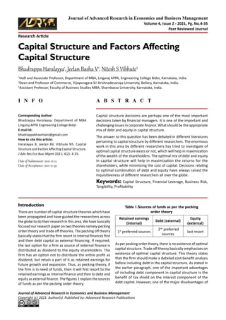
  • 1. Research Article Journal of Advanced Research in Economics and Business Management Copyright (c) 2021: Author(s). Published by: Advanced Research Publications Journal of Advanced Research in Economics and Business Management Volume 4, Issue 2 - 2021, Pg. No.4-35 Peer Reviewed Journal I N F O A B S T R A C T Corresponding Author: Bhadrappa Haralayya, Department of MBA Lingaraj APPA Engineering College Bidar. E-mail Id: bhadrappabhavimani@gmail.com How to cite this article: Haralayya B, Jeelan BV, Vibhute NS. Capital Structure and Factors Affecting Capital Structure. J Adv Res Eco Busi Mgmt 2021; 4(2): 4-35. Date of Submission: 2021-12-13 Date of Acceptance: 2021-12-30 Capital Structure and Factors Affecting Capital Structure Bhadrappa Haralayya1 , Jeelan Basha V2 , Nitesh S Vibhute­3 1 HoD and Associate Professor, Department of MBA, Lingaraj APPA, Engineering College Bidar, Karnataka, India. 2 Dean and Professor of Commerce, Vijayanagara Sri Krishnadevaraya University, Bellary, Karnataka, India. 3 Assistant Professor, Faculty of Business Studies MBA, Sharnbasva University, Karnataka, India. Capital structure decisions are perhaps one of the most important decisions taken by financial managers. It is one of the important and challenging issues in corporate finance. What should be the appropriate mix of debt and equity in capital structure. The answer to this question has been debated in different literatures pertaining to capital structure by different researchers. The enormous work in this area by different researchers has tried to investigate of optimal capital structure exists or not, which will help in maximization of the wealth of the shareholders. The optimal mix of debt and equity in capital structure will help in maximization the returns for the shareholders, while minimizing the cost of capital. Decisions relating to optimal combination of debt and equity have always raised the inquisitiveness of different researchers all over the globe. Keywords: Capital Structure, Financial Leverage, Business Risk, Tangibility, Profitability Introduction There are number of capital structure theories which have been propagated and have guided the researchers across the globe to do their research in this area. We have basically focused our research paper on two theories namely-pecking order theory and trade off theories. The pecking off theory basically states that the firm resort to internal finances first and then debt capital as external financing. If required, the last option for a firm as source of external finance is distributed as dividend to the equity shareholders. The firm has an option not to distribute the entire profit as dividend, but retain a part of it as retained earnings for future growth and expansion. Thus, as pecking theory, if the firm is in need of funds, then it will first resort to the retained earnings as internal finance and then to debt and equity as external finance. The figures 1 explain the sources of funds as per the pecking order theory. Retained earnings (internal) Debt (external) Equity (external) 1st preferred sources 2nd preferred sources last resort Table 1.Sources of funds as per the pecking order theory As per pecking order theory, there is no existence of optimal capital structure. Trade off theory basically emphasizes on existence of optimal capital structure. This theory states that the firm should make a detailed cost-benefit analysis before including debt in the capital structure. As stated in the earlier paragraph, one of the important advantages of including debt component in capital structure is the benefit of tax shield on the interest component of the debt capital. However, one of the major disadvantages of
  • 2. 5 Haralayya B et al. J. Adv. Res. Eco. Busi. Mgmt. 2021; 4(2) including debt in capital structure is that the financial risk increases because of the constant interest burden of the debt component. The finance manager should investigate the pros and cons of including debt component in the capital structure. Thus, an optimal capital structure can be achieved with an appropriate mixture of equity and debt in the capital structure so as to minimize the cost as well as maximize the returns. Our research paper has tried to investigate what deter- minants the capital structure of a firm during the recessionary period comprising of the pre and post period. It is very important to understand the determinants of capital structure before taking various crucial decisions related to capital structure in an organization. When we were scanning the different past literatures related to capital structure, it was observed that the determinants of capital structure different from one industry to the other. For example: the capital structure determinants for the textile industry differ from steel and cement industry. Thus we decided to take BSE30 for our research taking a cross section of different industries. It was prudent to take BSE30 for our research as the index represents 94% of the market capitalization of the BOMBAY STOCK EXCHANGE, which is a major and oldest stock exchange of INDIA. The index also covers all the 7 major industries of INDIA namely private and public banks, pharmaceutical, information technology, etc. Thus, we decided to take BSE30 for our study as it will include cross section industries of major sectors in INDIA rather than concentrating on one specific/ industries. Our entire research work has been segregated into pre- recession period and post -recession period. Pre-recession period has been taken from 2010-11 to 2014-2015 (total 5 years) and post-recession period is from 2015-16 to 2019- 2020 (total 5 years). Multiple regression analysis has been utilized in this study to understand the capital structure determinants for the firms which belong to BSE30 during the pre as well as post recession period. The dependent variable which has been taken in the study is “financial leverage “ and 10 independent variables have been taken as probable determinants of financial leverage or capital structure during the pre and post period of recession. Hence, the main purpose for conducting this study is to investigate the determinants of capital structure or financial leverage of BSE30 companies during the pre and post recession period. Objectives of the Study The major objective of the research study focused on the follows: To identify those independent variables which are significant determinants of capital structure (financial leverage) for the firms belonging to BSE30 during the pre and post recession period. To rank the above significant variables determining the financial leverage on the basis of their beta values. To further investigate whether the variables significantly determining the capital structure for BSE30 companies are reflected pecking order or trade off theory during the pre and post period of recession. Research Methodology Data Source The present study was taken into consideration the companies of BSE30. we derived a list of 30 companies belonging to the BSE for the year spanning from 2009 -2010 to 2019 - 2020,which is segregated as prerecession period from 2009-2010 to 2014-2015 and post recession period from 2015-2016 to 2019-2020. Overall, 30 companies, which satisfied all parameters, were utilized for the study. Statistical Methods Durbin Watson test has been used in this study to test if the data are having time series influence or not. If the data are stationary, then multiple recession analysis can be done, otherwise we have to go for panel recession. SPSS 20.0 software has been used to derive the correlation matrix between the financial leverage (which is taken as dependent variable) and the independent variables for both the pre and post recession period. With the help of this matrix, multi collinearity problem has been investigated. The correlation between the independent variable should be least for running multiple recession analysis. If the correlation among the independent variable is very high, then multicollinearity problem is assumed to exist and we cannot continue with the multiple recession analysis. High correlation has been defined in different researchers. Lewis-beck (1980) stated that if the correlation between the independent variables is equal to or more than. 80, then multicollinearity problems will be assumed to exist. This reference has been used in this research article. Thus, thought correlation matrix, multi- collinearity problem has been investigated and then multiple recessions have been applied taking one dependent variable (financial leverage) and 10 independent variables. Variables taken in the study Financial leverage is taken as a dependent variable in this research paper. Financial leverage is defined as average total assets divided by average total debt. Total debt includes the sum total of both borrowings and currently liability and provisions. It has been an endeavor in this study so as to understand the determinants of financial leverage by taking 10 independent variables. The table 1 consists of the details
  • 3. 6 Haralayya B et al. J. Adv. Res. Eco. Busi. Mgmt. 2021; 42) regarding the dependent and the independent variables taken for the study. The independent variable taken in the study may have some impact on financial leverage. Tangibility Tangibility has been defined in this research paper as average net fixed assets and average total assets. The trade off theory assumes a positive relation between tangibility and financial leverage. Profitability A return on assets has been taken as a proxy for profitability inthispaper.Oneoftheimportantparametersformeasuring the financial performance of a firm is by profitability. The tradeoff theory indicates a positive relationship between profitability and financial leverage. Pecking off theory, which prefers internal financing to debt component as source of finance, has profitability and financial leverage are negatively related to each other. Size of the firm Some of the major studies in the past have indicated a relation between size of the firm and financial leverage. Trade off basically states a positive relationship between size and financial leverage. A larger sized firm has better debt bearing capacity, but pecking order theory emphasized that size and financial leverage are negatively related to each other. Two proxies have been used for “size of the firm “in this research study, that is, log (total sales) and log (total assets). Interested coverage ratio: interest coverage ratio has been defined in this project as the ration between average earnings before interest and tax and average interest paid. Positive relation between interest coverage ratio and average financial leverage is supporting by the tradeoff theory, but on the other hand, the pecking order theory emphasizes that interest coverage ratio and financial leverage are negatively related to each other. Dividend Payout Ratio Dividend payout ratio is defined as the ratio between dividend and total income available to shareholders (profit after tax). Here, dividend includes only dividend paid and proposed. The tradeoff theory states that dividend payout ratio and financial leverage are positively related to each other. Non Debt tax shield Non debt tax shield has been defined in this article as the ratio between the deprecation and total assets. It is the tax deduction enjoyed by the business in the form of deprecation. Tradeoff theory confirms a negative relationship between financial leverage and non de bt tax shield. Degree of Operating Leverage Increase in degree of opera-ting leverage in turn increases thee fluctuation in the future profit earning. Operating leverage and debt level in capital structure are negatively related to each other. There is a greater chance that the business failure will increase if the degree of operating leverage increases. Hence, the organization will prefer lesser debt in the capital structure. Both the pecking order theory and tradeoff theory confirms a negatively relationship between degree of operating leverage and financial leverage. Growth rate Growthrateisanimportantdeterminantofcapitalstructure. Pecking order theory confirms a positive relationship between the growth rate (assets) and financial leverage. It states that the highly growth oriented firms will prefer more debt in their capital structure as their profitability will allow them a cushion against the cost of debt. Thus, if the growth opportunities are less, the organization will prefer lesser debt in the capital structure and it will rely more on internal financing. Trade off theory suggests a negative relationship between growth rate (assets) and financial leverage. If the growth opportunities increase, the firm will prefer less leverage and retained more profit in the business. Business risk One of the important variables in financial from dominant knowledge s business risk. It is defined as the co efficient of variables of earnings before interest and tax. With the increases of business risk, the volatility of the earning will also increase. Hence, the firm will prefer lesser debt in the capital structure because of increased business risk. Thus, the company will rely more internal financing rather than debt a as source of financing. A negative relation is expected between business risk and financial leverage. Third Module Concept of Capital Structure The capital structure of a company is made up of debt and equity securities that comprise a firm’s financing of its assets. It is the permanent financing of a firm represented by long-term debt, preferred stock and net worth. So it relates to the arrangement of capital and excludes short- term borrowings. It denotes some degree of permanency as it excludes short-term sources of financing The relative proportion of various sources of funds used in a business is termed as financial structure. Capital structure is a part of the financial structure and refers to the proportion of the various long-term sources of financing. It is concerned with making the array of the sources of the funds in a proper manner, which is in relative magnitude and proportion.
  • 4. 7 Haralayya B et al. J. Adv. Res. Eco. Busi. Mgmt. 2021; 4(2) Category Variable code Variable name Details Dependent FL Financial leverage Average total debt/average total assets Independent FL Interest coverage ratio Average PBIT/ average interest paid Profit- ability Return on assets Average PBIT/ average total assets BR Business risk Standard deviation of PBIT/average PBIT GR Growth rate (assets) Compound growth rate of total assets DOL Degree of operating leverage % change in PBIT to % change in sales Size_1 Size of the firm (1) Log (average total sales) Size_2 Size of the firm (2) Log(average total assets) TAN Tangibility Average net fixed assets/average total assets NDTS Non debt tax shield Average deprecation/ average total assets Meaning The term capital structure refers to the percentage of capital (money) at work in a business by type. Broadly speaking, there are two forms of capital: equity capital and debt capital. Each type of capital has its benefits and drawbacks and a substantial part of wise corporate stewardship and management is attempting to find the perfect capital structure regarding risk/reward payoff for shareholders. This is true for Fortune 500 companies as well as small business owners trying to determine how much of their start-up money should come from a bank loan without endangering the business. Equity Capital  Equity capital refers to money put up and owned by the shareholders (owners). Typically, equity capital consists of two types:  • Contributed capital: The money that was originally invested in the business in exchange for shares of stock or ownership • Retained earnings: Profits from past years that have been kept by the company and used to strengthen the balance sheet or fund growth, acquisitions, or expansion Many consider equity capital to be the most expensive type of capital a company can use because its “cost” is the return the firm must earn to attract investment. A speculative mining company that is looking for silver in a remote region of Africa may require a much higher return on equity to get investors to purchase the stock than a long-established firm such as Procter & Gamble, which sells everything from toothpaste and shampoo to detergent and beauty products. Debt Capital The debt capital in a company’s capital structure refers to borrowed money that is at work in the business. The cost depends on the health of the company’s balance sheet—a triple AAA rated firm can borrow at extremely low rates vs. a speculative company with tons of debt, which may have to pay 15% or more in exchange for debt capital. There are different varieties of debt capital: • Long-term bonds: Generally considered the safest type because the company has years, even decades, to come up with the principal while paying interest only in the meantime. • Short-term commercial paper: Used by giants such as Wal-Mart and General Electric, this amounts to billions of dollars in 24-hour loans from the capital markets to meet day-to-day working capital requirements such as payroll and utility bills. • Vendor financing: In this instance, a company can sell goods before they have to pay the bill to the vendor. This can drastically increase return on equity but costs the company nothing. One secret to Sam Walton’s success at Wal-Mart was selling Tide detergent before having to pay the bill to Procter & Gamble, in effect, using P&G’s money to grow his retail enterprise. Table 2.List of dependent and independent variables used in the study DPR Dividend payout ratio Average dividend/average PAT (Profit after Tax)
  • 5. 8 Haralayya B et al. J. Adv. Res. Eco. Busi. Mgmt. 2021; 42) • Policyholder“float”:Inthecaseofinsurancecompanies, this is money that doesn’t belong to the firm but that it gets to use and earn an investment on until it has to pay it out for auto accidents or medical bills. The cost of other forms of capital in the capital structure varies greatly on a case-by-case basis and often comes down to the talent and discipline of managers. Capital Structure A company’s capital structure points out how its assets are financed. When a company finances its operations by opening up or increasing capital to an investor (preferred shares, common shares, or retained earnings), it avoids debt risk, thus reducing the potential that it will go bankrupt. Moreover, the owner may choose debt funding and maintain control over the company, increasing returns on the operations. Debt takes the form of a corporate bond issue, long-term loan, or short-term debt. The latter directly impacts the working capital. Having said that, a company that is 70% debt-financed and 30% equity-financed has a debt-to-equity ratio of 70%; this is the leverage. It is very important for a company to manage its debt and equity financing because a favorable ratio will be attractive to potential investors in the business. From a technical perspective, the capital structure is defined as the careful balance between equity and debt that a business uses to finance its assets, day-to-day operations and future growth. From a tactical perspective however, it influences everything from the firm’s risk profile, how easy it is to get funding, how expensive that funding is, the return its investors and lenders expect and its degree of insulation from microeconomic business decisions and macroeconomic downturns. By design, the capital structure reflects all of the firm’s equity and debt obligations. It shows each type of obligation as a slice of the stack. This stack is ranked by increasing risk, increasing cost and decreasing priority in a liquidation event (e.g., bankruptcy). For large corporations, it typically consists of senior debt, subordinated debt, hybrid securities, preferred equity and common equity. Any company’s capital structure serves several key purposes. First and foremost, it’s effectively an overview of all the claims that different players have on the business. The debt owners hold these claims in the form of a lump sum of cash owed to them (i.e., the principal) and accompanying interest payments. The equity owners hold these claims in the form of access to a certain percentage of that firm’s future profit. Secondly, it is heavily analyzed when determining how risky it is to invest in a business and therefore, how expensive the financing should be. Specifically, capital providers look at the proportional weighting of different types of financing used to fund that company’s operations. For example, a higher percentage of debt in the capital structure means increased fixed obligations. More fixed obligations result in less operating buffer and greater risk. And greater risk means higher financing costs to compensate lenders for that risk (e.g., 14% interest rate vs 11% interest rate). Consequently, all else equal, getting additional funding for a business with a debt-heavy capital structure is more expensive than getting that same funding for a business with an equity-heavy capital structure. “Capital structure is essentially concerned with how the firm decides to divide its cash flows into two broad components, a fixed component that is earmarked to meet the obligations toward debt capital and a residual component that belongs to equity shareholders”-P. Chandra. Definition - What does Capital Structure mean? Capital structure refers to a company’s outstanding debt and equity. It allows a firm to understand what kind of funding the company uses to finance its overall activities and growth. In other words, it shows the proportions of senior debt, subordinated debt and equity (common or preferred) in the funding. The purpose of capital structure is to provide an overview of the level of the company’s risk. As a rule of thumb, the higher the proportion of debt financing a company has, the higher its exposure to risk will be. Capital structure is commonly known as the debt-to-equity ratio. Capital structure is the mix of the long term sources of funds used by the firm. It is made up of debt and equity securities and refers to permanent financing of a firm. It I composed of long term debt, preference share capital and shareholders fund. “Capital structure is essentially concerned with how the firm decides to divide its cash flows into two broad components, a fixed component that is earmarked to meet the obligations toward debt capital and a residual component that belongs to equity shareholders”-P. Chandra. “Capital structure of a company refers to the composition or make up of its capitalization and it includes all long term capital resources viz., loans, reserves, shares and bonds” Gerstenberg. Capital structure as, “balancing the array of funds sources in a proper manner, i.e. in relative magnitude or in proportions”- Keown et al. Hence capital structure implies the composition of funds raised from various sources broadly classified as debt and equity. It may be defined as the proportion of debt and
  • 6. 9 Haralayya B et al. J. Adv. Res. Eco. Busi. Mgmt. 2021; 4(2) equity in the total capital that will remain invested in a business over a long period of time. Capital structure is concerned with the quantitative aspect. A decision about the proportion among these types of securities refers to the capital structure decision of an enterprise. Importance of the Capital Structure Decisions relating to financial the assets of a firm are very crucial in every business and the financial managers is often caught in the dilemma of what the optimum proportion of debt and equity should be. As a general rule there should be a proper mix of debt and equity capital in financing the firm’s assets. Capital structure is usually designed to serve the interest of the equity shareholders. Description Value maximization: capital structure maximizes the market value of a firm, i.e in a firm having a properly designed capital structure the aggregate value of the claims and ownership interests of the shareholders are maximized. Cost minimization Capital structure minimizes the firm’s cost of capital or cost of financing. By determining a proper mix of funds sources, a firm can keep the overall cost of capital to the lowest. Increase in share price: capital structure maximizes the company’s market price of share by increasing earnings per share of the ordinary shareholders. It also increases dividend receipt of the shareholders. Investment opportunity Capital structure increases the ability of the company to find new wealth-creating investment opportunities. With proper capital gearing, it also increases the confidence of suppliers of debt. Growth of the country capital structure increases the country’s rate of investment and growth by increasing the firm’s opportunities to engage in future- creating investment. Increases in value of the firm A sound capital structure of a company helps to increases the market price of shares and securities which, in turn, lead to increase in the value of the firm. Utilization of available funds A good capital structure enables a business enterprise to utilize the available funds fully. Properly designed capital structures ensure the determinants’ of the financial requirements’ of the firm and raise the firm. Maximization of available funds A sound capital structure enables management you increase the profits of a company in the form of higher return to the equity shareholders i.e. increasing in earning per share. It can be done by mechanism of trading on equity. Minimization of cost of control A sound structure of any business enterprises maximizes shareholders’ wealth through minimization of the overall cost of capital. This can also be done by incorporation long-term debt capital in the capital structure as the cost of debt capitals lower than the cost of equity or preference share capital since the interest on debt is tax deductable. Solvency or liquidity position It never allows a business enterprise to go for too much rising of debt capital because, at the time of poor earning, the solvency is distributed for compulsory payment of interest to the debt-supplier. Flexibility A sound capital structure provides a room for expansion or reduction of debt so that, according to changing conditions, adjustment off capital can be made. Value maximization Cost minimization Cost minimization Investment opportunity Growth of the country Increase in value of the firm Utilization of available funds Maximization of cost of capital Solvency or liquidity position Flexibility Undistributed controlling Minimization of financial risk Undisturbed controlling It does not aloe the equity shareholder control on business to be diluted. Minimization of financial risk If debt component increase in the capital structure of a company, the financial risk also increases good financial capital structure helps in protecting the business enterprise from such financial risk through a judicious mix of debt and equity in the capital structure. Theory related to capital structure Pecking order theory History Pecking order theory was first suggested by Donaldson in 1961 and it was modified by Stewart C. Myers and Nicolas Majluf in 1984. It states that companies prioritize their sources of financing (from internal financing to equity) according to the cost of financing, preferring to raise equity Table 3
  • 7. 10 Haralayya B et al. J. Adv. Res. Eco. Busi. Mgmt. 2021; 42) as a financing means of last resort. Hence, internal funds are used first and when that is depleted, debt is issued and when it is not sensible to issue any more debt, equity is issued. Theory Pecking order theory starts with asymmetric information as managersknowmoreabouttheircompany’sprospects,risks and value than outside investors. Asymmetric information affects the choice between internal and external financing and between the issue of debt or equity. Therefore, there exists a pecking order for the financing of new projects. Asymmetric information favours the issue of debt over equity as the issue of debt signals the board’s confidence that an investment is profitable and that the current stock price is undervalued (were stock price over-valued, the issue of equity would be favoured). The issue of equity would signal a lack of confidence in the board and that they feel the share price is over-valued. An issue of equity would therefore lead to a drop in share price. This does not however apply to high-tech industries where the issue of equity is preferable due to the high cost of debt issue as assets are intangible. Trade off theory The trade-off theory of capital structure is the idea that a company chooses how much debt finance and how much equity finance to use by balancing the costs and benefits. The classical version of the hypothesis goes back to Kraus and Litzenberger who considered a balance between the dead-weight costs of bankruptcy and the tax saving benefits of debt. Often agency costs are also included in the balance. This theory is often set up as a competitor theory to the pecking order theory of capital structure. A review of the literature is provided by Frank and Goyal. An important purpose of the theory is to explain the fact that corporations usually are financed partly with debt and partly with equity. It states that there is an advantage to financing with debt, the tax benefits of debt and there is a cost of financing with debt, the costs of financial distress includingbankruptcycostsofdebtandnon-bankruptcycosts (e.g. staff leaving, suppliers demanding disadvantageous payment terms, bondholder/stockholder infighting, etc.). The marginal benefit of further increases in debt declines as debt increases, while the marginal cost increases, so that a firm that is optimizing its overall value will focus on this trade-off when choosing how much debt and equity to use for financing. Agency theory The principal-agent problem, in political science and economics (also known as agency dilemma or the agency problem) occurs when one person or entity (the “agent”), is able to make decisions and/or take actions on behalf of, or that impact, another person or entity: the “principal”. This dilemma exists in circumstances where agents are motivated to act in their own best interests, which are contrary to those of their principals and is an example of moral hazard. Common examples of this relationship include corporate management (agent) and shareholders (principal), elected officials (agent) and citizens (principal), or brokers (agent) and markets (buyers and sellers, principals). Consider a legal client (the principal) wondering whether their lawyer (the agent) is recommending protracted legal proceedings because it is truly necessary for the client’s well being, or because it will generate income for the lawyer. In fact the problem can arise in almost any context where one party is being paid by another to do something where the agent has a small or nonexistent share in the outcome, whether in formal employment or a negotiated deal such as paying for household jobs or car repairs. The problem arises where the two parties have different interests and asymmetric information (the agent having more information), such that the principal cannot directly ensurethattheagentisalwaysactingintheir(theprincipal’s) best interest,particularly when activities that are useful to the principal are costly to the agent and where elements of what the agent does are costly for the principal to observe (see moral hazard and conflict of interest). Often, the principal may be sufficiently concerned at the possibility of being exploited by the agent that they choose not to enter into the transaction at all, when it would have been mutually beneficial: a suboptimal outcome that can lower welfare overall. The deviation from the principal’s interest by the agent is called “agency costs”. The agency problem can be intensified when an agent acts on behalf of multiple principals (see multiple principal problem). When one agent acts on behalf of multiple principals, the multiple principals have to agree on the agent’s objectives, but face a collective action problem in governance, as individual principals may lobby the agent or otherwise act in their individual interests rather than in the collective interest of all principals.As a result, there may be free-riding in steering and monitoring, duplicate steering and monitoring, or conflict between principals, all leading to high autonomy for the agent. This has been coined the multiple principal problem and is a serious problem in particularly the public sector, where multiple principals are common and both efficiency and democratic accountability are undermined in the absence of salient governanceVarious mechanisms may be used to align the interests of the agent with those of the principal. In employment, employers (principal) may use piece rates/ commissions, profit sharing, efficiency wages, performance measurement (including financial statements), the agent posting a bond, or the threat of termination of employment to align worker interests with their own.
  • 8. 11 Haralayya B et al. J. Adv. Res. Eco. Busi. Mgmt. 2021; 4(2) Table 4.Pre- results (2009-2010:2013-2014) BR DOL DP FL GR ICR NDTS ROA SF1 SF2 TAN Mean 0.4772 0.8394 0.3279 0.2585 14.8357 120.6225 0.0228 0.1492 9.8455 10.7620 0.2661 Median 0.2437 0.8285 0.2773 0.1281 14.4947 10.37152 0.0207 0.1199 10.2640 10.5346 0.2323 Maximum 4.6148 5.6894 0.9228 0.8766 26.9862 932.7109 0.0806 0.3692 12.6252 14.1479 0.8504 Minimum 0.0805 -2.0020 0.0433 0.0000 -0.6961 -8.7540 0.0002 0.0078 5.9610 8.4897 0.0043 Std. Dev. 0.8230 1.1379 0.2159 0.3037 6.9594 246.8580 0.0202 0.1168 1.3839 1.4346 0.2147 Skewness 4.4780 2.1186 1.0929 11259 -0.3769 2.1558 1.3326 0.4748 -0.8667 0.4053 0.7312 Kurtosis 22.8615 13.2576 3.6011 2.7194 2.7008 6.3079 4.5610 1.8907 3.9361 2.3911 3.0864 Jarque-Bera 593.3606 153.9654 6.4235 6.4365 0.8220 36.9157 11.9244 2.6652 4.8511 1.2846 2.6825 Probability 0.0000 0.0000 0.0403 0.0400 0.6630 0.0000 0.0026 0.2638 4.8511 0.5261 0.2615 Sum 14.3172 25.1819 9.8358 7.7553 445.0707 3618.6740 0.6832 4.4753 295.3659 322.8602 7.9827 Sum Sq. Dev. 19.6408 37.5491 1.3520 2.6752 1404.5519 1767228.0000 0.0118 0.3958 55.5430 59.6810 1.3363 Observations 30 30 30 30 30 30 30 30 30 30 30 Coefficient of variables 1.7244 1.7244 0.6586 0.6586 0.46691 2.0465 0.8850 0.7831 0.1406 59.6810 1.3363
  • 9. 12 Haralayya B et al. J. Adv. Res. Eco. Busi. Mgmt. 2021; 42) Table 5.Pre-Correlation Matrix BR DOL DP FL GR ICR NDTS ROA SF1 SF1 TAN BR 1.0000 -0.4476 0.1430 -0.0771 0.1158 -0.0519 0.1146 -0.2081 -0.3583 -0.2278 -0.1446 DOL -0.4476 1.0000 0.4159 -0.2981 -0.2946 0.1141 -0.0648 0.5326 -0.3614 -0.1813 -0.0109 DP 0.1430 0.4159 1.0000 -0.2981 -0.5383 0.3517 0.0092 0.5404 -0.2142 -0.2641 -0.0699 FL -0.0771 -0.2981 -0.3640 1.0000 0.2753 -0.3770 -0.4867 -0.7497 0.0928 0.7411 -0.3175 GR 0.1158 -0.2946 -0.5383 0.2753 1.0000 -0.2139 -0.2681 0.1392 -0.1868 -0.0405 -0.0519 ICR -0.1441 0.1141 0.3517 -0.3770 -0.2139 1.0000 0.3373 0.5620 0.1726 -0.1578 0.1146 NDTS -0.1893 -0.0648 0.0092 -0.4867 -0.2681 0.3373 1.0000 0.2296 0.2625 -0.2844 0.6059 ROA -0.2081 0.5326 0.5404 -0.7497 -0.1392 0.5620 0.2296 1.0000 -0.1421 -0.6261 0.0124 SF1 -0.3583 -0.3614 -0.2142 0.0928 0.1868 0.1726 0.2625 -0.1421 1.0000 0.5473 0.1630 SF1 -0.2278 -0.1813 -0.2142 0.7411 -0.0405 -0.1578 0.2625 -0.6261 1.0000 1.0000 0.1630 TAN 0.1446 -0.0109 -0.0699 -0.3175 -0.0519 0.1146 0.6059 -0.6261 0.1630 -0.1455 1.0000 Fourth module Interpretation and analysis The given above Table 4 includes the results of the given independent variables and dependent variable of capital structures. The following are the indication and explanation on the Table 4. 1. Mean: It implies the average and it is sum of set of data divided by the number of data. MEAN can is an effective tool when compared to different sets of data. The highest value from the variables are ICR=120.6225, GR=14.8357 and the lowest value are ROA=.1492, FL=.2585. 2. Median: It is the middle value when the data is arranged in numerical order. It is another effective tool to compare different sets of data. The negative impact of extreme values is lesser on median compared to mean. The highest variables with the value are GR=14.4947, SF (2) =10.5346 and the lowest value are ROA=0.1199, FL=0.1281. 3. Maximum: The highest value based variables are ICR=932.7109, GR=26.9862 and the lowest value based variables are NDTS=0.0806, ROA=0.3692. 4. Minimum: The highest value from the above variables are SF (2) =8.4897, SF (1) =5.9610 and the lowest value based variables are ICR=-8.7540, DOL=-2.0020. 5. Standard deviation: It is the measure of the average distance between the values of the data in the set and the mean. The higher standard deviation from the variables are ICR=246.8580, GR=6.9594 and the lowest standard deviation are NDTS=0.0202, ROA=0.1168 6. Skewness: It measures whether the data are heavy lopsidedness or lightly lopsidedness relative to a normal distribution. It indicates the shape of the distributed data .the highest variables are BR=4.4780, ICR=2.1558 and the lowest are SF (1) =-0.8667, GR=-0.3769. 7. Kurtosis: It is used to measure whether the data are heavy-tailed or light tailed relative to a normal distribution. It measures the data peak and flatness of the normal distribution. The highest value are BR=22.8615, DOL=13.2576 and the lowest are NDTS=1.8907, SF (2) =2.3911. 8. Jarque-bera test: This test is a goodness of fit test of whether sample data have the skewness and kurtosis matching the normal distribution. The highest vales from the variables are BR=593.3606, DOL=153.9654 and the lowest values are GR=0.8220, SF (1) =1.2846. 9. Probability: The values of the variable are based on the underlying probability distribution. The highest probability variables are SF (1) =0.5261, ROA=0.2638 and lowest are BR=0.000, DOL=0000. 10. Sum: The total value of the variables influenced with the higher value are ICR=3618.6740, GR=445.0707 and lowest value are NDTS=.6832, ROA=4.4753. 11. Sum of square deviation: the highest value are ICR=1767228.0000, GR=1404.5510 and lowest value are NDTS=0.0118, ROA=0.3958. 12. Observation: The total variables in the given table.
  • 10. 13 Haralayya B et al. J. Adv. Res. Eco. Busi. Mgmt. 2021; 4(2) no-1 all the variables total observations are 30 taken into consideration. 13. Co-efficient of variables: It is the ratio between the standard deviation to the mean. The highest variable are ICR=2.0465, BR=1.7244 and the lowest variables are SF (1)0.1406, SF (2) =0.1333. The following data represented in the table. No 4 are the pre-results of the dependent and independent variable that affects the capital structure of the companies. A correlation matrix is a table showing co-efficient between the variables taken in the data analysis. A correlation matrix is used to summarize data to make key decisions including choice of correlation statistic, coding of the variables and treatment of missing data and presentation. Typically a correlation matrix is “square” with the same variables shown in the rows and columns. This shows the correlation between the different variables. The given table no. 5 the correlation matrix helps to identify the relationship between the different variables with each other variable along with the given data. given data. It helps and allows you to determine which factors matter most and factor can be ignored. In order to understand the regression analysis it is necessary to understand the following terms: dependent variables and independent variables. Dependent variables: the main factor that we are trying to understand or predict. (I.e. financial leverage). Independent variables: the factors that are hypothesized and have an impact on the dependent variable.(I.e. ICR, ROA, BR, GR, DOL, SF(1), SF(2), TANG, NDTS, DPR.). In the given table 6, only the variables that are influenced by the dependent variables with that of independent variable are included with data as per there analyzed values of the calculated regression values. In the given table 6, the dependent variables that are influenced and accepted with given regression test condition’s of the data which includes the variables that are ROA, BR, GR, DOL, SF(1), SF(2), TAN and DPR. These are the variables that are accepted with given conditions along with the given data. These factors are further utilized for the statistical method and data analyzed with following tests which includes r-square value 0.906501, adjusted R-squared calculated value 0.870882, P-value values 3.86e-09x (negative value) and Durbin Watson test value 1.722701. Where these test are proved and accepted with data analyses and results thereof. The given Table 7, includes the results of different tests done to prove the given statistical data. It includes no of test done, name of the tests, null hypothesis (Ho), p-value or results of the test and acceptance or rejection of the null hypothesis after the examination of the data. The given null hypothesis of the specified tests are accepted only when the given results or p-value is more than or equal to 0.05 (p-value>=0.05) and the null hypothesis is rejects when the given p-value or results are less than 0.05(p-value<0.05). these are the conditions of acceptance and rejection of the given test between the dependent and independent variables. The following are the name of the tests and their decision of acceptance and rejection based on the hull hypothesis criteria. Reset Test: This is the general specification test for finding the relationship of the independent and dependent variables. The given null hypothesis states that “specification is adequate”. The result of the given data is 5.03e-05(negative value). As the results is less than the criteria (I, e.5.03e-05<0.05). Hence the null hypothesis is rejected. Breuch Pagan test for Heteroscedasticity: The null hypothesis of the test statistic has a p-value below the appropriate threshold. The given null hypothesis states “heteroskrdasticity is not present” between the variables. Coefficient Std. Error t-ratio p-value Const 0.0543 0.3059 0.1776 0.8607 ROA -1.21755 0.4839 -2.516 0.0201 BR -0.169220 0.0401 -4.223 0.0004 GR 1.0172 0.4658 2.1840 0.0405 DOL -0.0956939 0.0407 -2.353 0.0284 SF1 -0.0989235 0.0361 -2.740 0.0123 SF2 0.1224 0.0360 3.3960 0.0027 TAN -0.273430 0.1096 -2.495 0.0210 DPR 0.3824 0.1753 2.1820 0.0406 Table 6.Pre-Regression table R-squared 0.906501 Adjusted R-squared 0.870882 P-value(F) 3.86e-09x Durbin-Watson 1.722701 In the given Table 5, the given matrix is the result of different variables multiplied with each and every factor variables which affects the companies and their capital structure. The line of 1.0000 from left top of the matrix till the right bottom of the matrix a cross line slopes downwards with the same results of 1.0000. This indicates that in the given matrix (Table 5) the variables which are calculated with it are more relative than any other variables in the given data. Regression analysis is the powerful statistical method that allows you to determine the relationship between two or more variables. The examination of one or more independent variables and dependent variables on the
  • 11. 14 Haralayya B et al. J. Adv. Res. Eco. Busi. Mgmt. 2021; 42) The results of the test is 0.66398 which is more than the accepted criteria (i.e. 0.66398>=0.05). Hence the given null hypothesis is accepted. Normality of Residual: If the data set is well modeled by a normal distribution. The null hypothesis of normality states that “error is normally distributed”. The given results of the test statics is 0.257238 which is more than the stated criteria (i.e. 0.257238>=0.05). Hence the null hypothesis is accepted. Chowtest for structural Distribution: As the given data is on the basis of pre and post calculation here the term is assumed to be the same in both periods. The null hypothesis states that “no structural break”. The results of the test is 0.884201 greater then 0.05 (i.e. 0.884201>=0.05). Hence the null hypothesis is accepted. LM for auto Correlation up to order 1: The null hypothesis of the given data states that “no autocorrelation”. The results of the given data is 0.534286 greater than 0.05 (i.e. 0.534286>=0.05). Hence the null hypothesis is accepted. ARCH of Order 1: The null hypothesis of the test states that” no ARCH effect is present between the dependent and independent variables. The results of the given data and test is 0.543447 which is more than the 0.05 criteria (i.e. 0.543447>=0.05). Hence the null hypothesis is accepted. QLR test for Structural break: The null hypothesis of the given data states “no structural break”. The results of the given test is 0.142243 which is greater than the 0.05 criteria (I.e. 0.142243>=0.05). Hence the null hypothesis is accepted. Cusum Test for Parameter Stability: The null hypothesis of the given data states” no change in parameters”. The result of the given data is 0.0918764 which is greater than the 0.05 (i.e. 0.0918764). The null hypothesis is accepted. Variance Influencing Factors (VIF): VIF detects VIF (j) = 1/ (1 - R (j) ^2), where R (j) is the multiple correlation coefficient. Between variable j and the other independent variables. Variance inflation factors ranged from 1 upwards. The numerical value for VIF tells you what percentage of the variance is inflated for each co-efficient. In the given table we can justify that all the dependent variables are calculated with each other and every factor of the variables. From the table no 8, specifies clearly that the given variables are correlated with the given VIF tests under which the variables that results are between 5-10 are highly correlated. The results are given after the examination and calculation of the data under which the variables that highly correlated are ROA=7.782, DOL=5.212, SF (1) =6.077 and SF (2) =6.511. these variables are more relative and acceptable value of the variables. S. No. Test HO P-value/ Result Acceptance/ Rejection 1. Rest test Specification is adequate 5.13E-05 Rejected 2. Breusch-pagan test for heteroskedasticity Heteroskedasticity not nresent 0.66398 Accepted 3. normality of residuals Error is normally distributed 0.257238 Accepted 4. chow test for structural Break at obsevation no structural break 0.884201 Accepted 5. LM test for autocorrelation upto order-1 No autocorrelation 0.534286 Accepted 6. ARCH of order-1 No ARCH effect is present 0.543447 Accepted 7. QLR test for structrual break No structural break 0.142242 Accepted 8. CUSUM test for parmeter stability No change in parameters 0.0918764 Accepted Table 7.Pre- test analysis multicollinearity in regression analysis. Multicollinearity is when there’s correlation between independent variables in a model. Independent factors p-value Correlates results ROA 7.782 Correlates results BR 2648 Highly correlated GR 2.559 Moderated correalted DOL 5.212 Highly correalted SF1 6.077 Highly correalted SF2 6.511 Highly correalted TAN 1.348 Moderated correalted DPR 7.782 3.486 Moderated correalted Table 8.Pre variance influencing factors
  • 12. 15 Haralayya B et al. J. Adv. Res. Eco. Busi. Mgmt. 2021; 4(2) Table 9.Post Descriptive Post Descriptive Table BR DOL DP FL GR ICR NDTS ROA SF1 SF2 TAN Mean 0.2267 0.8154 0.2601 0.2692 11.4477 128.0691 0.0224 0.1423 10.3133 11.3845 0.2618 Median 0.1956 0.9979 0.2750 0.1233 12.0887 4.2773 0.0191 0.0887 10.7088 11.1079 0.2490 Maximum 4.4687 1.4257 0.9496 0.8881 30.9965 1863.7790 0.0618 0.6486 12.5882 14.8569 0.8491 Minimum -2.8960 -0.3718 -1.7475 0.0000 -3.7109 -253.1280 0.0008 -0.0165 5.7089 9.2249 0.0040 Std. Dev. 1.1439 0.5045 0.4380 0.3203 6.9492 368.0821 0.0175 0.1555 1.4029 1.4666 0.2277 Skewness 0.6263 -1.3160 -3.1356 0.9201 0.1520 3.7424 0.5369 1.4596 -1.3945 0.4611 0.8608 Kurtosis 10.0806 3.6277 16.0957 2.3060 3.8916 17.8430 2.4518 5.0095 5.5155 2.3704 3.0461 Jarque-Bera 64.6300 9.1520 263.5314 4.8353 1.1093 345.4200 1.8167 15.6996 17.6325 1.5586 3.7076 Probability 0.0000 0.0103 0.0000 0.0891 0.5743 0.0000 0.4032 0.0004 0.0001 0.4587 0.1566 Sum 6.7998 24.4626 7.8024 8.0763 343.4301 3842.0720 0.6729 4.2685 309.4000 341.5334 7.8532 Sum Sq. Dev. 37.9447 7.3807 5.5633 2.9758 1400.4400 3929049.0000 0.0089 0.7009 57.0786 62.3777 1.5040 Observations 30 30 30 30 30 30 30 30 30 30 30 Coefficient of variation 5.0467 0.6187 1.6841 1.1899 0.6070 2.8741 0.7806 1.0927 0.1360 0.1288 0.8700
  • 13. 16 Haralayya B et al. J. Adv. Res. Eco. Busi. Mgmt. 2021; 42) Table 10.Post Correlation matrix BR DOL DP FL GR ICR NDTS ROA SF1 SF2 TAN BR 1.0000 -0.4476 0.1430 -0.0771 0.1158 -0.1441 -0.1893 -0.2081 -0.3583 -0.2278 -0.1446 DOL -0.4476 1.0000 0.4159 -0.2981 -0.2946 0.1141 -0.0648 0.5326 -0.3614 -0.1813 -0.0109 DP 0.1430 0.4159 1.0000 -0.3640 -0.5383 0.3517 0.0092 0.5404 -0.2142 -0.2641 -0.0699 FL -0.0771 -0.2981 -0.3640 1.0000 0.2753 -0.3770 -0.4867 -0.7497 0.0928 0.7411 -0.3175 GR 0.1158 -0.2946 -0.5383 0.2753 1.0000 -0.2139 -0.2681 -0.1392 -0.1868 -0.0405 -0.0519 ICR -0.1441 0.1141 0.3517 -0.3770 -0.2139 1.0000 0.3373 0.5620 0.1726 -0.1578 0.1146 NDTS -0.1893 -0.0648 0.0092 -0.4867 -0.2681 0.3373 1.0000 0.2296 0.2625 -0.2844 0.6059 ROA -0.2081 0.5326 0.5404 -0.7497 -0.1392 0.5620 0.2296 1.0000 -0.1421 -0.6261 0.0124 SF1 -0.3583 -0.3614 -0.2142 0.0928 -0.1868 0.1726 0.2625 -0.1421 1.0000 0.5473 0.1630 SF2 -0.2278 -0.1813 -0.2641 0.7411 -0.0405 -0.1578 -0.2844 -0.6261 0.5473 1.0000 -0.1455 TAN -0.1446 -0.0109 -0.0699 -0.3175 -0.0519 0.1146 0.6059 0.0124 0.1630 -0.1455 1.0000 The table 8, consists of the post calculation of the descriptive valuesandvariablesdeterminingtheirbasicdataanalysisare done in order to determine the relationship and difference between the dependent and independent variable. 1. MEAN: It is the efficient tool used to determine the values and relationship of the variables between each other. In the table.no-5 the highest carried mean for the variables are ICR=128.0691, GR=11.4477 and the lowest variable values are NDTS=0.0224, ROA=0.1423. 2. Median: It is the tool used to find out the middle values of the variables or statistical data given and provided. It also referred as another tool to compare the different sets of data. The highest value of the variable are GR=12.0887, SF (1)= 11.7088 and the lowest variable are NDTS=0.0191, BR= 0.01956. 3. Maximum: The highest values of the variable from the given data are ICR= 1863.7790, GR= 30.9965 and the lowest values of the variable are NDTS= 0.0618, ROA=0.6486. 4. Minimum: The highest values of the variable from the given data are SF (1)= 9.2249, SF (2)= 507089 and the lowest values in the data are GR= -3.7109, BR= -2.8960. 5. Standard deviation: A higher standard deviation indicated that the given data points are spread out over a large range of values. The highest value are ICR=368.0821, GR=6.9492 and lowest values of the variable are NDTS=0.0175, DP=0.4380. 6. Skewness: It measure of the data that are heavy lopsidedness and light lopsidedness related to a normal distribution. It is a curve that indicates the data are analyzed and assured. The longest slop cure are ICR=3.7424, GR=1.4596 and the lowest variables with lowest curve are ICR= -3.1356, DOL= -1.3160. 7. Kurtosis: It measures whether the data are heavy tailed or light tailed relative to a normal distribution. It ensures and finds out the flatness and peakness of the data. The highest peakness of the values of the variables are ICR=17.8430, DP=16.0957 and the flatness of the data are FL=2.3060, SF (2)= 2.3704. 8. Jarque-bera: It is the test that indicates the goodness of fit test of whether the sample data are matching with the skewness and kurtosis of normal distribution. The highest match of the samples are ICR=345.4200, DR=263.5314 and the lowest match of the samples are GR=1.1093, SF (2)= 1.5586. 9. Probability: It is the function that describes the possible values that random variables can assume. The highest probability of the variables are GR=0.5743, SF (2) =0.4587 and the lowest probability of the variables are BR=0.0000, DP= 0.0000. 10. Sum: The total of all the variables values that are calculated to know the overall results of the sample. In the given data base the highest value of the variables are ICR=3842.0720, GR=343.4301 and the lowest values are NDTS=0.6729, ROA= 4.2685. 11. Sum square of deviation: The highest values of the variables are ICR=3929049.000, GR=1400.4400 and the lowest values of the variable are NDTS=0.0089, ROA=0.7009. 12. Observation: The overall observations taken for the data interpretation are of 30 companies that is used for analyzing the data and results. The overall observations are 30. 13. Co-efficient of variables: It is the ratio between the standard deviation and mean. The highest value of the variables are BR=5.0467, ICR=2.8741 and the lowest values of the variable are SF (2) =0.1288, SF (1) =0.1360.
  • 14. 17 Haralayya B et al. J. Adv. Res. Eco. Busi. Mgmt. 2021; 4(2) S. No. Tests HO p-value- results Acceptance/ Rejection 1. RESET test Specification is adequate 0.0002 Rejection 2. Breusch-pagan test for heteroskedasticity Heteroskedasticity not nresent 0.9162 Acceptance 3. Normality of residuals Error is normally distributed -3.635 Acceptance 4. Chow test for structural break at obsevation no structural break 0.8976 Rejection 5. LM test for Sutocorrelation upto order-1 No autocorrelation 0.0762 Acceptance 6. ARCH of order-1 No ARCH effect is present 0.1803 Acceptance 7. QLR test for structrual break No structural break 0.1273 Acceptance 8. CUSUM test for parmeter stability No change in parameters 0.3434 Acceptance Table 12.Post Test Analysis A correlation matrix is a table showing co-efficient between the variables taken in the data analysis. A correlation matrix is used to summarize data to make key decisions including choice of correlation statistic, coding of the variables and treatment of missing data and presentation. Typically a correlation matrix is “square” with the same variables shown in the rows and columns. This shows the correlation between the different variables. In the given table.no-7 the correlation matrix helps to identify the relationship between the different variables with each other variable along with the given data. In the given table 9, the given matrix is the result of different variables multiplied with each and every factor variables which affects the companies and their capital structure post years correlation matrix. The line of 1.0000 from left top of the matrix till the right bottom of the matrix a cross line slopes downwards with the same results of 1.0000. This indicates that in the given matrix ( table 9) the variables which are calculated with it are more relative than any other variables in the given data. Table no. 10 Regression analysis is the powerful statistical method that allows you to determine the relationship between two or more variables. The examination of one or more independent variables and dependent variables on the given data .it helps and allows you to determine which factors matter most and factor can be ignored. In order to understand the regression analysis it is necessary to understand the following terms: dependent variables and independent variables. Dependent variables: the main factor that we are trying to understand or predict. (I.e. financial leverage). Table 11.Post- correlation matrix R-squared 0.8828 Adjusted R-squared 0.8381 P-value(F) 3.85E-08 Durbin-Watson 1.6530 Coefficient Std. Error t-ratio p-value Const 0.0257122 0.371932 0.06913 0.9455 ROA -1.07546 0.371932 -3.635 0.0015 BR -0.0356657 0.0307231 -3.635 0.2587 GR 0.00747675 0.0044414 -3.635 0.1071 DOL -0.120352 0.0635683 -1.893 0.0722 SF1 -0.0815202 0.0235636 1.893 0.0023 SF2 -0.0815202 0.0330919 3.456 0.0024 NOTS -4.75587 1.96806 -2.417 0.0249 OP 0.240059 0.101271 2.37 0.027
  • 15. 18 Haralayya B et al. J. Adv. Res. Eco. Busi. Mgmt. 2021; 42) Independent variables: the factors that are hypothesized and have an impact on the dependent variable.(I.e. ICR, ROA, BR, GR, DOL, SF(1), SF(2), TANG, NDTS, DPR.) In the given table 10 only the variables that are influenced by the dependent variables with that of independent variable are included with data as per there analyzed values of the calculated regression values. In the given table no 11 the dependent variables that are influenced and accepted with given regression test condition’s of the data which includes the variables that are ROA, BR, GR, DOL, SF(1), SF(2), TAN and DPR. These are the variables that are accepted with given conditions along with the given data in post regression. These factors are further utilized for the statistical method and data analyzed with following tests which includes r-square value 0.8828, adjusted R- squared calculated value 0.8381, P-value values 3.85e-08(negative value) and Durbin Watson test value 1.6530. Where these test are proved and accepted with data analyses and results thereof. The above given table no. 11 includes the results of different tests done to prove the given statistical data of post period. It includes no of test done, name of the tests, null hypothesis (Ho), p-value or results of the test and acceptance or rejection of the null hypothesis after the examination of the data. The given null hypothesis of the specified tests are accepted only when the given results or p-value is more than or equal to 0.05 (p-value>=0.05) and the null hypothesis is rejects when the given p-value or results are less than 0.05(p-value<0.05).these are the conditions of acceptance and rejection of the given test between the dependent and independent variables. The following are the name of the tests and their decision of acceptance and rejection based on the hull hypothesis criteria. Rest Test: This is the general specification test for finding the relationship of the independent and dependent variables. The given null hypothesis states that “specification is adequate”. The result of the given data is 0.0002. As the results is less than the criteria (i, e.0.0002<0.05). Hence the null hypothesis is rejected. Breuch Pagan test for Heteroskrdasticity: the null hypothesis of the test statistic has a p-value below the appropriate threshold. The given null hypothesis states “heteroskrdasticity is not present” between the variables. The results of the test is 0.9162 which is more than the accepted criteria (i.e. 0.9162>=0.05). Hence the given null hypothesis is accepted. Normality of Residual: if the data set is well modeled by a normal distribution. The null hypothesis of normality states that “error is normally distributed”. The given results of the test statics is 0.8976 which is more than the stated criteria (i.e. 0.8976>=0.05). hence the null hypothesis is accepted. CHOWTEST for structural distribution: as the given data is on the basis of pre and post calculation here the term is assumed to be the same in both periods. The null hypothesis states that ‘no structural break”. The results of the test is 0.0486 lesser then 0.05(i.e. 0.0486<=0.05). Hence the null hypothesis is rejected. LM for auto correlation up to order 1: The null hypothesis of the given data states that “no autocorrelation”. The results of the given data is 0.7962 greater than 0.05 (i.e. 0.7962>=0.05). Hence the null hypothesis is accepted. ARCH of order 1: The null hypothesis of the test states that” no ARCH effect is present between the dependent and independent variables. The results of the given data and test is 0.1803 which is more than the 0.05 criteria (i.e. 0.1803>=0.05). Hence the null hypothesis is accepted. QLR test for structural break: the null hypothesis of the given data states “no structural break”. The results of the given test is 0.1273 which is greater than the 0.05 criteria (I.e. 0.1273>=0.05). Hence the null hypothesis is accepted. Cusum Test for Parameter Stability: the null hypothesis of the given data states” no change in parameters”. The result of the given data is 0.3434 which is greater than the 0.05 (i.e. 0.3434>=0.05). The null hypothesis is accepted. Variance influencing factors (VIF): VIF detects multi collinearity in regression analysis. Multicollinearity is when there’s correlation between independent variables in a model. Pre- variance Influencing factors Independent factors p-value Correlates results ROA 7.782 Highly correlated BR 2.648 Moderated correalted GR 2.559 Moderated correalted DOL 5.212 Highly correlated SF1 6.077 Highly correlated SF2 6.511 Highly correlated TAN 1.348 Moderated correalted DPR 3.486 Moderated correalted Table 13.Pre Variance influencing factors VIF (j) = 1/ (1 - R (j) ^2), where R (j) is the multiple correlation coefficient. Between variable j and the other independent variables. Variance inflation factors ranged from 1 upwards. The numerical value for VIF tells you what percentage of the variance is inflated for each co-efficient.
  • 16. 19 Haralayya B et al. J. Adv. Res. Eco. Busi. Mgmt. 2021; 4(2) In the given table we can justify that all the dependent variables are calculated with each other and every factor of the variables of the post data analysis. From the table 13 specifies clearly that the given variables are correlated with the given VIF tests under which the variables that results are between 5-10 are highly correlated. The results are given after the examination and calculation of the data under which the variables that moderately correlated. But no results of the given table 13 are highly correlated under the test. The variables that moderately correlated with the results are ROA = 3.695, BR = 2.157, GR = 1.664, DOL = 1.909, SF(1) = 1.909, SF(2) = 4.114, NDTS = 2.073 and DP = 3.436. These statically data are moderately correlated but not highly correlated between 5-10. Fifth Module Finding and Solutions 1. Pre -descriptive analysis indicates the relationship of independent variables with the basic calculations where the value of mean = ICR, median = GR, maximum = ICR, minimum = SF (2), standard deviation = ICR, skewness=BR,kurtosis=BR,jarue-bera=BR,probability = SF (1), sum = ICR, sum square deviation = ICR and coefficient of variables = ICR. 2. Pre-correlationmatrixexplainsthecorrelationbetween independent variables with each other independent variables. 3. Pre-regression analysis allows determining the relationship between 2 or more variables. The GR is highly correlated .where R-square 0.906501, adjusted R-square = 0.870882, P-value (f) = 3.86e-09x and Durbin Watson = 1.722701. 4. Pre-test analysis where statistical test under null hypothesis are accepted and rejected based on the accepted value 0.05.where RESET TEST is rejected and other test are accepted. 5. Pre-Variance influencing factor justify that all the dependent variables are calculated with each and every factor of the variable. Under these variables are highly correlated to ROA, DOL, SF (1) and SF (2). Where other variables are rejected. 6. Post-descriptive analysis where the value highest values of variables. Where mean = ICR, median = GR, maximum = ICR, minimum = SF (1), standard deviation = ICR, skewness = ICR, kurtosis=ICR, jarque-bera = ICR, probability = GR, sum = ICR, sum square = ICR and co-efficient of variables = BR. 7. Post-correlation matrix determines the correction between independent variables with each other. 8. Post-regression analysis where the highest value of the variables. Where DP is highly correlated. Where R- square = 0.8828, adjusted R- square = 0.8381, P-value (f) = 3.85e-08 and Durbin Watson = 1.6530. 9. Post-test analysis the variables are tested and verified based on the null hypothesis acceptance and rejection value i.e. 0.05. Where Reset Test is rejected and other test are accepted. 10. Post-varianceinfluencefactorjustifiesallthedependent variables are calculated under this no variables are highly correlated with any of the variables. References 1. Haralayya B, Aithal PS. Performance Affecting Factors of Indian Banking Sector: An Empirical Analysis. George Washington International Law Review 2021; 7(1): 607- 621. 2. Haralayya B, Aithal PS. Technical Efficiency Affecting Factors in Indian Banking Sector: An Empirical Analysis. Turkish Online Journal of Qualitative Inquiry 2021; 12(3): 603-620. 3. Haralayya B, Aithal PS. Implications Of Banking Sector OnEconomicDevelopmentInIndia.GeorgeWashington International Law Review 2021; 7(1): 631-642. 4. Haralayya B, Aithal PS. Study on Productive Efficiency Of Banks In Developing Country. International Research Journal of Humanities and Interdisciplinary Studies 2021; 2(5): 184-194. 5. Haralayya B, Aithal PS. Study on Model and Camel Analysis of Banking. Iconic Research And Engineering Journals 2021; 4(11): 244-259. 6. Haralayya B, Aithal PS. Analysis of cost efficiency on scheduled commercial banks in India. International Journal of Current Research 2021; 13(6): 17718-17725 . 7. Haralayya B, Aithal PS. A Study On Structure and Growth of Banking Industry in India. International Journal of Research in Engineering, Science and Management 2021; 4(5): 225-230. 8. HaralayyaB.RetailBankingTrendsinIndia.International Journal of All Research Education and Scientific Methods 2021; 9(5): 3730-3732. 9. Haralayya B, Aithal PS. Factors Determining the Efficiency in Indian Banking Sector : A Tobit Regression Analysis. International Journal of Science & Engineering Development Research 2021; 6(6):1-6. 10. Haralayya B, Aithal PS. Implications of Banking Sector on Economic Development in India. Flusserstudies 2021; 30: 1068-1080. 11. Haralayya B, Aithal PS. Study on Productive Efficiency of Financial Institutions. International Journal of Innovative Research in Technology 2021; 8(1): 159- 164. 12. Haralayya B. Study of Banking Services Provided By Banks in India. International Research Journal of Humanities and Interdisciplinary Studies 2021; 2(6): 6-12. 13. Haralayya B, Aithal PS. Analysis of Bank Performance Using Camel Approach. International Journal of
  • 17. 20 Haralayya B et al. J. Adv. Res. Eco. Busi. Mgmt. 2021; 42) Merger or Acquisition. International Journal of Business and Administration Research Review 2016; 1(1). 29. Jeelan BV. Empirical Study on Estimation of Value using Constant Dividend Growth (Gordon) Model: With Special Reference to Selected Companies. International Journal of Management and Social Sciences Research 2014. 30. Jeelan BV. Empirical Study on Determinants of Foreign Exchange Rates with Reference to Indian Rupee v/s US Dollar. International Journal of Business and Administration Research Review 2015; 2(10). 31. Jeelan BV. An Empirical Study on Relationship between Future and Spot Price. International Journal of Current Research 2016; 8(6): 33775-33779. 32. Jeelan BV. A Study on Private placement - A Key to Primary Market (April 1, 2015). International Multidisciplinary E-Journal 2015. 33. Jeelan BV. Examination of GARCH Model for Determinants of Infosys Stock Returns. International Journal of Current Research 2015; 7(12): 24811-24815. 34. Jeelan BV. Impact of Buyback Announcements on Stock Market in India. Global Journal for Research Analysis 2015. 35. Jeelan BV. An Empirical Study on Analysis of Stock Brokers in Indian Stock Markets with Special Reference Cash Market. Indian Journal of Applied Research 2014. 36. JeelanBV.PerformanceEvaluationofMutualFundswith Special Reference to Selected Schemes. International Journal of Current Research 2015; 7: 4: 15316-15318. 37. Jeelan BV. Wealth Maximization: An Empirical Analysis of Bonus Shares and Right Issue. Indian Journal of Applied Research 2014. 38. Jeelan BV. Forecasting Imports of India Using Auto- regressive Integrated Moving Average. International Journal of Business and Administration Research Review 2015. 39. Jeelan BV. Comparative Study on NPAs (With Special Reference to Scheduled Commercial Banks, Public Sector Banks and Foreign Banks in India). Global Journal for Research Analysis 201. 40. Jeelan BV. Testing for Granger Causality between BSE Sensex and Forex Reserves: An Empirical Study. International Journal of Current Research 2015; 7(11): 23381-23385. 41. Jeelan BV. A Study on Type and Method of Issues - A Corner Stone of Primary Market. International Journal of Business and Administration Research Review 2015. Emerging Technologies and Innovative Research 2021; 8(5). 14. Haralayya B, Aithal PS. Analysis of Bank Productivity Using Panel Causality Test. Journal of Huazhong University of Science and Technology 2021; 50(6): 1-16. 15. Haralayya B, Aithal PS. Inter Bank Analysis of Cost Efficiency using Mean. International Journal of Innovative Research in Science, Engineering and Technology 2021; 10(6): 6391-6397. 16. Haralayya B, Aithal PS. Analysis Of Total Factor Productivityand Profitability Matrix Of Banks By Hmtfp And FPTFP. Science, Technology and Development Journal 2021; 10(6): 2021: 190-203. 17. Haralayya B, Aithal PS. Analysis of Banks Total Factor Productivity By Aggregate Level. Journal of Xi’an University of Architecture & Technology 2021; 13(6): 296-314. 18. Haralayya B, Aithal PS. Analysis Of Banks Total Factor Productivity By Disaggregate Level. International Journal of Creative Research Thoughts 2021; 9(6): 488-502. 19. Haralayya B. Importance of CRM in Banking and Financial Sectors. Journal of Advanced Research in Quality Control and Management 2021; 6(1): 8-9. 20. HaralayyaB.HowDigitalBankinghasBroughtInnovative Products and Services to India. Journal of Advanced Research in Quality Control and Management 2021; 6(1): 16-18. 21. Haralayya B. Top 5 Priorities That will Shape The Future of Retail Banking Industry in India. Journal of Advanced Research in HR and Organizational Management 2021; 8(1&2): 17-18. 22. Haralayya B. Millennials and Mobile-Savvy Consumers are Driving a Huge Shift in The Retail Banking Industry. Journal of Advanced Research in Operational and Marketing Management 2021; 4(1): 17-19. 23. Haralayya B. Core Banking Technology and Its Top 6 Implementation Challenges. Journal of Advanced Research in Operational and Marketing Management 2021; 4(1): 25-27. 24. Vibhute NS, Jewargi CB, Haralayya B. Study on Non- Performing Assets of Public Sector Banks. Iconic Research And Engineering Journals 2021 ; 4(12): 52-61. 25. Jeelan B, Haralayya B. Performance Analysis of Financial Ratios - Indian Public Non-Life Insurance Sector 2021. 26. Haralayya B. Testing Weak Form Efficiency of Indian Stock Market - An Empirical Study on NSE, Emerging Global Strategies for Indian Industry, 2021. 27. Vinoth S, Vemula HL, Haralayya B et al. Application of cloud computing in banking and e-commerce and related security threats, Materials Today: Proceedings, 2021. 28. Jeelan BV. Financial Performance Analysis of Post-
  • 18. 21 Haralayya B et al. J. Adv. Res. Eco. Busi. Mgmt. 2021; 4(2) Appendix Appendix-1 Company Financial leverage=average total debt/ average total assets PRE POST ATD ATA ATD ATA HDFC ltd 99311.7300 168904.4180 0.5880 231744.2220 347539.5360 0.6668 CIPLA 460.1800 10060.5520 0.0457 602.2360 16310.3740 0.0369 SBI 1216148.8380 1394335.7020 0.8722 2516268.8220 2833248.4640 0.8881 DR.Reddy labaratories ltd 1558.8600 10892.4400 0.1431 2408.8800 16761.7200 0.1437 Here motocorp ltd 570.1240 9775.4440 0.0583 0.0000 14387.3280 0.0000 Infosys ltd 0.0000 37295.0000 0.0000 0.0000 73847.4000 0.0000 ONCG 4181.1280 173037.0720 0.0242 9715.7560 254133.8420 0.0382 Reliance 64910.7380 303440.4760 0.2139 107366.0000 559104.2000 0.1920 Tata steel ltd 25423.8980 94614.2180 0.2687 28772.2380 122592.6760 0.2347 Larsen and turbro ltd 7751.7860 64405.2700 0.1204 10848.7000 105509.5240 0.1028 Mahindra and mahindra ltd 3069.5400 23704.6840 0.1295 2516.2980 41705.3140 0.0603 Tata motor ltd 14211.9900 52346.2680 0.2715 17394.7140 57123.8760 0.3045 HUL 0.0000 11030.1680 0.0000 0.0000 15463.8120 0.0000 Asian paints ltd 75.4800 4864.3560 0.0155 25.1940 10147.1360 0.0025 ITC ltd 78.5720 30197.7220 0.0026 21.0320 56021.8540 0.0004 Wipro ltd 4808.1000 37897.3200 0.1269 5737.7600 60231.9400 0.0953 Sun pharmaceutical industries 514.4920 9259.9380 0.0556 5705.9700 36002.1380 0.1585 Bhartie-airtel ltd 10180.7840 78681.6000 0.1294 53125.0800 186142.4200 0.2854 Maruti-suzuki INDIA ltd 1028.8400 22888.4200 0.0450 200.3200 49808.7000 0.0040 TCS ltd 84.2220 36669.9320 0.0023 182.0540 84159.2600 0.0022 NTPC ltd 47820.0720 143947.1440 0.3322 103133.5040 239974.3720 0.4298 PCGI ltd 53683.6620 95985.0180 0.5593 112807.7180 198157.6020 0.5693 AP and SEZ ltd 3157.1800 13776.9180 0.2292 17322.1100 36888.4140 0.4696 Bajaj auto ltd 371.3580 11257.7040 0.0330 70.4880 20812.7180 0.0034 Coal India ltd 948.0420 28286.9680 0.0335 0.0000 19983.9080 0.0000 Lupin 714.7220 6320.9920 0.1131 205.9840 16292.6600 0.0126 HDFC bank 281976.7220 345930.4100 0.8151 753044.4100 894332.7680 0.8420 ICICI bank 390345.8520 474943.3460 0.8219 665976.3700 796452.8300 0.8362 AXIS BANK 251190.3220 286558.9160 0.8766 536337.9580 616238.7580 0.8703 Kotak mahindra bank ltd 53910.2480 65046.5600 0.8288 180215.1580 217993.4620 0.8267
  • 19. 22 Haralayya B et al. J. Adv. Res. Eco. Busi. Mgmt. 2021; 42) Appendix-2 Company Interest coverage ratio=average PBIT/ average interest paid PRE POST Average PBIT Avg int paid Avg PBIT Avg int paid HDFC ltd 5692.96 11140.012 0.5110 11153.458 21663.694 0.5148 CIPLA 1527.954 70.238 21.7540 1775.022 43.332 40.9633 SBI 10826.802 64363.048 0.1682 5258.11 123601.838 0.0425 DR.Reddy labaratories ltd 1520.7 43.958 34.5944 1516.42 60.94 24.8838 Here motocorp ltd 2699.53 4.512 598.3001 4527.35 7.376 613.7947 Infosys ltd 10856 0 #NAME? 18634.2 0 #DIV/0! ONCG 30328.026 32.516 932.7109 28919.998 1309.854 22.0788 Reliance 25130.928 2646.8 9.4948 39807.6 4411.8 9.0230 Tata steel ltd 8879.92 1686.332 5.2658 8571.568 2429.35 3.5283 Larsen and turbro ltd 6380.294 775.452 8.2278 7325.744 1457.5 5.0262 Mahindra and mahindra ltd 3743.256 118.136 31.6860 5120.668 154.318 33.1826 Tata motor ltd 1103.244 1238.346 0.8909 -944.034 1666.366 -0.5665 HUL 3785.004 13.928 271.7550 6867.284 20.364 337.2267 Asian paints ltd 1356.396 23.314 58.1795 2601.688 24.092 107.9897 ITC ltd 9097.472 53.766 169.2049 15950.946 50.068 318.5856 Wipro ltd 6825.24 277.24 24.6185 10348.62 440.08 23.5153 Sun pharmaceutical industries 397.868 -45.45 -8.7540 -328.796 455.628 -0.7216 Bhartie-airtel ltd 8233.8 732.01 11.2482 2303.06 3434.54 0.6706 Maruti-suzuki INDIA ltd 3089.18 95.758 32.2603 8748.24 159.684 54.7847 TCS ltd 13536.958 19.996 676.9833 31318.194 61.714 507.4731 NTPC ltd 12736.932 2000.12 6.3681 11574.546 3667.644 3.1559 PCGI ltd 4614.434 2184.634 2.1122 8579.842 6420.034 1.3364 AP and SEZ ltd 1444.872 304.752 4.7411 3208.04 1128.072 2.8438 Bajaj auto ltd 3926.752 6.188 634.5753 5490.694 2.946 1863.7794 Coal India ltd 8589.436 244.108 35.1870 12961.67 -51.206 -253.1280 Lupin 1483.99 27.404 54.1523 3074.336 25.428 120.9036 HDFC bank 5449.368 14813.522 0.3679 15125.334 37149.244 0.4072 ICICI bank 6755.514 22253.998 0.3036 8168.69 32462.466 0.2516 AXIS BANK 4308.466 13081.616 0.3294 4842.61 26459.75 0.1830 Kotak mahindra bank ltd 1065.516 3408.26 0.3126 3263.378 9490.756 0.3438
  • 20. 23 Haralayya B et al. J. Adv. Res. Eco. Busi. Mgmt. 2021; 4(2) Appendix-3 Company Return on assets=PBIT/ average total assets PRE POST AVG PBIT ATA AVG PBIT ATA HDFC ltd 5692.96 168904.418 0.0337 11153.458 347539.536 0.0321 CIPLA 1527.954 10060.552 0.1519 1775.022 16310.374 0.1088 SBI 10826.802 1394335.702 0.0078 5258.11 2833248.464 0.0019 DR.Reddy labaratories ltd 1520.7 10892.44 0.1396 1516.42 16761.72 0.0905 Here motocorp ltd 2699.53 9775.444 0.2762 4527.35 14387.328 0.3147 Infosys ltd 10856 37295 0.2911 18634.2 73847.4 0.2523 ONCG 30328.026 173037.072 0.1753 28919.998 254133.842 0.1138 Reliance 25130.928 303440.476 0.0828 39807.6 559104.2 0.0712 Tata steel ltd 8879.92 94614.218 0.0939 8571.568 122592.676 0.0699 Larsen and turbro ltd 6380.294 64405.27 0.0991 7325.744 105509.524 0.0694 Mahindra and mahindra ltd 3743.256 23704.684 0.1579 5120.668 41705.314 0.1228 Tata motor ltd 1103.244 52346.268 0.0211 -944.034 57123.876 -0.0165 HUL 3785.004 11030.168 0.3432 6867.284 15463.812 0.4441 Asian paints ltd 1356.396 4864.356 0.2788 2601.688 10147.136 0.2564 ITC ltd 9097.472 30197.722 0.3013 15950.946 56021.854 0.2847 Wipro ltd 6825.24 37897.32 0.1801 10348.62 60231.94 0.1718 Sun pharmaceutical industries 397.868 9259.938 0.0430 -328.796 36002.138 -0.0091 Bhartie-airtel ltd 8233.8 78681.6 0.1046 2303.06 186142.42 0.0124 Maruti-suzuki India ltd 3089.18 22888.42 0.1350 8748.24 49808.7 0.1756 TCS ltd 13536.958 36669.932 0.3692 31318.194 84159.26 0.3721 NTPC ltd 12736.932 143947.144 0.0885 11574.546 239974.372 0.0482 PCGI ltd 4614.434 95985.018 0.0481 8579.842 198157.602 0.0433 AP AND SEZ ltd 1444.872 13776.918 0.1049 3208.04 36888.414 0.0870 Bajaj auto ltd 3926.752 11257.704 0.3488 5490.694 20812.718 0.2638 Coal India ltd 8589.436 28286.968 0.3037 12961.67 19983.908 0.6486 Lupin 1483.99 6320.992 0.2348 3074.336 16292.66 0.1887 HDFC bank 5449.368 345930.41 0.0158 15125.334 894332.768 0.0169 ICICI bank 6755.514 474943.346 0.0142 8168.69 796452.83 0.0103 AXIS BANK 4308.466 286558.916 0.0150 4842.61 616238.758 0.0079 Kotak mahindra bank ltd 1065.516 65046.56 0.0164 3263.378 217993.462 0.0150
  • 21. 24 Haralayya B et al. J. Adv. Res. Eco. Busi. Mgmt. 2021; 42) Appendix-4 Company Business risk=standard deviation of PBIT/average pbit PRE POST Sd of PBIT AVG PBIT Sd of PBIT AVG PBIT HDFC ltd 1132.651995 5692.96 0.1990 1979.954854 11153.458 0.1775 CIPLA 372.6223795 1527.954 0.2439 483.7099833 1775.022 0.2725 SBI 2283.048379 10826.802 0.2109 8451.347129 5258.11 1.6073 DR. Reddy labaratories ltd 816.2258897 1520.7 0.5367 501.4004557 1516.42 0.3306 Here motocorp ltd 217.2515435 2699.53 0.0805 744.775917 4527.35 0.1645 Infosys ltd 2643.133273 10856 0.2435 1398.873904 18634.2 0.0751 ONCG 4468.144303 30328.026 0.1473 6475.19058 28919.998 0.2239 Reliance 2730.981989 25130.928 0.1087 7363.276771 39807.6 0.1850 Tata steel ltd 1256.402087 8879.92 0.1415 4434.615854 8571.568 0.5174 Larsen and turbro ltd 597.898837 6380.294 0.0937 1084.336109 7325.744 0.1480 Mahindra and mahindra ltd 688.3524492 3743.256 0.1839 1021.977718 5120.668 0.1996 Tata motor ltd 1551.329084 1103.244 1.4062 2426.730166 -944.034 -2.5706 HUL 1152.045646 3785.004 0.3044 1054.23664 6867.284 0.1535 Asian paints ltd 263.3701017 1356.396 0.1942 473.6885034 2601.688 0.1821 ITC ltd 2660.733058 9097.472 0.2925 1734.157276 15950.946 0.1087 Wipro ltd 1677.53313 6825.24 0.2458 369.3562873 10348.62 0.0357 Sun pharmaceutical industries 1836.075508 397.868 4.6148 952.1969053 -328.796 -2.8960 Bhartie-airtel ltd 1652.348989 8233.8 0.2007 10291.68145 2303.06 4.4687 Maruti-suzuki INDIA ltd 597.4662601 3089.18 0.1934 2562.259572 8748.24 0.2929 TCS ltd 6701.18966 13536.958 0.4950 5911.465827 31318.194 0.1888 NTPC ltd 2531.401484 12736.932 0.1987 1098.983123 11574.546 0.0949 PCGI ltd 1413.900476 4614.434 0.3064 1643.902482 8579.842 0.1916 AP and SEZ ltd 590.2292228 1444.872 0.4085 658.4595317 3208.04 0.2053 Bajaj auto ltd 901.3378713 3926.752 0.2295 943.2765774 5490.694 0.1718 Coal India ltd 4663.345785 8589.436 0.5429 3017.492016 12961.67 0.2328 Lupin 1004.702999 1483.99 0.6770 1000.901518 3074.336 0.3256 HDFC bank 2998.311565 4971.852 0.6031 4285.153426 15125.334 0.2833 ICICI bank 2827.752015 6453.424 0.4382 3128.827941 8168.69 0.3830 AXIS BANK 1104.361396 4610.556 0.2395 3162.100677 4842.61 0.6530 Kotak mahindra bank ltd 828.5395637 1543.032 0.5370 1283.759781 3263.378 0.3934
  • 22. 25 Haralayya B et al. J. Adv. Res. Eco. Busi. Mgmt. 2021; 4(2) Appendix-5 Company Growth Risk (ASSETS) = Compound Growth Rate Of Total Assets PRE POST GR % GR % HDFC ltd 0.1795 17.9498 0.1593 15.9345 CIPLA 0.1123 11.2277 0.0493 4.9332 SBI 0.1422 14.2168 0.1559 15.5906 DR.Reddy labaratories ltd 0.1477 14.7726 -0.0032 -0.3183 Here motocorp ltd 0.0433 4.3283 0.1379 13.7917 Infosys ltd 0.1925 19.2501 0.0630 6.3018 ONCG 0.0436 4.3583 0.0978 9.7814 Reliance 0.0998 9.9797 0.1817 18.1728 Tata steel ltd 0.1053 10.5251 0.0441 4.4149 Larsen and turbro ltd 0.1377 13.7664 0.0967 9.6722 Mahindra and mahindra ltd 0.1765 17.6533 0.1246 12.4604 Tata motor ltd -0.0068 -0.6761 0.0509 5.0878 HUL 0.0810 8.0996 0.0699 6.9903 Asian paints ltd 0.2062 20.6182 0.1596 15.9630 ITC ltd 0.1386 13.8598 0.1210 12.1026 Wipro ltd 0.1082 10.8174 0.0583 5.8310 Sun pharmaceutical industries 0.2089 20.8909 0.0018 0.1788 Bhartie-airtel ltd 0.1538 15.3790 0.1520 15.2035 Maruti-suzuki INDIA ltd 0.1673 16.7331 0.1703 17.0284 TCS ltd 0.2659 26.5896 0.1207 12.0748 NTPC ltd 0.1240 12.4015 0.1022 10.2210 PCGI ltd 0.2187 21.8734 0.1170 11.7047 AP AND SEZ ltd 0.2699 26.9862 0.1643 16.4302 Bajaj auto ltd 0.1399 13.9937 0.1517 15.1705 Coal India ltd 0.0110 1.1015 -0.0371 -3.7109 Lupin 0.1899 18.9863 0.1565 15.6481 HDFC bank 0.2192 21.9244 0.2049 20.4888 ICICI bank 0.1310 13.1013 0.1053 10.5328 AXIS BANK 0.2069 20.6871 0.1475 14.7527 Kotak mahindra bank ltd 0.2368 23.6758 0.3100 30.9965
  • 23. 26 Haralayya B et al. J. Adv. Res. Eco. Busi. Mgmt. 2021; 42) Appendix-6 Company Degree of operating leverage = % of changes in ebit to %change in sales PRE POST % EBIT % SALES % EBIT % SALES HDFC ltd 189.9802 212.9336 0.8922 152.1168 158.1978 0.9616 CIPLA 147.8337 160.6239 0.9204 161.8752 123.5989 1.3097 SBI 10826.8020 118929.9180 0.0910 -5.3300 158.9291 -0.0335 DR.Reddy labaratories ltd 226.2537 219.4649 1.0309 82.5623 106.5011 0.7752 Here motocorp ltd 101.2544 159.3847 0.6353 150.5257 120.3740 1.2505 Infosys ltd 186.1968 209.7493 0.8877 118.6272 154.5603 0.7675 ONCG 128.4939 138.0162 0.9310 148.3122 133.0326 1.1149 Reliance 135.2973 203.0888 0.6662 160.7405 112.7457 1.4257 Tata steel ltd 134.6236 165.4778 0.8135 190.7094 166.3451 1.1465 Larsen and turbro ltd 124.0351 153.5086 0.8080 137.5596 150.4505 0.9143 Mahindra and mahindra ltd 157.4989 215.8277 0.7297 151.7193 137.9489 1.0998 Tata motor ltd -36.2532 95.8547 -0.3782 -60.3547 191.5963 -0.3150 HUL 198.5395 154.2467 1.2872 137.7311 124.8239 1.1034 Asian paints ltd 157.8983 191.8919 0.8229 164.1818 141.1275 1.1634 ITC ltd 211.7482 177.0979 1.1957 131.7673 123.1395 1.0701 Wipro ltd 168.8968 169.0830 0.9989 93.4972 116.5495 0.8022 Sun pharmaceutical industries -295.6015 147.6519 -2.0020 -46.1491 126.5476 -0.3647 Bhartie-airtel ltd 78.6256 140.1829 0.5609 -33.2392 89.3896 -0.3718 Maruti-suzuki INDIA ltd 103.3066 145.4575 0.7102 214.9788 170.8171 1.2585 TCS ltd 369.5929 280.6443 1.3169 165.8047 167.4004 0.9905 NTPC ltd 128.9277 154.5700 0.8341 124.0844 123.4328 1.0053 PCGI ltd 230.8374 212.5969 1.0858 141.4363 197.3029 0.7168 AP AND SEZ ltd 283.9296 289.2238 0.9817 170.5470 144.5438 1.1799 Bajaj auto ltd 196.1437 166.9112 1.1751 164.1005 140.1031 1.1713 Coal India ltd 398.9563 70.1232 5.6894 77.3652 81.4709 0.9496 Lupin 442.9614 237.8582 1.8623 72.9213 114.7741 0.6353 HDFC bank 5449.3680 33549.9220 0.1624 206.3267 202.8981 1.0169 ICICI bank 6755.5140 41938.8080 0.1611 30.0957 127.1696 0.2367 AXIS BANK 4308.4660 26913.1320 0.1601 63.5597 155.3614 0.4091 Kotak mahindra bank ltd 1065.5160 7034.8880 0.1515 260.7386 242.9899 1.0730
  • 24. 27 Haralayya B et al. J. Adv. Res. Eco. Busi. Mgmt. 2021; 4(2) Appendix-7 Company Size Of The Firm (1) = Log (Average Total Sales) PRE POST ATS LOG (ATS) ATS LOG (ATS) % SALES HDFC ltd 17355.9320 9.7617 34890.9200 10.4600 158.1978 0.9616 CIPLA 7121.3500 8.8709 11024.3980 9.3079 123.5989 1.3097 SBI 118929.9180 11.6863 224195.7600 12.3203 158.9291 -0.0335 DR.Reddy labaratories ltd 6840.8000 8.8307 9916.3400 9.2019 106.5011 0.7752 Here motocorp ltd 21541.2860 9.9777 29752.2980 10.3007 120.3740 1.2505 Infosys ltd 31777.0000 10.3665 59124.0000 10.9874 154.5603 0.7675 ONCG 73455.7820 11.2044 86020.8540 11.3623 133.0326 1.1149 Reliance 304115.9740 12.6252 293064.0000 12.5881 112.7457 1.4257 Tata steel ltd 33325.1460 10.4141 50803.8660 10.8357 166.3451 1.1465 Larsen and turbro ltd 50283.7520 10.8254 67969.4000 11.1268 150.4505 0.9143 Mahindra and mahindra ltd 30563.3640 10.3276 44646.0820 10.7065 137.9489 1.0998 Tata motor ltd 42902.8200 10.6667 49556.4880 10.8109 191.5963 -0.3150 HUL 22300.0800 10.0123 32710.7000 10.3955 124.8239 1.1034 Asian paints ltd 7764.3680 8.9573 13308.0100 9.4961 141.1275 1.1634 ITC ltd 25404.3200 10.1427 39377.5460 10.5810 123.1395 1.0701 Wipro ltd 30577.8200 10.3280 44854.0000 10.7112 116.5495 0.8022 Sun pharmaceutical industries 2228.8180 7.7092 8164.2160 9.0075 126.5476 -0.3647 Bhartie-airtel ltd 42100.0880 10.6478 56268.8000 10.9379 89.3896 -0.3718 Maruti-suzuki INDIA ltd 37026.0000 10.5194 66617.4800 11.1067 170.8171 1.2585 TCS ltd 40855.4940 10.6178 94532.2120 11.4567 167.4004 0.9905 NTPC ltd 59724.2300 10.9975 78359.0860 11.2691 123.4328 1.0053 PCGI ltd 10682.7340 9.2764 25453.1440 10.1446 197.3029 0.7168 AP AND SEZ ltd 2541.1100 7.8404 4847.8660 8.4863 144.5438 1.1799 Bajaj auto ltd 17159.3880 9.7503 23779.3420 10.0766 140.1031 1.1713 Coal India ltd 387.9920 5.9610 301.5400 5.7089 81.4709 0.9496 Lupin 5843.9800 8.6732 10703.8940 9.2784 114.7741 0.6353 HDFC bank 33549.9220 10.4208 84420.2980 11.3436 202.8981 1.0169 ICICI bank 41938.8080 10.6440 70657.8800 11.1656 127.1696 0.2367 AXIS BANK 26913.1320 10.2004 55060.0240 10.9162 155.3614 0.4091 Kotak mahindra bank ltd 1224.7060 7.1105 1494.9280 7.3098 242.9899 1.0730
  • 25. 28 Haralayya B et al. J. Adv. Res. Eco. Busi. Mgmt. 2021; 42) Appendix-8 Company Size of the firm (2) = Log (Average Total Assets) PRE POST ATA LOG (ATA) ATA LOG(ATA) % SALES HDFC ltd 168904.418 12.03708826 347539.536 12.75863371 158.1978 0.9616 CIPLA 10060.552 9.216377313 16310.374 9.699556626 123.5989 1.3097 SBI 1394335.702 14.14792866 2833248.464 14.85693448 158.9291 -0.0335 DR.Reddy labaratories ltd 10892.44 9.29582425 16761.72 9.726852994 106.5011 0.7752 Here motocorp ltd 9775.444 9.187628806 14387.328 9.574103098 120.3740 1.2505 Infosys ltd 37295 10.52661455 73847.4 11.20975608 154.5603 0.7675 ONCG 173037.072 12.06126114 254133.842 12.44561634 133.0326 1.1149 Reliance 303440.476 12.62294075 559104.2 13.23409114 112.7457 1.4257 Tata steel ltd 94614.218 11.45756304 122592.676 11.71662256 166.3451 1.1465 Larsen and turbro ltd 64405.27 11.07295074 105509.524 11.5665565 150.4505 0.9143 Mahindra and mahindra ltd 23704.684 10.07342794 41705.314 10.63838383 137.9489 1.0998 Tata motor ltd 52346.268 10.86563592 57123.876 10.95297745 191.5963 -0.3150 HUL 11030.168 9.308389343 15463.812 9.646257864 124.8239 1.1034 Asian paints ltd 4864.356 8.489689612 10147.136 9.224946777 141.1275 1.1634 ITC ltd 30197.722 10.31552177 56021.854 10.93349714 123.1395 1.0701 Wipro ltd 37897.32 10.54263568 60231.94 11.00595806 116.5495 0.8022 Sun pharmaceutical industries 9259.938 9.133452632 36002.138 10.4913336 126.5476 -0.3647 Bhartie-airtel ltd 78681.6 11.27316461 186142.42 12.13426736 89.3896 -0.3718 Maruti-suzuki INDIA ltd 22888.42 10.03838638 49808.7 10.81594495 170.8171 1.2585 TCS ltd 36669.932 10.50971241 84159.26 11.34046624 167.4004 0.9905 NTPC ltd 143947.144 11.87720146 239974.372 12.38828741 123.4328 1.0053 PCGI ltd 95985.018 11.4719474 198157.602 12.19681796 197.3029 0.7168 AP AND SEZ ltd 13776.918 9.530749862 36888.414 10.5156528 144.5438 1.1799 Bajaj auto ltd 11257.704 9.328807973 20812.718 9.943319521 140.1031 1.1713 Coal India ltd 28286.968 10.25015648 19983.908 9.902682629 81.4709 0.9496 Lupin 6320.992 8.751631437 16292.66 9.698469979 114.7741 0.6353 HDFC bank 345930.41 12.75399291 894332.768 13.70383321 202.8981 1.0169 ICICI bank 474943.346 13.0709508 796452.83 13.58792318 127.1696 0.2367 AXIS BANK 286558.916 12.56569943 616238.758 13.33138976 155.3614 0.4091 Kotak mahindra bank ltd 65046.56 11.0828586 217993.462 12.29222035 242.9899 1.0730
  • 26. 29 Haralayya B et al. J. Adv. Res. Eco. Busi. Mgmt. 2021; 4(2) Appendix-9 Company Tangibility = average net fixed assets/average total assets PRE POST ANFA ATA ANFA ATA HDFC ltd 17283.984 168904.418 0.1023 33914.842 347539.536 0.0976 CIPLA 3366.35 10060.552 0.3346 4478.486 16310.374 0.2746 SBI 5930.166 1394335.702 0.0043 28365.436 2833248.464 0.0100 DR.Reddy labaratories ltd 2589.4 10892.44 0.2377 4927.84 16761.72 0.2940 Here motocorp ltd 3178.388 9775.444 0.3251 4612.278 14387.328 0.3206 Infosys ltd 5083.2 37295 0.1363 9891.6 73847.4 0.1339 ONCG 95406.614 173037.072 0.5514 141840.022 254133.842 0.5581 Reliance 144359.342 303440.476 0.4757 266223.2 559104.2 0.4762 Tata steel ltd 27444.13 94614.218 0.2901 66769.584 122592.676 0.5446 Larsen and turbro ltd 7856.828 64405.27 0.1220 7745.216 105509.524 0.0734 Mahindra and mahindra ltd 5123.358 23704.684 0.2161 10113.492 41705.314 0.2425 Tata motor ltd 18902.502 52346.268 0.3611 26400.808 57123.876 0.4622 HUL 2501.446 11030.168 0.2268 3950.308 15463.812 0.2555 Asian paints ltd 1600.302 4864.356 0.3290 3291.524 10147.136 0.3244 ITC ltd 11442.288 30197.722 0.3789 18778.916 56021.854 0.3352 Wipro ltd 4554.04 37897.32 0.1202 5203.96 60231.94 0.0864 Sun pharmaceutical industries 1256.068 9259.938 0.1356 5000.852 36002.138 0.1389 Bhartie-airtel ltd 41408.54 78681.6 0.5263 108968.7 186142.42 0.5854 Maruti-suzuki INDIA ltd 9017.64 22888.42 0.3940 14939.36 49808.7 0.2999 TCS ltd 5900.914 36669.932 0.1609 10660.846 84159.26 0.1267 NTPC ltd 89145.626 143947.144 0.6193 177858.914 239974.372 0.7412 PCGI ltd 81624.23 95985.018 0.8504 168256.794 198157.602 0.8491 AP AND SEZ ltd 7870.244 13776.918 0.5713 9557.102 36888.414 0.2591 Bajaj auto ltd 1784.892 11257.704 0.1585 2020.248 20812.718 0.0971 Coal India ltd 191.696 28286.968 0.0068 385.082 19983.908 0.0193 Lupin 1978.806 6320.992 0.3131 3614.352 16292.66 0.2218 HDFC bank 2973.762 345930.41 0.0086 3545.766 894332.768 0.0040 ICICI bank 4379.368 474943.346 0.0092 7188.518 796452.83 0.0090 AXIS BANK 2104.152 286558.916 0.0073 3558.538 616238.758 0.0058 Kotak mahindra bank ltd 638.456 65046.56 0.0098 1494.928 217993.462 0.0069
  • 27. 30 Haralayya B et al. J. Adv. Res. Eco. Busi. Mgmt. 2021; 42) Appendix-10 Company Non debt tax shield = average deprication/ average total assets PRE POST AVG DEP ATA AVG DEP ATA HDFC ltd 241.686 168904.418 0.0014 799.222 347539.536 0.0023 CIPLA 270.036 10060.552 0.0268 495.038 16310.374 0.0304 SBI 1080.776 1394335.702 0.0008 2248.376 2833248.464 0.0008 DR.Reddy labaratories ltd 292.94 10892.44 0.0269 685.82 16761.72 0.0409 Here motocorp ltd 788.062 9775.444 0.0806 526.342 14387.328 0.0366 Infosys ltd 879.6 37295 0.0236 1273.2 73847.4 0.0172 ONCG 7942.946 173037.072 0.0459 12999.312 254133.842 0.0512 Reliance 10750.506 303440.476 0.0354 9331.4 559104.2 0.0167 Tata steel ltd 1389.978 94614.218 0.0147 3206.368 122592.676 0.0262 Larsen and turbro ltd 658.644 64405.27 0.0102 1067.926 105509.524 0.0101 Mahindra and mahindra ltd 586.986 23704.684 0.0248 1381.84 41705.314 0.0331 Tata motor ltd 1577.86 52346.268 0.0301 2834.018 57123.876 0.0496 HUL 223.936 11030.168 0.0203 401.138 15463.812 0.0259 Asian paints ltd 118.802 4864.356 0.0244 290.038 10147.136 0.0286 ITC ltd 731.738 30197.722 0.0242 1098.26 56021.854 0.0196 Wipro ltd 672.76 37897.32 0.0178 930.12 60231.94 0.0154 Sun pharmaceutical industries 79.436 9259.938 0.0086 517.426 36002.138 0.0144 Bhartie-airtel ltd 5695.136 78681.6 0.0724 11494.92 186142.42 0.0618 Maruti-suzuki INDIA ltd 1384.5 22888.42 0.0605 2733.88 49808.7 0.0549 TCS ltd 715.75 36669.932 0.0195 1558.154 84159.26 0.0185 NTPC ltd 3093.288 143947.144 0.0215 6071.606 239974.372 0.0253 PCGI ltd 2819.844 95985.018 0.0294 7644.578 198157.602 0.0386 AP and SEZ ltd 289.518 13776.918 0.0210 498.676 36888.414 0.0135 Bajaj auto ltd 149.698 11257.704 0.0133 292.468 20812.718 0.0141 Coal India ltd 6.68 28286.968 0.0002 17.098 19983.908 0.0009 Lupin 127.116 6320.992 0.0201 364.924 16292.66 0.0224 HDFC bank 551.52 345930.41 0.0016 848.34 894332.768 0.0009 ICICI bank 1036.018 474943.346 0.0022 723.696 796452.83 0.0009 AXIS BANK 316.362 286558.916 0.0011 527.24 616238.758 0.0009 Kotak mahindra bank ltd 251.616 65046.56 0.0039 288.13 217993.462 0.0013
  • 28. 31 Haralayya B et al. J. Adv. Res. Eco. Busi. Mgmt. 2021; 4(2) Appendix-11 Company Dividend payout ratio = average dividend/ average profit aafter tax (PAT) PRE POST AVG DVD AVG PAT AVG DVD AVG PAT HDFC ltd 16.5 43.436 0.3799 18.2 50.228 0.3623 CIPLA 2.16 15.098 0.1431 2.4 17.342 0.1384 SBI 1.74 7.43 0.2342 1.74 7.43 0.2342 Dr. Reddy labaratories ltd 13.85 68.962 0.2008 20 74.508 0.2684 Here motocorp ltd 77 107.814 0.7142 79.8 160.006 0.4987 Infosys ltd 47.4 139.59 0.3396 34.9 65.828 0.5302 ONCG 14.1 36.032 0.3913 7.83 18.064 0.4335 Reliance 8.4 61.19 0.1373 8.8 72.004 0.1222 Tata steel ltd 10 63.1 0.1585 9.8 56.096 0.1747 Larsen and turbro ltd 15.25 69.892 0.2182 17.9 51.182 0.3497 Mahindra and mahindra ltd 12.1 50.312 0.2405 10.6 49.694 0.2133 Tata motor ltd 8.6 14.714 0.5845 0.04 -3.83 -0.0104 HUL 10.4 13.732 0.7574 18 22.416 0.8030 Asian paints ltd 30.06 76.626 0.3923 8.62 18.256 0.4722 ITC ltd 6.04 9.082 0.6651 6.08 10.398 0.5847 Wipro ltd 6.6 25.014 0.2639 4.4 25.93 0.1697 Sun pharmaceutical industries 5.6 12.894 0.4343 2.45 -1.402 -1.7475 Bhartie-airtel ltd 1.16 18.032 0.0643 2.81 4.654 0.6038 Maruti-suzuki INDIA ltd 8.2 78.71 0.1042 59 209.59 0.2815 TCS ltd 22.6 56.624 0.3991 49.9 109.568 0.4554 NTPC ltd 4.62 12.286 0.3760 4.366 12.268 0.3559 PCGI ltd 2.138 7.092 0.3015 4.448 14.032 0.3170 AP AND SEZ ltd 1.58 9.358 0.1688 1.14 12.84 0.0888 Bajaj auto ltd 44 110.798 0.3971 56 133.49 0.4195 Coal India ltd 12.08 13.09 0.9228 19.52 20.556 0.9496 Lupin 5.94 37.798 0.1572 6.5 49.892 0.1303 HDFC bank 9.03 46.886 0.1926 11.3 58.192 0.1942 ICICI bank 17.1 58.802 0.2908 3 13.714 0.2188 AXIS BANK 16 98.056 0.1632 3.12 20.034 0.1557 Kotak mahindra bank ltd 0.69 15.932 0.0433 0.7 20.2 0.0347
  • 29. 32 Haralayya B et al. J. Adv. Res. Eco. Busi. Mgmt. 2021; 42) Appendix-12 Company Dividend payout ratio = average dividend/ average profit aafter tax (PAT) PRE POST AVG DVD AVG PAT AVG DVD AVG PAT HDFC ltd 16.5 43.436 0.3799 18.2 50.228 0.3623 CIPLA 2.16 15.098 0.1431 2.4 17.342 0.1384 SBI 1.74 7.43 0.2342 1.74 7.43 0.2342 Dr. Reddy labaratories ltd 13.85 68.962 0.2008 20 74.508 0.2684 Here motocorp ltd 77 107.814 0.7142 79.8 160.006 0.4987 Infosys ltd 47.4 139.59 0.3396 34.9 65.828 0.5302 ONCG 14.1 36.032 0.3913 7.83 18.064 0.4335 Reliance 8.4 61.19 0.1373 8.8 72.004 0.1222 Tata steel ltd 10 63.1 0.1585 9.8 56.096 0.1747 Larsen and turbro ltd 15.25 69.892 0.2182 17.9 51.182 0.3497 Mahindra and mahindra ltd 12.1 50.312 0.2405 10.6 49.694 0.2133 Tata motor ltd 8.6 14.714 0.5845 0.04 -3.83 -0.0104 HUL 10.4 13.732 0.7574 18 22.416 0.8030 Asian paints ltd 30.06 76.626 0.3923 8.62 18.256 0.4722 ITC ltd 6.04 9.082 0.6651 6.08 10.398 0.5847 Wipro ltd 6.6 25.014 0.2639 4.4 25.93 0.1697 Sun pharmaceutical industries 5.6 12.894 0.4343 2.45 -1.402 -1.7475 Bhartie-airtel ltd 1.16 18.032 0.0643 2.81 4.654 0.6038 Maruti-suzuki INDIA ltd 8.2 78.71 0.1042 59 209.59 0.2815 TCS ltd 22.6 56.624 0.3991 49.9 109.568 0.4554 NTPC ltd 4.62 12.286 0.3760 4.366 12.268 0.3559 PCGI ltd 2.138 7.092 0.3015 4.448 14.032 0.3170 AP AND SEZ ltd 1.58 9.358 0.1688 1.14 12.84 0.0888 Bajaj auto ltd 44 110.798 0.3971 56 133.49 0.4195 Coal India ltd 12.08 13.09 0.9228 19.52 20.556 0.9496 Lupin 5.94 37.798 0.1572 6.5 49.892 0.1303 HDFC bank 9.03 46.886 0.1926 11.3 58.192 0.1942 ICICI bank 17.1 58.802 0.2908 3 13.714 0.2188 AXIS BANK 16 98.056 0.1632 3.12 20.034 0.1557 Kotak mahindra bank ltd 0.69 15.932 0.0433 0.7 20.2 0.0347
  • 30. 33 Haralayya B et al. J. Adv. Res. Eco. Busi. Mgmt. 2021; 4(2) Appendix-13 Company Business risk Growth rate Degree of operating level PRE POST PRE POST PRE POST HDFC ltd 0.1990 0.1775 0.1795 0.1593 0.8922 0.9616 CIPLA 0.2439 0.2725 0.1123 0.0493 0.9204 1.3097 SBI 0.2109 1.6073 0.1422 0.1559 0.0910 -0.0335 DR. Reddy labaratories ltd 0.5367 0.3306 0.1477 -0.0032 1.0309 0.7752 Here motocorp ltd 0.0805 0.1645 0.0433 0.1379 0.6353 1.2505 Infosys ltd 0.2435 0.0751 0.1925 0.0630 0.8877 0.7675 ONCG 0.1473 0.2239 0.0436 0.0978 0.9310 1.1149 Reliance 0.1087 0.1850 0.0998 0.1817 0.6662 1.4257 Tata steel ltd 0.1415 0.5174 0.1053 0.0441 0.8135 1.1465 Larsen and turbro ltd 0.0937 0.1480 0.1377 0.0967 0.8080 0.9143 Mahindra and mahindra ltd 0.1839 0.1996 0.1765 0.1246 0.7297 1.0998 Tata motor ltd 1.4062 -2.5706 -0.0068 0.0509 -0.3782 -0.3150 HUL 0.3044 0.1535 0.0810 0.0699 1.2872 1.1034 Asian paints ltd 0.1942 0.1821 0.2062 0.1596 0.8229 1.1634 ITC ltd 0.2925 0.1087 0.1386 0.1210 1.1957 1.0701 Wipro ltd 0.2458 0.0357 0.1082 0.0583 0.9989 0.8022 Sun pharmaceutical industries 4.6148 -2.8960 0.2089 0.0018 -2.0020 -0.3647 Bhartie-airtel ltd 0.2007 4.4687 0.1538 0.1520 0.5609 -0.3718 Maruti-suzuki INDIA ltd 0.1934 0.2929 0.1673 0.1703 0.7102 1.2585 TCS ltd 0.4950 0.1888 0.2659 0.1207 1.3169 0.9905 NTPC ltd 0.1987 0.0949 0.1240 0.1022 0.8341 1.0053 PCGI ltd 0.3064 0.1916 0.2187 0.1170 1.0858 0.7168 AP AND SEZ ltd 0.4085 0.2053 0.2699 0.1643 0.9817 1.1799 Bajaj auto ltd 0.2295 0.1718 0.1399 0.1517 1.1751 1.1713 Coal India ltd 0.5429 0.2328 0.0110 -0.0371 5.6894 0.9496 Lupin 0.6770 0.3256 0.1899 0.1565 1.8623 0.6353 HDFC bank 0.6031 0.2833 0.2192 0.2049 0.1624 1.0169 ICICI bank 0.4382 0.3830 0.1310 0.1053 0.1611 0.2367 AXIS BANK 0.2395 0.6530 0.2069 0.1475 0.1601 0.4091 Kotak mahindra bank ltd 0.5370 0.3934 0.2368 0.3100 0.1515 1.0730
  • 31. 34 Haralayya B et al. J. Adv. Res. Eco. Busi. Mgmt. 2021; 42) Appendix-14 Size of the firm (1) Size of the firm (2) Tangibility PRE POST PRE POST PRE POST HDFC ltd 9.7617 10.4600 12.0371 12.7586 0.1023 0.0976 CIPLA 8.8709 9.3079 9.2164 9.6996 0.3346 0.2746 SBI 11.6863 12.3203 14.1479 14.8569 0.0043 0.0100 DR.Reddy labaratories ltd 8.8307 9.2019 9.2958 9.7269 0.2377 0.2940 Here motocorp ltd 9.9777 10.3007 9.1876 9.5741 0.3251 0.3206 Infosys ltd 10.3665 10.9874 10.5266 11.2098 0.1363 0.1339 ONCG 11.2044 11.3623 12.0613 12.4456 0.5514 0.5581 Reliance 12.6252 12.5881 12.6229 13.2341 0.4757 0.4762 Tata steel ltd 10.4141 10.8357 11.4576 11.7166 0.2901 0.5446 Larsen and turbro ltd 10.8254 11.1268 11.0730 11.5666 0.1220 0.0734 Mahindra and mahindra ltd 10.3276 10.7065 10.0734 10.6384 0.2161 0.2425 Tata motor ltd 10.6667 10.8109 10.8656 10.9530 0.3611 0.4622 HUL 10.0123 10.3955 9.3084 9.6463 0.2268 0.2555 Asian paints ltd 8.9573 9.4961 8.4897 9.2249 0.3290 0.3244 ITC ltd 10.1427 10.5810 10.3155 10.9335 0.3789 0.3352 Wipro ltd 10.3280 10.7112 10.5426 11.0060 0.1202 0.0864 Sun pharmaceutical industries 7.7092 9.0075 9.1335 10.4913 0.1356 0.1389 Bhartie-airtel ltd 10.6478 10.9379 11.2732 12.1343 0.5263 0.5854 Maruti-suzuki INDIA ltd 10.5194 11.1067 10.0384 10.8159 0.3940 0.2999 TCS ltd 10.6178 11.4567 10.5097 11.3405 0.1609 0.1267 NTPC ltd 10.9975 11.2691 11.8772 12.3883 0.6193 0.7412 PCGI ltd 9.2764 10.1446 11.4719 12.1968 0.8504 0.8491 AP AND SEZ ltd 7.8404 8.4863 9.5307 10.5157 0.5713 0.2591 Bajaj auto ltd 9.7503 10.0766 9.3288 9.9433 0.1585 0.0971 Coal India ltd 5.9610 5.7089 10.2502 9.9027 0.0068 0.0193 Lupin 8.6732 9.2784 8.7516 9.6985 0.3131 0.2218 HDFC bank 10.4208 11.3436 12.7540 13.7038 0.0086 0.0040 ICICI bank 10.6440 11.1656 13.0710 13.5879 0.0092 0.0090 AXIS BANK 10.2004 10.9162 12.5657 13.3314 0.0073 0.0058 Kotak mahindra bank ltd 7.1105 7.3098 11.0829 12.2922 0.0098 0.0069
  • 32. 35 Haralayya B et al. J. Adv. Res. Eco. Busi. Mgmt. 2021; 4(2) Appendix-15 Company Non-debt tax schdule Dividend payout ratio PRE POST PRE POST HDFC ltd 0.0014 0.0023 0.3799 0.3623 CIPLA 0.0268 0.0304 0.1431 0.1384 SBI 0.0008 0.0008 0.2342 0.2342 DR.Reddy labaratories ltd 0.0269 0.0409 0.2008 0.2684 Here motocorp ltd 0.0806 0.0366 0.7142 0.4987 Infosys ltd 0.0236 0.0172 0.3396 0.5302 ONCG 0.0459 0.0512 0.3913 0.4335 Reliance 0.0354 0.0167 0.1373 0.1222 Tata steel ltd 0.0147 0.0262 0.1585 0.1747 Larsen and turbro ltd 0.0102 0.0101 0.2182 0.3497 Mahindra and mahindra ltd 0.0248 0.0331 0.2405 0.2133 Tata motor ltd 0.0301 0.0496 0.5845 -0.0104 HUL 0.0203 0.0259 0.7574 0.8030 Asian paints ltd 0.0244 0.0286 0.3923 0.4722 ITC ltd 0.0242 0.0196 0.6651 0.5847 Wipro ltd 0.0178 0.0154 0.2639 0.1697 Sun pharmaceutical industries 0.0086 0.0144 0.4343 -1.7475 Bhartie-airtel ltd 0.0724 0.0618 0.0643 0.6038 Maruti-suzuki INDIA ltd 0.0605 0.0549 0.1042 0.2815 TCS ltd 0.0195 0.0185 0.3991 0.4554 NTPC ltd 0.0215 0.0253 0.3760 0.3559 PCGI ltd 0.0294 0.0386 0.3015 0.3170 AP AND SEZ ltd 0.0210 0.0135 0.1688 0.0888 Bajaj auto ltd 0.0133 0.0141 0.3971 0.4195 Coal India ltd 0.0002 0.0009 0.9228 0.9496 Lupin 0.0201 0.0224 0.1572 0.1303 HDFC bank 0.0016 0.0009 0.1926 0.1942 ICICI bank 0.0022 0.0009 0.2908 0.2188 AXIS BANK 0.0011 0.0009 0.1632 0.1557 Kotak mahindra bank ltd 0.0039 0.0013 0.0433 0.0347