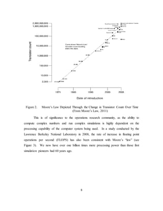
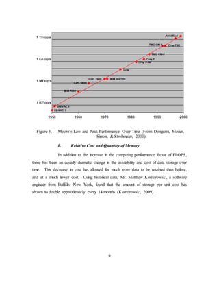
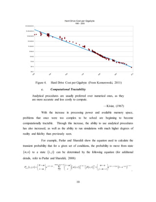
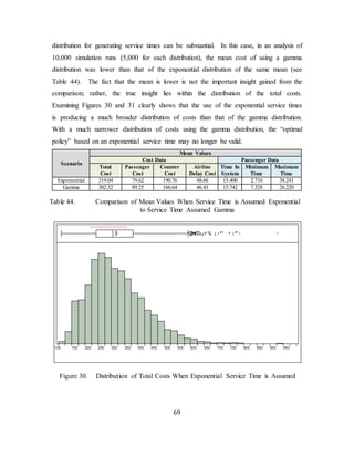
This thesis explores using simulation as a method of first resort for analyzing complex problems. It summarizes the development of computer simulation and its increasing usefulness due to advances in computing power. It then analyzes an airport check-in counter scheduling problem that was previously addressed through analytical methods. A simulation model of the problem is developed in Simio to compare results. The simulation is able to relax assumptions, consider more realistic distributions, and provide insights not possible through analysis alone. This demonstrates how simulation is often better suited than analysis for complex, real-world problems and supports changing the paradigm to use simulation as a primary analysis tool.


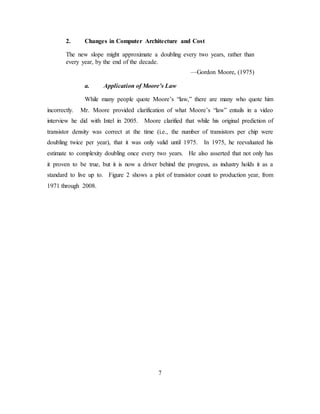
![2
From the Buffon needle experiments in the 1770s to estimate π, to the complex
models run on supercomputers and computing clusters today, simulation persists and has
grown in its use, but the phrase “as a last resort” can still be seen in scholarly papers.
One should examine how simulation has evolved over time in order to make the
determination if the adage is still valid.
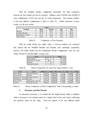
1. A Brief History of Computer Simulation
If you would understand anything, observe its beginning and its
development.
—Aristotle
Keeping with the academic spirit of Aristotle, let us examine the development of
simulation over time in order to gain an appreciation of the history of simulation and how
it has changed with the advances of technology. To examine the history of simulation,
Goldsman, Nance, and Wilson (2009) have provided a framework with which one can
segregate the changes of computing power over time and its effect on simulation. Their
framework consists of three definitive phases: the Precomputer Era (Pre–1945), the
Formative Period (1945–1970), and the Expansion Period (1970–1981). Their study of
simulation history stopped at 1981, as they did not believe that sufficient time had passed
to see any definitive changes since that time (James R. Wilson, personal communication,
August 11, 2011). However, during a discussion with Professor James Wilson of
North Carolina State University regarding the substantial increases in computing power
and memory availability, it was proposed that two additional periods may be examined:
the Maturation Period (1983–2000 [approximately]) and the Distributed Processing Era
(2000–present).
a. Precomputer Era
The idea behind the Monte Carlo approach. . . is to [replace] theory by
experiment whenever the former falters.
—Hammersley & Handscomb, (1964)
Although the term “Monte Carlo Simulation” was not known or discussed
at the time, the process we know today as “Monte Carlo Simulation” has been utilized as](https://image.slidesharecdn.com/3a25bb0e-5fa8-4cea-92e2-98b55f0229d1-150531113425-lva1-app6891/85/11Sep_Anderson-28-320.jpg)
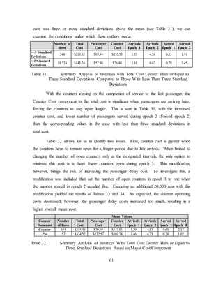
![5
that were not arbitrarily tied to a specific SPL and focused on computer simulation as a
method in general (e.g., Law & Kelton, 1982).
In addition to the improvement of SPLs, several other key topics were
advanced during this period. A new object-oriented approach to simulation design
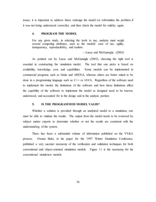
entitled “Conical Methodology” was developed by Nance (1978). Additionally, advances
in random number generation, event graphs (Schruben, 1983), and the need for formal
verification and validation (Blaci & Sargent, 1981) were brought forward. The text
Simulation Modeling and Analysis by Law and Kelton (1982) has been credited with
being the first of many that brought the advanced methodologies to a wide audience
(Goldsman, Nance, & Wilson, 2010).
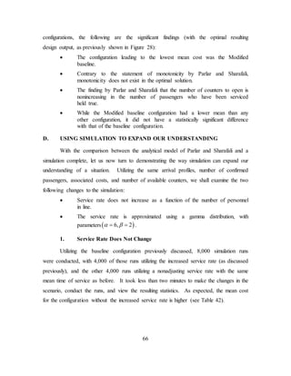
d. Maturation Period
With a definitive structure set in place on the issues that face the use of
simulation, combined with an ever increasing source of experts, research continued
throughout the maturation period on how one can achieve more reality and fidelity in
simulation. One source which has had a significant influence, and continues to underpin
these developments, is the Winter Simulation Conference (WSC).
While the WSC provides a forum for discussion of the most recent
advances in simulation, it also “provides the central meeting place for simulation
practitioners, researchers, and vendors working in all disciplines and in the industrial,
governmental, military, service, and academic sectors” (White, Fu, & Sanchez, 2011).
The WSC has annually brought together individuals and sponsors from six major
professional organizations and one government agency to accomplish this through a
completely volunteer lead effort for over 40 years (White, Fu, & Sanchez, 2011). For
more information on the WSC, and access to their past presentations and papers, refer to
http://wintersim.org/.
The Department of Defense’s (DoD) reliance on modeling and simulation
grew throughout the 1990s. It was during this period that the use of simulations for
operational wargaming became widespread (Army Modeling & Simulation Office
[AMSO], 2011). With that usage came the realization that without proper quality control](https://image.slidesharecdn.com/3a25bb0e-5fa8-4cea-92e2-98b55f0229d1-150531113425-lva1-app6891/85/11Sep_Anderson-31-320.jpg)
![17
d. Intelligence
M&S helps provide actionable events designed to stimulate/simulate the
proper human intelligence (HUMINT), signals intelligence (SIGINT), and geospatial
intelligence (GEOINT), which was gathered in real-world operations. M&S is also used
in training intelligence personnel for counterinsurgency operations.
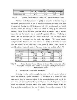
e. Testing
With changes in the DoD instruction for acquisition, M&S is required to
be used throughout a program’s life cycle (Office of the Under Secretary of Defense
(Acquisition, Technologies, and Logistics [OUSD-AT&L], 2006). This is done in order
to support requirements definition, the design and engineering phase, test planning,
rehearsal, and then the conduct of actual tests. It also is used to aid in evaluating the
performance of tested items, systems and/or organizations, and the early examination of
soldier interface and missions. Finally, simulation is used to help determine system
performance and safety. (For more information, refer to the Acquisition Modeling and
Simulation Master Plan available via the OUSD-AT&L website at:
www.acq.osd.mil/se/docs/AMSMP_041706_FINAL2.pdf.)
f. Training
M&S has been instrumental in preparing personnel for deployment to
recent combat operations through the significant growth of “the ability to link together
disparate virtual simulators and integrate constructive simulations to achieve complex
mission environments” (United States Air Force [USAF], 2010). Through the delivery of
integrated live, virtual, and constructive training environments that support personnel and
mission rehearsal requirements, predeployment training exercises, and mission
rehearsals, M&S has helped to ensure that personnel being deployed are trained and
ready. The United States Marine Corps has fully embraced the use of simulations in
training, and in an article on the Defense Transformation website (http://www.defense.
gov/transformation/), one article states:](https://image.slidesharecdn.com/3a25bb0e-5fa8-4cea-92e2-98b55f0229d1-150531113425-lva1-app6891/85/11Sep_Anderson-43-320.jpg)
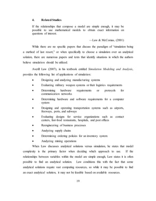
![21
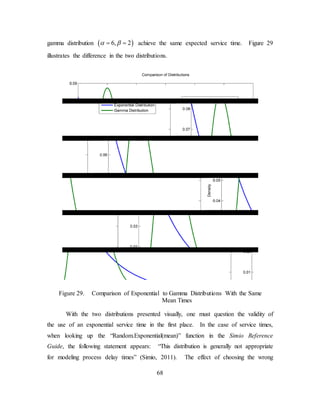
Of the advantages Professor Loerch states, two are extremely important in the
realm of military application of simulation. First, Professor Loerch (2001) states that
simulation is “not subject to so many assumptions.” Analytical solutions often require
multiple assumptions to be made in order to find a solution (e.g., normality,
independence, memorylessness, deterministic, linear, stationary, and homoscedasticity).
One distinct benefit of simulation is that one can often reduce the number of or change
the assumptions, which will allow for data outliers to enter the system. These outliers
may identify critical problems or shortfalls within the system that would never have been
seen using an analytical solution. Perhaps more importantly, Professor Loerch states that
simulation results are “easy for [a] decision maker to understand” (2001).
With the premise that “unplanned, hit-or-miss course of experimentation with a
simulation model can often be frustrating, inefficient, and ultimately unhelpful,” Kelton
(2000) provides a basic understanding on what is required in a simulation in order to
maximize the benefit from it in his paper “Experimental Design for Simulation.” This
paper, presented at the 2000 Winter Simulation Conference, discussesfive key
components that need to be addressed when developing a simulation:
• What model configuration should you run?
• How long should the run be?
• How many runs should you make?
• How should you interpret and analyze the output?
• What’s the most efficient way to make the runs?
Professor Kelton (2000) then continues to educate his readers on the importance
of utilizing carefully planned simulation studies to avoid “an undue amount of
computational effort or (more importantly) your time.”
B. RESEARCH QUESTIONS
This research seeks to answer the question as to when simulation should (and
should not) be used to gain insight into a problem. It further seeks to identify the benefits
one receives through a simulation approach to a problem, compared to the benefits of an
analytical solution to the same problem.](https://image.slidesharecdn.com/3a25bb0e-5fa8-4cea-92e2-98b55f0229d1-150531113425-lva1-app6891/85/11Sep_Anderson-47-320.jpg)

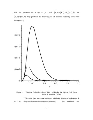
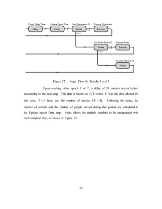
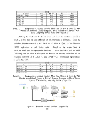
1 hrs.nτ τ< ⋅⋅⋅ <
ˆ
kλ
1 4 [0.32, 0.34, 0.42, 0.47] 0.31
2 6 [1.15, 1.46, 1.47, 1.58, 1.93, 1.96] 0.69
3 5 [2.11, 2.44, 2.57, 2.71, 2.87 1.83
Table 2. Numerical Example of Estimated Arrival Rates (From Parlar &
Sharafali, 2008)
Given that these arrival rates are constant over each 1-hour period, one would
expect that the projected number of arrivals would be able to be calculated. In this case,
there were 15 arrivals scheduled; however, using the calculated arrival rates, one cannot
match the expected number of arrivals with the number that actually arrived.
Finally, the authors assumed that all passengers arriving are traveling in the same
class. This is instrumental in their calculation of the passenger delay cost, as the cost is
set at a fixed value for all passengers. This, too, does not reflect the reality of most
airline traffic. It only applies when one is addressing a very minor number of instances
where there is no class differentiation on price of seat, or significance of the passengers.
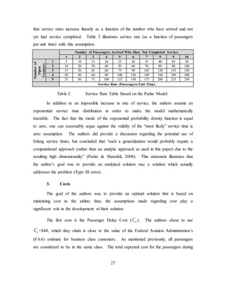
2. Service
The way in which the customers are served is the next set of assumptions that are
examined. First, over any given epoch, a constant number of counters are available. The
number of open counters can only change at the beginning of each period ( )k , which is
based on the number people who have arrived and the number of people who have
arrived and already completed service. The times at which these decisions are made are
based on the history of previous arrivals on which the arrival rates have already been
calculated. Thus far, the conditions set are not too unrealistic. However, when the
service rate is examined, it is another story. First, the authors assume that the service rate
for a given counter ( )µ is the same for each counter. Second, the service rate increases
as a function of the number of people who have not been served, and the number of open
counters. This presents a major issue with the analytical solution, as it is not reasonable](https://image.slidesharecdn.com/3a25bb0e-5fa8-4cea-92e2-98b55f0229d1-150531113425-lva1-app6891/85/11Sep_Anderson-52-320.jpg)


![[17-E-7]ComunityLT2011ご挨拶](https://cdn.slidesharecdn.com/ss_thumbnails/17-e-7comunityltse-110220015334-phpapp01-thumbnail.jpg?width=640&height=640&fit=bounds)