1. Proceedings of the 37th Hawaii International Conference on System Sciences - 2004
On Multiobjective Volt-VAR Optimization in Power Systems
Miroslav M. Begovic, Branislav Radibratovic, Frank C. Lambert
School of Electrical and Computer Engineering, Georgia Institute of Technology
Atlanta GA 30332-0250
miroslav@ece.gatech.edu
Abstract planning in transmission networks often addresses
transmission losses, transmission capacity and voltage
The need for simultaneous optimization of reactive stability as main objectives.
resources for the transmission and distribution system Various algorithms have been proposed to solve the
has long been recognized. If investment resources are capacitor placement problem, either on the transmission
limited, various combinations of solutions (voltage level, network or on the distribution feeders, when only one of
amount and type of reactive support, etc.) may impact a the above objectives is optimized. These types of
number of objectives (distribution losses, distribution problems are often referred to as single-objective
feeder power factor, voltage profile for conservative optimization problems. In recent years, multi-objective
voltage reduction, transmission losses, transmission problems have arisen in many engineering applications.
capacity, voltage stability, etc.). While solutions have Two or more objectives (usually confronted) need to be
been proposed for subsets of the above problems, few simultaneously optimized. The problem of simultaneous
algorithms have undertaken the simultaneous optimization of reactive resources on the transmission
optimization of reactive resources in the transmission and distribution system represents a further step in the
and distribution network. This paper attempts to address generalization of the problem. Only a few algorithms are
various issues that need to be solved: decomposition of applicable for simultaneous optimization of reactive
the transmission model from the distribution model, resources in the transmission and distribution network.
design of an interface suitable for simultaneous This paper addresses various issues that need to be
optimization, and development of the methodology solved: Decomposition of the transmission model from
(multiobjective optimization based on building Pareto the distribution model, design of the interface suitable
fronts with the help of custom-tailored genetic for simultaneous optimization and development of the
algorithms). Some of the issues discussed in this paper methodology (multiobjective optimization based the on
are illustrated on suitable examples and guidelines building of Pareto optimal solution fronts through the
proposed for building a practical model that would use of custom-tailored genetic algorithms).
incorporate all of the concerns with the modeling issues.
2. Concept of multi-objective optimization
Index Terms—volt/var optimization in power
systems, multiobjective optimization. In many practical problems, several optimization
criteria need to be satisfied simultaneously. Moreover, it
1. Introduction is often not advisable to combine them into a single
objective. While it may sometimes happen that a single
Modern electric utility companies are faced with the solution optimizes all of the criteria, the more likely
problem of constant load growth together with a strict scenario is when one solution is optimal with respect to
limitation of investment resources, which severely limits a single criterion while other solutions are best with
the growth of the infrastructure. One method for respect to the other criteria. The increase of the
increasing transmission capacity is investment in “goodness” of the solution with respect to one objective
reactive resources, which are used in both transmission will produce a decrease of its “goodness” with respect to
and distribution networks. While locating and sizing the others. While there are no problems in understanding
reactive support, different objectives can be chosen. the notion of optimality in single objective problems,
Design goals in distribution networks are usually multiobjective optimization requires the concept of
optimization of distribution losses, distribution feeder Pareto-optimality.
power factor and voltage profile. Reactive power
0-7695-2056-1/04 $17.00 (C) 2004 IEEE 1

2. Proceedings of the 37th Hawaii International Conference on System Sciences - 2004
The solution is said to be Pareto-optimal (belongs to 3. Test model
the Pareto-optimal front, or set of solutions) if, with its
change not one objective function can be improved Any attempt to solve the multiobjective Volt-Var
without degrading all of the others. All of the solutions optimization for the entire power system will present a
that make up a Pareto-optimal front are said to be non- monumental challenge due to the system size and
dominated (by other solutions). Concepts of the Pareto- complexity of the solution. To that end, it is proposed to
optimal front, non-dominated and dominated solutions decouple the transmission model from the distribution
are further explained in Fig. 1. The axes on Fig. 1 (F1 model. The transmission system and each distribution
and F2) are two objective functions. Possible solutions feeder can be investigated separately. The Pareto-
for minimization are presented in the F1-F2 plane. optimal front of the solutions is found for every
Solutions marked with triangles are called non- distribution feeder and the transmission system as well.
dominated and they make up the Pareto-optimal front. These solutions then provide input data to a suitably
Those marked with circles are the dominated (non- designed interface algorithm. The design of the interface
Pareto optimal) solutions. algorithm capable of finding the globally optimal
solution is the main goal of this research. The algorithm
F2 should solve for the Pareto optima while simultaneously
taking into consideration both transmission system and
Dominated solution distribution feeder solutions.
x3
As an illustration of the system decomposition,
x1 Non-dominated solution transmission and distribution system models are shown
in Fig. 2 and Fig. 3, respectively. These models will be
x2 used as an instructional example for the proposed
algorithm. The transmission model is derived from the
Pareto-optimal IEEE 5-bus system by removing the second generator
front originally connected to bus 3. This alteration is made to
enable two possible alternatives for capacitor placement
on the transmission network, namely bus 1 and bus 3.
F1 The distribution feeder model is derived from the
IEEE 13-node test feeder. This feeder is very small but
relatively highly loaded, which enables various
Fig. 1. Pareto-optimality, non-dominated and
possibilities for capacitor placement. The following
dominated solutions, bi-objective case
modifications are performed on the original feeder: The
existing switch and low voltage transformer are
A solution x is dominated if there exists a solution y
removed from the model, the distributed load is
such that for all objective functions Fi stands:
neglected, and all loads have been balanced. Table 1
Fi(x) ≤ Fi(y) for all i ∈ {1,2,…, n} summarizes the necessary feeder data.
If the solution is not dominated by any other feasible 4 2 3
solution, we call it a non-dominated (Pareto-optimal)
solution. If the domination operator is “ ”:
G
• x1 x3 and x2 x3 (x3 is dominated) P3,
• x1 x2 and x2 x1 (x1, x2 are non-dominated) Q3
1
P1, Q1
Fig. 2. Transmission system model
0-7695-2056-1/04 $17.00 (C) 2004 IEEE 2

3. Proceedings of the 37th Hawaii International Conference on System Sciences - 2004
TS Optimize: F
0
Subject to: G( , V, Qc) = 0 (1)
Qci = k Qc0 k = 0, 1, 2 …
where:
4 3 1 2 F - vector of objectives
G - set of power flow equations
- vector of voltage angles
V - vector of voltage magnitudes
10 8 5 6 Qc- vector of reactive support
Qci - reactive support applied to the bus “i”
Qc0 - incremental reactive support step
4.1. Distribution system
9 7
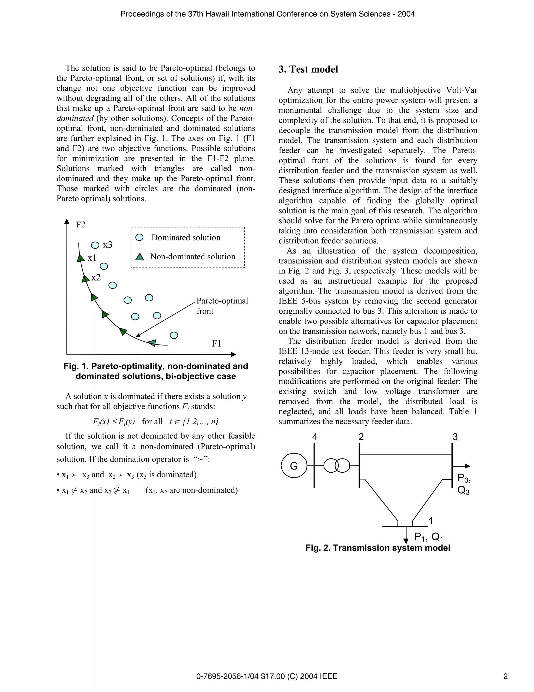
Fig. 3. Distribution feeder model This section presents Pareto-optimal solutions for the
feeder shown in Fig. 3. Solving for any Pareto-optimal
Table 1. Feeder load data front assumes more than one objective. Two
(confronted) objectives chosen here are: 1) the
Node P (kW) Q (kVAr) investment in reactive resources (assumed to be directly
2 400 290 proportional to the amount of reactive support); and 2)
3 170 125 feeder losses. The optimization problem (1) therefore
4 230 132 can then be reformulated as:
5 1155 660
6 1013 613 Minimize: Ploss = Ploss ( , V, Qc)
9 126 86 11
10 170 80 Minimize: Investment = Qci ⋅ PF
i =1 (2)
To link the distribution feeder models with the Subject to: G( , V, Qc) = 0;
transmission network, all of the feeder loads are doubled Qci = k Qc0 k = 0, 1, 2 …
and it is assumed that ten identical feeders are connected where:
to each transmission load bus (bus 1 and bus 3). The set PF - price of capacitor on the distribution feeder
of feeders on each transmission bus represents a model
of the distribution system. 4.1.1. Genetic algorithm as an optimization tool.
There are several ways to solve the optimization
4. Optimization algorithm problem (2). Genetic algorithms (GAs) are the natural
tool for solving the problem, even more so when other
The general approach for solution of the multi- objectives are also included in the optimization. As
objective Volt-Var problem requires that reactive described in [1], “Genetic algorithms are based on the
resources be divided between the transmission and mechanics of natural selection and natural genetics”. GA
distribution system. The list of optimization objectives differs from traditional (calculus-based) optimization
may include distribution losses, distribution feeder and search procedures in following ways:
power factor, voltage profile, transmission losses, • It uses probabilistic transition rules rather than the
transmission capacity, voltage stability, etc. deterministic ones.
We propose that the power system model be separated • It does not need the knowledge of gradients or any
into transmission and distribution subsystems. These other auxiliary knowledge of the objective function.
systems are to be solved separately. Families of It uses only the objective function values, evaluated
solutions for capacitor placement are found for each at a number of points.
subsystem. These solutions should then be combined • It works with a population of solutions rather than
with a suitably designed interface algorithm to filter the with a single solution.
unique Pareto-optimal solution front. The optimization For the solution of the problem defined in (2), bi-
problem for both systems, treated separately, can be objective GA is applied. The cost of the feeder reactive
formulated as: support is assumed to be Pf = 15 $/kVA. The incremental
reactive support step is assumed to be Qc0 = 100
0-7695-2056-1/04 $17.00 (C) 2004 IEEE 3

4. Proceedings of the 37th Hawaii International Conference on System Sciences - 2004
kVA/phase. The optimization results are presented in This problem can be solved using the same genetic
Fig. 5 and Table 2. Figure 5 shows the Pareto-optimal algorithm as the distribution feeder. The cost of the
front of the solutions, while Table 2 provides numerical transmission reactive support is assumed to be PT =
explanations for only a few of the possible solutions. 10 $/kVA. The incremental reactive support step is
Due to the linear relationship between investment and assumed to be Qc0 = 1 MVA/phase. The optimization
the amount of reactive support, the latter is shown as an results are presented in Fig. 6 and Table 3. Figure 6
objective in Fig. 5. shows the transmission system Pareto-optimal front of
solutions, while Table 3 provides numerical
6
explanations for a few of the possible solutions. Due to
the linear dependence between investment and the
5 amount of reactive support, the latter is shown as an
objective in Fig. 6.
Rea ctive supp ort (M V A )
4
90
80
3
70
Reactive support (M V A )
2
60
50
1
40
0
270 290 310 330 350 370 390 410 430 450 470 30
D istrib utio n lo sses (kW )
20
Fig. 5. Distribution feeder, Pareto-optimal front
of solutions (every point represents a different 10
capacitor allocation on the feeder) 0
6 7 8 9 10 11 12 13 14
Transm ission Losses (M W )
Table 2. A few of the distribution feeder Pareto-
Fig. 6. Transmission system, Pareto-optimal
optimal solutions
front
C1 C2 C3 C4 C5 C6 C9 ΣC Ploss
MVA MVA MVA MVA MVA MVA MVA MVA kW Table 3. Structure of transmission system
0 0 0 0 0 0.3 0 0.3 466 Pareto-optimal solutions
0 0 0 0 0 1.5 0.3 1.8 367
0 0 0 0 1.2 1.5 0.3 3.0 315 C1 (MVA) 0 2 11 18 25 31 42
0 0.6 0.3 0.3 1.8 1.5 0.3 4.8 280 C3 (MVA) 10 28 29 32 35 39 44
0.9 0.6 0.3 0.3 1.8 1.5 0.3 5.7 277 ΣC (MVA) 10 30 40 50 60 70 86
Ploss (MW) 12.3 9.7 8.69 7.86 7.20 6.73 6.43
4.2. Transmission system
4.3. Interface algorithm
The transmission system should be solved separately
from the distribution system. Transmission losses and The main challenge is how to optimize reactive
the amount of reactive support are the two selected resources, with respect to multiple criteria, for the entire
minimization criteria. The optimization problem (1), transmission and distribution system. Defining system
applied on transmission system model shown in Fig. 2, losses as the optimization objective, the optimization
can be reformulated as: problem can be cast as:
Minimize: Ploss = Ploss ( , V, Qc) Minimize: ΣPloss = Ploss,TS + ΣPloss,F
2
Minimize: Investment = Qci ⋅ PT (3) Subject to: G( , V, Qc) = 0;
i =1 Qci = k Qc0T (4)
Subject to: G( , V, Qc) = 0; Qcj = k Qc0F
Qci = k Qc0 k = 0, 1, 2 … PT ⋅ Qci + PF ⋅ Qcj ≤ I .R.
i j
0-7695-2056-1/04 $17.00 (C) 2004 IEEE 4

5. Proceedings of the 37th Hawaii International Conference on System Sciences - 2004
where: Step 8. Extract optimal solution.
ΣPloss,F - sum of losses of all feeders in system
k - non-negative integer 4.3.2. Application of Interface Algorithm to the Test
Qci - reactive support applied at transmission bus System. In the following example, the limit for
“i” investment resources is chosen to correspond to the top
Qcj - reactive support applied at feeder node “j” point of the transmission system Pareto front. It amounts
Qc0T - transmission incremental reactive support to $860,000 (10$/kVA*86MVA). To further reduce the
step complexity of the problem, it is assumed that the voltage
Qc0F - feeder incremental reactive support step on the source end of the feeders (node 0) is kept
I.R. - limitation of investment resources constant, which further decouples the problem. In this
way, the feeder consumption (P and Q loads at
In the optimization problem (4), the questions to be transmissions buses), together with feeder losses, is kept
answered are: dependent only on the amount of reactive support
• How to allocate resources in both the transmission applied on the feeder. The feeder consumption is not
and distribution networks. dependent on voltages at transmission buses; i.e. it is not
• How to divide the resources between networks. dependent on transmission capacitor allocation.
• How to divide the support between feeders The above algorithm produces the set of solutions
connected to different transmission buses. depicted in Fig. 7. It represents overall losses as a
The first question is already answered with the Pareto function of the transmission reactive support (in MVA
fronts of Fig. 5 and Fig. 6. The answers to the or in dollar terms). Investment resources are kept
subsequent questions will be provided by the interface constant. The difference in reactive support between the
algorithm. The interface algorithm combines both Pareto initial solution (86MVA) and any subsequent point is
fronts and finds particular solutions that represent a transferred as support to the distribution feeders. The
global optimum. graph in Fig. 7 contains 19 sets of solutions
corresponding to 19 possible scenarios of feeder
4.3.1. Algorithm structure. compensation (19 members of the feeder Pareto-optimal
Step 1. Choose an initial solution. front).
Find a transmission Pareto solution (Fig. 6) that 90
corresponds to a certain amount of investment (reactive
support). If the investment resources are higher than the 80
Tra nsm issio n re a ctive sup po rt (M V A )
investment corresponding to the top point in the Pareto 70
front, choose the top point as the starting point (keeping
in mind that additional investment should be available 60
for the distribution system). 50
Step 2. Outer loop starts.
Starting from the initial solution, go down the 40
transmission Pareto front. Repeat the following steps for 30
each transmission solution.
20
Step 3. Calculate the available feeder support (reactive
resources). 10
Step 4. Inner loop starts.
0
Compensate the feeders at each transmission bus with 14 14.5 15 15.5 16 16.5
the available reactive support. Ove ra ll lo sse s (MW )
Step 5. Find the optimal capacitor allocation for the Fig. 7. Overall losses vs. level of transmission
feeder(s). reactive support (investment resources limited
Use sensitivity analysis of losses with respect to the at $860,000)
active and reactive load on the transmission buses with
compensated feeders and find the optimal feeder The minimal overall losses correspond to the solution
schedule (number of compensated feeders on a when only 14 MVA is applied in the transmission
particular transmission bus). Reduce the reactive support system. The following capacitor placement scenario
from the transmission bus that is the most insensitive to yields the minimal losses:
the losses and transfer that support to the most sensitive
bus. Transmission system: C1 = 0 C2 = 14MVA
Step 6. Inner loop ends. Distribution feeder: C2=0.6MVA C3=0.3MVA
Step 7. Outer loop starts. C4=0.3MVA C5=1.8MVA C6=1.5MVA C9=0.3MVA
0-7695-2056-1/04 $17.00 (C) 2004 IEEE 5

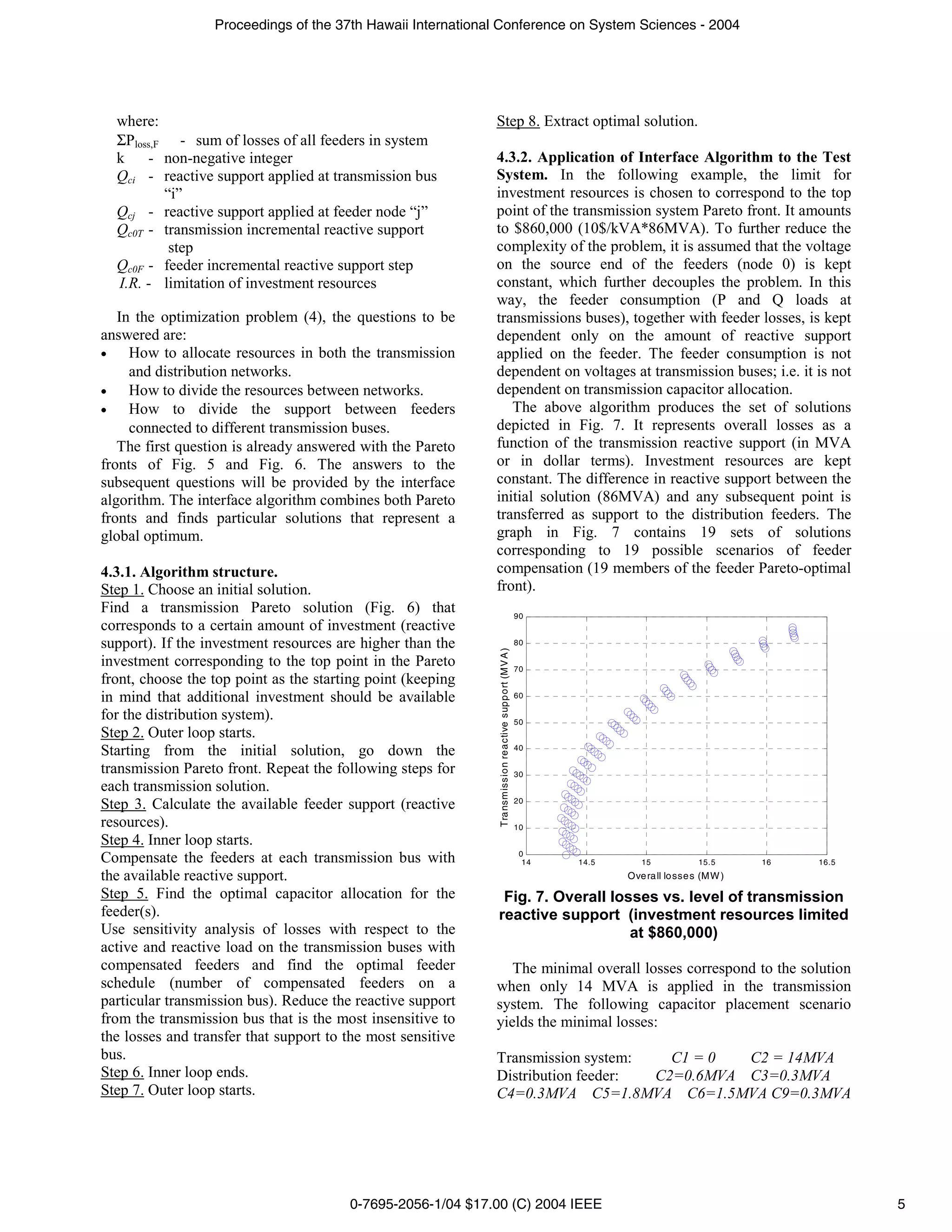
6. Proceedings of the 37th Hawaii International Conference on System Sciences - 2004
Optimal feeder schedule: BUS1 - 50%, BUS3 - 50% initial solution (86MVA support
1.1 to transmission system)
no reactive support
The transmission system was supported with 14MVA, 1 solution that minimizes loses
while the overall feeder support was 48MVA (ten
0.9
feeders compensated with 4.8MVA each). The fact that
V oltage at bus 3 (p.u.)
the distribution feeders require 77% of the overall 0.8
reactive support is because of their high load and
0.7
extremely bad power factor. The best solution yields an
overall loss ΣPloss= 4.29MVA, which is 12% less than 0.6
the initial solution (16.21MVA), and still requires the
0.5
same investment. (14MVA*$10/kVA +
10feeders*4.8MVA*$15/kVA = $860,000) 0.4
0.3
5. Impact on voltage stability margin
0.2
1 1.1 1.2 1.3 1.4 1.5
The influence of the capacitor allocations discussed in Loading factor (p.u.)
the above example on the voltage stability margin is Fig. 8. System’s PV curves for different
investigated. Continuation power flow, applied on the capacitor scenarios
system model without reactive support, yields some
alarming data. The critical loading factor of the system Decomposition of the transmission model from the
is λ = 1.108 (10.8 percent load increase before voltage distribution feeders is proposed as a necessary step to
collapse). Applying reactive support to the system is reduce the complexity of the problem. After the
expected to be beneficial, but it is not known whether decoupled parts of the system are solved independently,
the transfer of reactive support from the transmission to a suitable interface is designed for simultaneous
the distribution portion of the system would worsen the optimization. Custom designed genetic algorithms are
voltage stability loading margin. The answer appears to used as multiobjective optimization tools that rely on
be negative. Transferring reactive support to the sensitivity analysis to reduce the search space and allow
distribution network decreases the reactive load of the implementation for large system models.
transmission system and increases the system voltage
stability loading margin. Figure 8 illustrates this 7. Acknowledgment
observation. The following PV curves are shown in
Fig.8: Financial support of the National Electric Energy
• No reactive support to system (λ = 1.108) Testing, Research and Applications Center (NEETRAC)
• Entire ($860k) reactive support applied to the used for part of the work presented in this paper is
transmission network (critical loading margin gratefully acknowledged. The authors also would like to
increased to λ=1.294) acknowledge Dr. Damir Novosel, with whom they had
• Minimal loss scenario (critical loading margin many fruitful discussions about multi-objective
further increased to λ=1.508) optimizations.
6. Conclusions 8. References
The problem of simultaneous optimization of reactive [1] D Goldberg, Genetic Algorithm in Search, Optimization
resources on the transmission and distribution system is and Machine Learning, New York: Addison Wesley,
solved by decoupling the analysis of the transmission 1989.
and distribution networks. The investment resources are [2] B. Baran, J. Vallejos, R. Ramos, U. Fernandez "Reactive
assumed to be limited and known. Under this Power Compensation using a Multi-objective
constraint, a number of optimization objectives can be Evolutionary Algorithm" IEEE Porto Power Tech
chosen (distribution losses, distribution feeder power Conference, Porto, Portugal September, 2001
[3] J.T. Ma, L.L. Lai “Evolutionary Programming Approach
factor, voltage profile for conservative voltage
to Reactive Power Planning” IEE Proceedings –
reduction, transmission losses, transmission capacity, Generation, Transmission and Distribution, Vol 143, No.
voltage stability, etc.). This paper addresses the various 4, July 1996
issues that need to be resolved to solve this problem.
0-7695-2056-1/04 $17.00 (C) 2004 IEEE 6