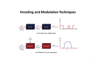
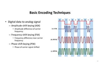
300952
Wireless and Mobile
Networks
Lecture 5. Signal Encoding Techniques
Lecture objectives
• Understand the reasons for using encoding techniques
• Compare and select encoding techniques
• Understand the three main ways digital data can be encoded in analog signals
• Understand methods to modulate analog data in analog and digital signals
2
INTRODUCTION
3
Review from Lecture 2
• Analog signal: signal intensity varies in a smooth fashion over time
– No breaks or discontinuities in the signal
• Digital signal: signal intensity maintains a constant level for some
period of time and then changes to another constant level
4
Encoding and Modulation Techniques
5
Reasons for Choosing Encoding Techniques
• Digital data, digital signal
– Equipment less complex and expensive than digital-to-analog modulation
equipment
• Analog data, digital signal
– Permits use of modern digital transmission and switching equipment
• Digital data, analog signal
– Some transmission media will only propagate analog signals
– E.g., optical fiber and unguided media
• Analog data, analog signal
– Analog data in electrical form can be transmitted easily and cheaply
– Done with voice transmission over voice-grade lines
6
Signal Encoding Criteria
• What determines how successful a receiver will be in interpreting an
incoming signal?
– Signal-to-noise ratio (SNR)
– Data rate
– Bandwidth
• An increase in data rate increases bit error rate
• An increase in SNR decreases bit error rate
• An increase in bandwidth allows an increase in data rate
7
Factors Used to Compare Encoding Schemes
• Signal spectrum
– With lack of high-frequency components, less bandwidth required
– With no DC component, AC coupling via transformer is possible
– Transfer function of a channel is worse near band edges
• Clocking
– Ease of determining beginning and end of each bit position
• Signal interference and noise immunity
– Performance in the presence of noise
• Cost and complexity
– The higher the signal rate to achieve a given data rate, the greater the cost
8
DIGITAL DATA, ANALOG SIGNALS
9
Basic Encoding Techniques
• Digital data to analog signal
– Amplitude-shift keying (ASK)
• Amplitude difference of carrier
frequency
– Frequency-shift keying (FSK)
• Frequency difference near carrier
frequency
– Phase-shift keying (PSK)
• Phase of carrier signal shifted
10
Amplitude-Shift Keying (1)
• One binary digit represented by presence of carrier, at constant amplitude
• Other binary digit represented by absence of carrier
• where the carrier signal is Acos(2πfct)
• Susceptible to sudden gain changes
• Inefficient modulation technique
• Used to transmit digital data over optical fiber
11
( )





=
t
s
Acos 2p fc
t
( )
0
1
binary
0
binary
Digitizing Analog Data
12
Binary Frequency-Shift Keying (BFSK)
• Two binary digits represented by two different frequencies near the
carrier frequency
• where f1 and f2 are offset from carrier frequency fc by equal but opposite amounts fd
• Less susceptible to error than ASK
• Used for high-frequency (3 to 30 MHz) radio transmission
• Can be used at higher frequencies on LANs that use coaxial cable
13
( )





=
t
s
Acos 2p f1
t
( )
Acos 2p f2
t
( )
1
binary
0
binary
Full-Duplex FSK Transmission on a Voice Grade Channel
14
Multiple Frequency-Shift Keying (MFSK) (1)
• More than two frequencies are used
• More bandwidth efficient but more susceptible to error
• f i = f c + (2i – 1 – M)f d
• f c = the carrier frequency
• f d = the difference frequency
• M = number of different signal elements = 2L
• L = number of bits per signal element
15
si
t
( )= Acos2p fi
t 1£i £ M
Multiple Frequency-Shift Keying (MFSK) (2)
• To match data rate of input bit stream, each output signal element is held for:
Ts=LT seconds
• where T is the bit period (data rate = 1/T)
• So, one signal element encodes L bits
• Total bandwidth required
2Mfd
• Minimum frequency separation required
• 2fd=1/Ts
• Therefore, modulator requires a bandwidth of
Wd=2L/LT=M/Ts
16
Phase-Shift Keying (PSK) (1)
• Two-level PSK (BPSK)
– Uses two phases to represent binary digits
– Used in IEEE 802.11a
17
( )





=
t
s
Acos 2p fc
t
( )
Acos 2p fc
t +p
( )
1
binary
0
binary





=
Acos 2p fc
t
( )
-Acos 2p fc
t
( )
1
binary
0
binary
Phase-Shift Keying (PSK) (2)
• Differential PSK (DPSK)
– Phase shift with reference to previous bit
• Binary 0 – signal burst of same phase as previous signal burst
• Binary 1 – signal burst of opposite phase to previous signal burst
18
Quadrature Phase-Shift Keying (PSK)
• Four-level PSK (QPSK)
– Each element represents more than one bit
– Used in IEEE 802.11a
19
s(t)=
ì
í
ï
î
ï
Acos 2p fc
t +
p
4
æ
è
ç
ö
ø
÷ 11
Acos 2p fc
t +
3p
4
æ
è
ç
ö
ø
÷
Acos 2p fc
t -
3p
4
æ
è
ç
ö
ø
÷
Acos 2p fc
t -
p
4
æ
è
ç
ö
ø
÷
01
00
10
QPSK Constellation Diagram
20
Multilevel PSK
• Using multiple phase angles with each angle having more than one
amplitude, multiple signal elements can be achieved
– D = modulation rate, baud or symbols/sec
– R = data rate, bps
– M = number of different signal elements = 2L
– L = number of bits per signal element
21
M
R
L
R
D
2
log
=
=
Performance (1)
• Bandwidth of modulated signal (BT)
– ASK, PSK BT = (1+r)R
– FSK BT = 2Δf+(1+r)R
• R = bit rate
• 0 < r < 1; related to how signal is filtered
• Δf = f2 – fc = fc - f1
22
Performance (2)
• Bandwidth of modulated signal (BT)
– MPSK
– MFSK
• L = number of bits encoded per signal element
• M = number of different signal elements
23
R
M
r
R
L
r
BT 






 +
=





 +
=
2
log
1
1
( ) R
M
M
r
BT 






 +
=
2
log
1
Quadrature Amplitude Modulation
• QAM is a combination of ASK and PSK
– Two different signals sent simultaneously on the same carrier frequency
24
s t
( )= I t
( )cos2p fc
t +Q t
( )sin2p fc
t
16QAM Constellation Diagram
25
Used in IEEE 802.11a
ANALOG DATA, ANALOG SIGNALS
26
Reasons for Analog Modulation
• Modulation of digital signals
– When only analog transmission facilities are available, digital to analog
conversion required
• Modulation of analog signals
– A higher frequency may be needed for effective transmission
– Modulation permits frequency division multiplexing
27
Basic Encoding Techniques
• Analog data to analog signal
– Amplitude modulation (AM)
– Angle modulation
• Frequency modulation (FM)
• Phase modulation (PM)
28
Amplitude Modulation (1)
• Amplitude Modulation
• cos2πfct = carrier
• x(t) = input signal
• na = modulation index
– Ratio of amplitude of input signal to carrier
– a.k.a double sideband transmitted carrier (DSBTC)
29
s t
( )= 1+na
x t
( )
é
ë
ù
ûcos2p fc
t
Amplitude Modulation (2)
30
Amplitude Modulation (3)
31
Single Sideband (SSB)
• Variant of AM is single sideband (SSB)
– Sends only one sideband
– Eliminates other sideband and carrier
• Advantages
– Only half the bandwidth is required
– Less power is required
• Disadvantages
– Suppressed carrier cannot be used for synchronization purposes
32
Angle Modulation (1)
• Angle modulation
• Phase modulation
– Phase is proportional to modulating signal
• np = phase modulation index
33
s t
( )= Ac
cos 2p fc
t +j t
( )
é
ë
ù
û
( ) ( )
t
m
n
t p
=

Angle Modulation (2)
• Frequency modulation
– Derivative of the phase is proportional to the modulating signal
• nf = frequency modulation index
34
j' t
( )= nf
m t
( )
Amplitude, Phase, and Frequency Modulation of a Sine-Wave
Carrier by a Sine-Wave Signal
35
Angle Modulation (3)
• Compared to AM, FM and PM result in a signal whose bandwidth:
– is also centered at fc
– but has a magnitude that is much different
• Angle modulation includes which produces a wide range of frequencies
• Thus, FM and PM require greater bandwidth than AM
36
cos j(t)
( )
ANALOG DATA, DIGITAL SIGNALS
37
Basic Encoding Techniques
• Analog data to digital signal
– Pulse code modulation (PCM)
– Delta modulation (DM)
38
Pulse Code Modulation
• Based on the sampling theorem
• Each analog sample is assigned a binary code
– Analog samples are referred to as pulse amplitude modulation (PAM) samples
• The digital signal consists of block of n bits, where each n-bit number is
the amplitude of a PCM pulse
• By quantizing the PAM pulse, original signal is only approximated
• Leads to quantizing noise
39
Pulse Code Modulation Example
40
Analog Data to Digital Signal
• Once analog data have been converted to digital signals, the digital data:
– can be transmitted using NRZ-L
– can be encoded as a digital signal using a code other than NRZ-L
– can be converted to an analog signal, using previously discussed techniques
41
Delta Modulation (1)
• Analog input is approximated by staircase function
– Moves up or down by one quantization level (d in the figure on next slide) at
each sampling interval
• The bit stream approximates derivative of analog signal (rather than
amplitude)
– 1 is generated if function goes up
– 0 otherwise
42
Example of Delta Modulation
43
Delta Modulation (2)
• Two important parameters
– Size of step assigned to each binary digit
– Sampling rate
• Accuracy improved by increasing sampling rate
– However, this increases the data rate
• Advantage of DM over PCM is the simplicity of its implementation
44
Reasons for Growth of Digital Techniques
• Growth in popularity of digital techniques for sending analog data
– Repeaters are used instead of amplifiers
• No additive noise
– TDM is used instead of FDM
• No intermodulation noise
– Conversion to digital signaling allows use of more efficient digital switching
techniques
45
Model-based encoding and Vocoders
• PCM and DM are types of waveform encoders
– Seek to reproduce the sampled waveform
• The nature of the signal can also be encoded
– For example, voice has particular characteristics
– Pitch
– Voiced sounds – m, n, b, etc.
– Unvoiced sounds – c, k, t, etc.
46
Model-based encoding and Vocoders
• Linear Prediction Coding (LPC)
– Estimate how the voice is producing the sound
• Code-excited Linear Prediction (CELP)
– Create a codebook of typical LPC results
– Transmit a digital signal of codebook indices
• If the codebook is small, the data rate of the signal can be quite small
• But larger codebooks produce better quality results since they match the voice more
precisely
• LPC and CELP coders can produce rates of 1.2 kbps to 13 kbps
47
VIDEO CODING
• Video compression
– Pictures may not change much frame-to-frame
• So, just mainly encode the differences instead of the entire images
– There may be redundancy inside each image as well
• These redundant elements can be encoded as repetitions
• Video can be compressed down to 1-3 Mbps, even down to 64 kbps
48
Sources for this lecture
Cory Beard, William Stallings. Wireless Communication Networks and
Systems, 1st edition. Pearson Higher Education, 2016
(Chapter 7)
All material copyright 2016
Cory Beard and William Stallings, All rights reserved
49

05_Signal_Encoding_Techniques.pdf

  • 1.
    300952 Wireless and Mobile Networks Lecture5. Signal Encoding Techniques
  • 2.
    Lecture objectives • Understandthe reasons for using encoding techniques • Compare and select encoding techniques • Understand the three main ways digital data can be encoded in analog signals • Understand methods to modulate analog data in analog and digital signals 2
  • 3.
  • 4.
    Review from Lecture2 • Analog signal: signal intensity varies in a smooth fashion over time – No breaks or discontinuities in the signal • Digital signal: signal intensity maintains a constant level for some period of time and then changes to another constant level 4
  • 5.
  • 6.
    Reasons for ChoosingEncoding Techniques • Digital data, digital signal – Equipment less complex and expensive than digital-to-analog modulation equipment • Analog data, digital signal – Permits use of modern digital transmission and switching equipment • Digital data, analog signal – Some transmission media will only propagate analog signals – E.g., optical fiber and unguided media • Analog data, analog signal – Analog data in electrical form can be transmitted easily and cheaply – Done with voice transmission over voice-grade lines 6
  • 7.
    Signal Encoding Criteria •What determines how successful a receiver will be in interpreting an incoming signal? – Signal-to-noise ratio (SNR) – Data rate – Bandwidth • An increase in data rate increases bit error rate • An increase in SNR decreases bit error rate • An increase in bandwidth allows an increase in data rate 7
  • 8.
    Factors Used toCompare Encoding Schemes • Signal spectrum – With lack of high-frequency components, less bandwidth required – With no DC component, AC coupling via transformer is possible – Transfer function of a channel is worse near band edges • Clocking – Ease of determining beginning and end of each bit position • Signal interference and noise immunity – Performance in the presence of noise • Cost and complexity – The higher the signal rate to achieve a given data rate, the greater the cost 8
  • 9.
  • 10.
    Basic Encoding Techniques •Digital data to analog signal – Amplitude-shift keying (ASK) • Amplitude difference of carrier frequency – Frequency-shift keying (FSK) • Frequency difference near carrier frequency – Phase-shift keying (PSK) • Phase of carrier signal shifted 10
  • 11.
    Amplitude-Shift Keying (1) •One binary digit represented by presence of carrier, at constant amplitude • Other binary digit represented by absence of carrier • where the carrier signal is Acos(2πfct) • Susceptible to sudden gain changes • Inefficient modulation technique • Used to transmit digital data over optical fiber 11 ( )      = t s Acos 2p fc t ( ) 0 1 binary 0 binary
  • 12.
  • 13.
    Binary Frequency-Shift Keying(BFSK) • Two binary digits represented by two different frequencies near the carrier frequency • where f1 and f2 are offset from carrier frequency fc by equal but opposite amounts fd • Less susceptible to error than ASK • Used for high-frequency (3 to 30 MHz) radio transmission • Can be used at higher frequencies on LANs that use coaxial cable 13 ( )      = t s Acos 2p f1 t ( ) Acos 2p f2 t ( ) 1 binary 0 binary
  • 14.
    Full-Duplex FSK Transmissionon a Voice Grade Channel 14
  • 15.
    Multiple Frequency-Shift Keying(MFSK) (1) • More than two frequencies are used • More bandwidth efficient but more susceptible to error • f i = f c + (2i – 1 – M)f d • f c = the carrier frequency • f d = the difference frequency • M = number of different signal elements = 2L • L = number of bits per signal element 15 si t ( )= Acos2p fi t 1£i £ M
  • 16.
    Multiple Frequency-Shift Keying(MFSK) (2) • To match data rate of input bit stream, each output signal element is held for: Ts=LT seconds • where T is the bit period (data rate = 1/T) • So, one signal element encodes L bits • Total bandwidth required 2Mfd • Minimum frequency separation required • 2fd=1/Ts • Therefore, modulator requires a bandwidth of Wd=2L/LT=M/Ts 16
  • 17.
    Phase-Shift Keying (PSK)(1) • Two-level PSK (BPSK) – Uses two phases to represent binary digits – Used in IEEE 802.11a 17 ( )      = t s Acos 2p fc t ( ) Acos 2p fc t +p ( ) 1 binary 0 binary      = Acos 2p fc t ( ) -Acos 2p fc t ( ) 1 binary 0 binary
  • 18.
    Phase-Shift Keying (PSK)(2) • Differential PSK (DPSK) – Phase shift with reference to previous bit • Binary 0 – signal burst of same phase as previous signal burst • Binary 1 – signal burst of opposite phase to previous signal burst 18
  • 19.
    Quadrature Phase-Shift Keying(PSK) • Four-level PSK (QPSK) – Each element represents more than one bit – Used in IEEE 802.11a 19 s(t)= ì í ï î ï Acos 2p fc t + p 4 æ è ç ö ø ÷ 11 Acos 2p fc t + 3p 4 æ è ç ö ø ÷ Acos 2p fc t - 3p 4 æ è ç ö ø ÷ Acos 2p fc t - p 4 æ è ç ö ø ÷ 01 00 10
  • 20.
  • 21.
    Multilevel PSK • Usingmultiple phase angles with each angle having more than one amplitude, multiple signal elements can be achieved – D = modulation rate, baud or symbols/sec – R = data rate, bps – M = number of different signal elements = 2L – L = number of bits per signal element 21 M R L R D 2 log = =
  • 22.
    Performance (1) • Bandwidthof modulated signal (BT) – ASK, PSK BT = (1+r)R – FSK BT = 2Δf+(1+r)R • R = bit rate • 0 < r < 1; related to how signal is filtered • Δf = f2 – fc = fc - f1 22
  • 23.
    Performance (2) • Bandwidthof modulated signal (BT) – MPSK – MFSK • L = number of bits encoded per signal element • M = number of different signal elements 23 R M r R L r BT         + =       + = 2 log 1 1 ( ) R M M r BT         + = 2 log 1
  • 24.
    Quadrature Amplitude Modulation •QAM is a combination of ASK and PSK – Two different signals sent simultaneously on the same carrier frequency 24 s t ( )= I t ( )cos2p fc t +Q t ( )sin2p fc t
  • 25.
  • 26.
  • 27.
    Reasons for AnalogModulation • Modulation of digital signals – When only analog transmission facilities are available, digital to analog conversion required • Modulation of analog signals – A higher frequency may be needed for effective transmission – Modulation permits frequency division multiplexing 27
  • 28.
    Basic Encoding Techniques •Analog data to analog signal – Amplitude modulation (AM) – Angle modulation • Frequency modulation (FM) • Phase modulation (PM) 28
  • 29.
    Amplitude Modulation (1) •Amplitude Modulation • cos2πfct = carrier • x(t) = input signal • na = modulation index – Ratio of amplitude of input signal to carrier – a.k.a double sideband transmitted carrier (DSBTC) 29 s t ( )= 1+na x t ( ) é ë ù ûcos2p fc t
  • 30.
  • 31.
  • 32.
    Single Sideband (SSB) •Variant of AM is single sideband (SSB) – Sends only one sideband – Eliminates other sideband and carrier • Advantages – Only half the bandwidth is required – Less power is required • Disadvantages – Suppressed carrier cannot be used for synchronization purposes 32
  • 33.
    Angle Modulation (1) •Angle modulation • Phase modulation – Phase is proportional to modulating signal • np = phase modulation index 33 s t ( )= Ac cos 2p fc t +j t ( ) é ë ù û ( ) ( ) t m n t p = 
  • 34.
    Angle Modulation (2) •Frequency modulation – Derivative of the phase is proportional to the modulating signal • nf = frequency modulation index 34 j' t ( )= nf m t ( )
  • 35.
    Amplitude, Phase, andFrequency Modulation of a Sine-Wave Carrier by a Sine-Wave Signal 35
  • 36.
    Angle Modulation (3) •Compared to AM, FM and PM result in a signal whose bandwidth: – is also centered at fc – but has a magnitude that is much different • Angle modulation includes which produces a wide range of frequencies • Thus, FM and PM require greater bandwidth than AM 36 cos j(t) ( )
  • 37.
  • 38.
    Basic Encoding Techniques •Analog data to digital signal – Pulse code modulation (PCM) – Delta modulation (DM) 38
  • 39.
    Pulse Code Modulation •Based on the sampling theorem • Each analog sample is assigned a binary code – Analog samples are referred to as pulse amplitude modulation (PAM) samples • The digital signal consists of block of n bits, where each n-bit number is the amplitude of a PCM pulse • By quantizing the PAM pulse, original signal is only approximated • Leads to quantizing noise 39
  • 40.
  • 41.
    Analog Data toDigital Signal • Once analog data have been converted to digital signals, the digital data: – can be transmitted using NRZ-L – can be encoded as a digital signal using a code other than NRZ-L – can be converted to an analog signal, using previously discussed techniques 41
  • 42.
    Delta Modulation (1) •Analog input is approximated by staircase function – Moves up or down by one quantization level (d in the figure on next slide) at each sampling interval • The bit stream approximates derivative of analog signal (rather than amplitude) – 1 is generated if function goes up – 0 otherwise 42
  • 43.
    Example of DeltaModulation 43
  • 44.
    Delta Modulation (2) •Two important parameters – Size of step assigned to each binary digit – Sampling rate • Accuracy improved by increasing sampling rate – However, this increases the data rate • Advantage of DM over PCM is the simplicity of its implementation 44
  • 45.
    Reasons for Growthof Digital Techniques • Growth in popularity of digital techniques for sending analog data – Repeaters are used instead of amplifiers • No additive noise – TDM is used instead of FDM • No intermodulation noise – Conversion to digital signaling allows use of more efficient digital switching techniques 45
  • 46.
    Model-based encoding andVocoders • PCM and DM are types of waveform encoders – Seek to reproduce the sampled waveform • The nature of the signal can also be encoded – For example, voice has particular characteristics – Pitch – Voiced sounds – m, n, b, etc. – Unvoiced sounds – c, k, t, etc. 46
  • 47.
    Model-based encoding andVocoders • Linear Prediction Coding (LPC) – Estimate how the voice is producing the sound • Code-excited Linear Prediction (CELP) – Create a codebook of typical LPC results – Transmit a digital signal of codebook indices • If the codebook is small, the data rate of the signal can be quite small • But larger codebooks produce better quality results since they match the voice more precisely • LPC and CELP coders can produce rates of 1.2 kbps to 13 kbps 47
  • 48.
    VIDEO CODING • Videocompression – Pictures may not change much frame-to-frame • So, just mainly encode the differences instead of the entire images – There may be redundancy inside each image as well • These redundant elements can be encoded as repetitions • Video can be compressed down to 1-3 Mbps, even down to 64 kbps 48
  • 49.
    Sources for thislecture Cory Beard, William Stallings. Wireless Communication Networks and Systems, 1st edition. Pearson Higher Education, 2016 (Chapter 7) All material copyright 2016 Cory Beard and William Stallings, All rights reserved 49