Important for :
Conversionfrom traveltime to depth
Check of results by modeling
Imaging of the data (migration)
Classification and Filtering of Signal and Noise
Predictions of the Lithology
Aid for geological Interpretation
Seismic Velocities
2.
Seismic velocities
Canbe written as function of physical quantities
that describe stress/strain relations
Depend on medium properties
Measurements of velocities
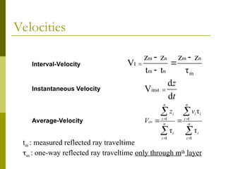
Definitions of velocities (interval, rms, average
etc.)
Dix formula: relation between rms and interval
velocities
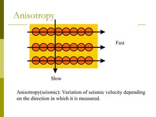
Anisotropy
3.
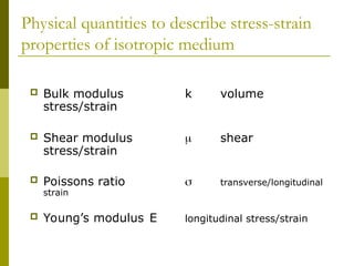
Physical quantities todescribe stress-strain
properties of isotropic medium
Bulk modulus k volume
stress/strain
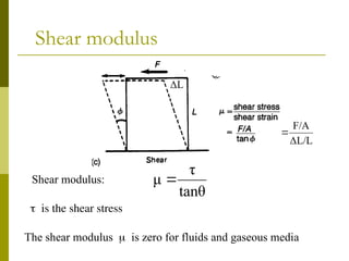
Shear modulus shear
stress/strain
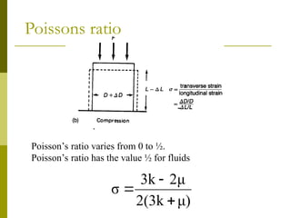
Poissons ratio transverse/longitudinal
strain
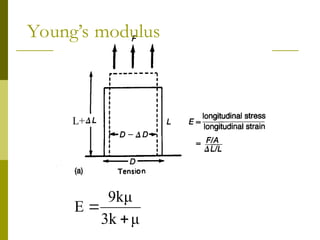
Young’s modulus E longitudinal stress/strain
= Shear modulus
ρ
2μ
λ
ρ
3
4μ
k
p
v
ρ
μ
s
v
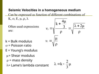
=Lame’s lambda constant μ
3
2
k
λ
Seismic Velocities in a homogeneous medium
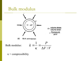
k = Bulk modulus
= mass density
Can be expressed as function of different combinations of
K, , E, , ,
Often used expressions
are:
E = Young’s modulus
= Poisson ratio
9.
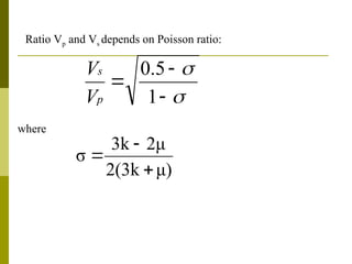
Ratio Vp andVs depends on Poisson ratio:
1
5
.
0
p
s
V
V
μ)
2(3k
2μ
3k
σ
where
10.
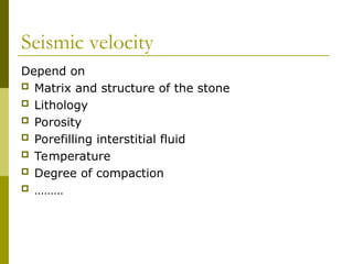
Seismic velocity
Depend on
Matrix and structure of the stone
Lithology
Porosity
Porefilling interstitial fluid
Temperature
Degree of compaction
………
V1, 1
v2 ,2
v3 , 3
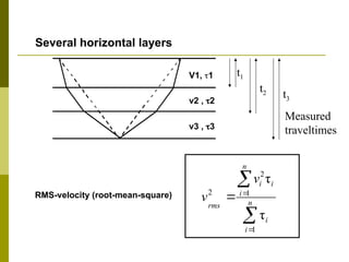
RMS-velocity (root-mean-square)
Several horizontal layers
n
i
i
n
i
i
i
rms
v
v
1
1
2
2
τ
τ
t1
t2 t3
Measured
traveltimes
20.
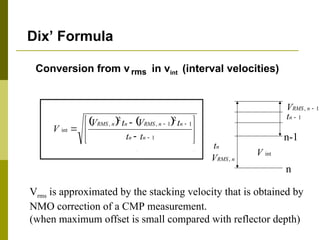
Conversion from vrmsin vint (interval velocities)
Dix’ Formula
n
RMS
V ,
n-1
n
int
V
1
1
2
1
,
2
,
int
n
n
n
n
RMS
n
n
RMS
t
t
t
V
t
V
V
1
,
n
RMS
V
n
t
1
n
t
Vrms is approximated by the stacking velocity that is obtained by
NMO correction of a CMP measurement.
(when maximum offset is small compared with reflector depth)
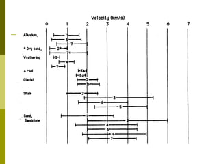
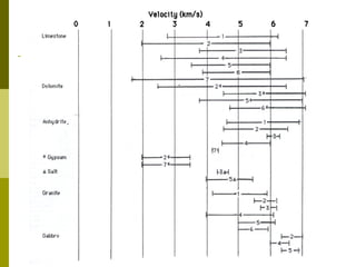
#16 Different people have investigated the velocity of P-waves for various lithologies 1-7. They all found different values
Range of values and the overlap!