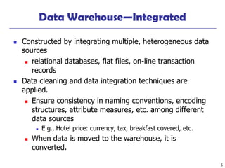
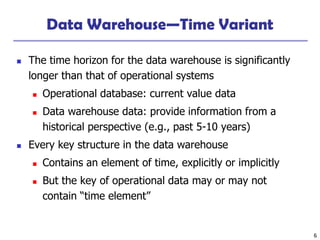
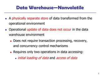
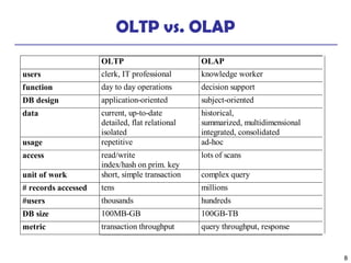
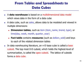
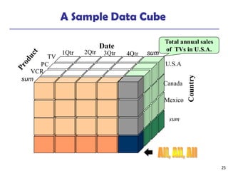
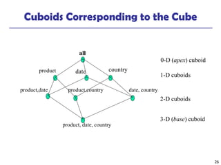
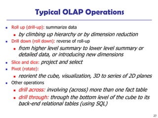
This document discusses data warehousing and online analytical processing (OLAP). It defines a data warehouse as a subject-oriented, integrated, time-variant, and nonvolatile collection of data used for analysis and decision making. The key aspects of a data warehouse covered are its multidimensional data model using cubes and dimensions, extraction of data from multiple sources, and usage for querying, reporting, analytical processing, and data mining. Common data warehouse architectures and operations like star schemas, snowflake schemas, and OLAP functions such as roll-up and drill-down are also summarized.
![39
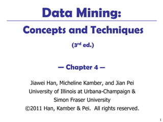
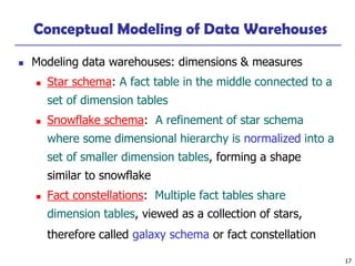
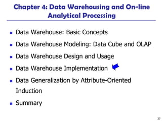
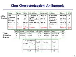
The “Compute Cube” Operator
◼ Cube definition and computation in DMQL
define cube sales [item, city, year]: sum (sales_in_dollars)
compute cube sales
◼ Transform it into a SQL-like language (with a new operator cube
by, introduced by Gray et al.’96)
SELECT item, city, year, SUM (amount)
FROM SALES
CUBE BY item, city, year
◼ Need compute the following Group-Bys
(date, product, customer),
(date,product),(date, customer), (product, customer),
(date), (product), (customer)
()
(item)(city)
()
(year)
(city, item) (city, year) (item, year)
(city, item, year)](https://image.slidesharecdn.com/04olap-191031175733/85/04-olap-39-320.jpg)
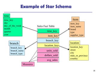
![40
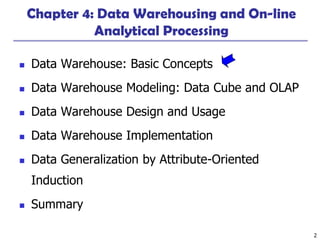
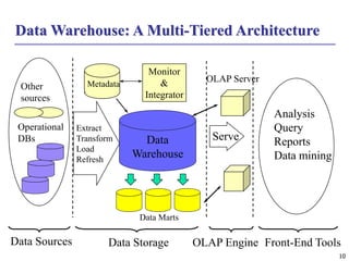
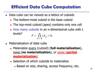
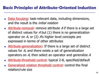
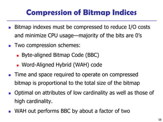
Indexing OLAP Data: Bitmap Index
◼ Index on a particular column
◼ Each value in the column has a bit vector: bit-op is fast
◼ The length of the bit vector: # of records in the base table
◼ The i-th bit is set if the i-th row of the base table has the value for
the indexed column
◼ not suitable for high cardinality domains
◼ A recent bit compression technique, Word-Aligned Hybrid (WAH),
makes it work for high cardinality domain as well [Wu, et al. TODS’06]
Cust Region Type
C1 Asia Retail
C2 Europe Dealer
C3 Asia Dealer
C4 America Retail
C5 Europe Dealer
RecID Retail Dealer
1 1 0
2 0 1
3 0 1
4 1 0
5 0 1
RecIDAsia Europe America
1 1 0 0
2 0 1 0
3 1 0 0
4 0 0 1
5 0 1 0
Base table Index on Region Index on Type](https://image.slidesharecdn.com/04olap-191031175733/85/04-olap-40-320.jpg)
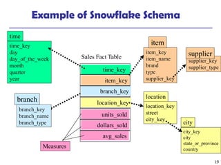
![50
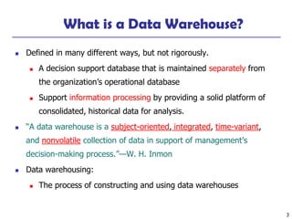
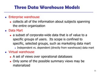
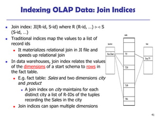
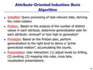
Presentation of Generalized Results
◼ Generalized relation:
◼ Relations where some or all attributes are generalized, with counts
or other aggregation values accumulated.
◼ Cross tabulation:
◼ Mapping results into cross tabulation form (similar to contingency
tables).
◼ Visualization techniques:
◼ Pie charts, bar charts, curves, cubes, and other visual forms.
◼ Quantitative characteristic rules:
◼ Mapping generalized result into characteristic rules with quantitative
information associated with it, e.g.,
.%]47:["")(_%]53:["")(_
)()(
tforeignxregionbirthtCanadaxregionbirth
xmalexgrad
==
](https://image.slidesharecdn.com/04olap-191031175733/85/04-olap-50-320.jpg)


![5G Explained! A High Level Overview [Introduction]](https://cdn.slidesharecdn.com/ss_thumbnails/5gexplainedahighleveloverview-260119165306-cc137a3e-thumbnail.jpg?width=640&height=640&fit=bounds)

