This document proposes a new class of distributions called the Janardan-Power Series (JPS) class by combining the Janardan distribution with the power series family of distributions. It examines the key properties of this class, including the probability density function, survival function, hazard function, moments, quantiles, and order statistics. Some special cases of the JPS distribution are also introduced, such as the Janardan-Binomial, Janardan-Geometric, Janardan-Poisson, and Janardan-Logarithmic distributions. The Janardan-Poisson distribution is analyzed in more detail. Finally, an example is provided applying the JPS distribution to model real data.

1. Journal of Data Science,17(2). P. 259 - 278,2019
DOI:10.6339/JDS.201904_17(2).0002
THE COMPOUND CLASS OF JANARDAN–POWER SERIES
DISTRIBUTIONS: PROPERTIES AND APPLICATIONS
Marzieh Shekari*
, Hossein Zamani*
, Mohammad Mehdi Saber2
*
Department of Statistics, Hormozgan University, Bandar Abbas, Iran.
2
Department of Statistics, College of Sciences, Higher Education Center of Eghlid, Eghlid,
Iran.
Abstract
In the present paper, we propose the new Janardan-Power Series (JPS)
class of distributions, which is a result of combining the Janardan distribution
of Shanker et.al (2013) with the family of power series distributions. Here,
we examine the fundamental attributes of this class of distribution, including
the survival, hazard and reverse hazard functions, limiting behavior of the cdf
and pdf, quantile function, moments and distribution of order statistics.
Moreover, the particular case of the JPS distribution such as the Janardan-
Binomial (JB), Janardan-Geometric (JG), Janardan-Poisson (JP) and the
Janardan-Logarithmic (JL) distributions, are introduced. In addition, the JP
distribution is analyzed in details. Eventually, an example of the proposed
class applied on some real data set.
Keywords: Hazard function, Janardan distribution, Moments, Power series,
order statistics.
*
Corresponding author: Hossein Zamani
Email: zamani.huni@gmail.com

2. 260 THE COMPOUND CLASS OF JANARDAN–POWER SERIES DISTRIBUTIONS:
PROPERTIES AND APPLICATIONS
1. Introduction
Modeling lifetime data is considered in the area of survival analysis, in which the
lifetime of biological organisms or mechanical systems is investigated. Many recently
introduced distributions have the capability to model these types of data appropriately.
The underlying logic and assumptions behind these models is that a lifetime of a system
with 𝑁 (discrete random variable)components and the positive continuous random
variable,𝑋𝑖, which designates the lifetime of the 𝑖𝑡ℎ
component,can be described by a non-
negative random variable 𝑋 = 𝑚𝑖𝑛( 𝑋1, … , 𝑋𝑁) or𝑋 = 𝑚𝑎𝑥( 𝑋1, … , 𝑋𝑁),depending on
whether the components are series or parallel.
Some prominent lifetime distributions are the Exponential Geometric (EG),
Exponential Poisson (EP), Exponential Logarithmic (EL), Weibull Geometric (WG) and
Weibull Poisson (WP), Lindley Logarithmic (LL) distributions, obtained and proposed by
Adamidis and Loukas (1998), Kus (2007), Tahmasbi and Rezaei (2008) ,Barreto-Souza
et al.(2011), Lu and Shi(2011).
The power series class of distributions was examined and derived by Noack (1950),
in which 𝑁 is a discrete random variable depending on the class of power series
distributions with probability mass function
𝑃(𝑁 = 𝑛) =
𝑎𝑛𝜆𝑛
𝐶(𝜆)
, 𝑛 = 1,2, .. (1)
where 𝑎𝑛 ≥ 0 for all 𝑛 = 1,2, … which only relies on n,𝐶( 𝜆) = ∑ 𝑎𝑛𝜆𝑛
∞
𝑛=1 and𝜆 >0, is
fixed in a way that 𝐶( 𝜆) is finite and its first derivative with reference to 𝜆 are determined
and indicated by𝐶′
(. ).
Many novel models have been recently developed by authors utilizing the power series
class of distributions, which some of them have been designed as a combination of some
well-established distributions and the power series class of distributions. For instance;
Exponential-Power Series (EPS) distributions (Ghahkandi and Ganjali, 2009), Weibull-
Power Series (WPS) distributions (Marais and Barreto-Souza,2011), Complementary
Exponential-Power Series (CEPS) distributions (Flores et.al.,2011), Generalized
Exponential-Power Series (GEPS) distributions (Mahmoudi and Jafari,2012), Extended
Weibull-Power Series (EWPS) distributions (Silva et al.,2013), Generalized Extended
Weibull-Power Series (GEWPS) distributions (Alkarni,2016), Kumaraswamy-Power
Series (KPS) distributions (Bidram and Nekoubou,2013), Linear Failure Rate-Power
Series (LFRPS) distributions (Mahmoudi and Jafari,2014) and Lindley-Power series (LPS)
distributions (Warahena-Liyanage and Mavis Pararai, 2015).
Shanker et. al. (2013) proposed a combination of exponential (
𝜃
𝛼
) and gamma (2,
𝜃
𝛼
)
distributions which is known as the Janardan distribution (JD). The Janardan distribution

3. Marzieh Shekari, Hossein Zamani, Mohammad Mehdi Saber 261
is a continuous distribution with two parameters including 𝛼 > 0 𝑎𝑛𝑑 𝜃 > 0 and is
completely characterized by its cumulative distribution function (cdf)
𝐺(𝑥; 𝛼, 𝜃) = 1 − (1 +
𝜃𝛼𝑥
𝜃 + 𝛼2
) 𝑒
−𝜃
𝛼
𝑥
. (2)
for > 0 ,𝛼 > 0 𝑎𝑛𝑑 𝜃 > 0.
For 𝛼 = 1, the distribution reduces to the one parameter Lindley distribution. It has
been proved that the Janardan distribution is a better model compared to the one parameter
Lindley distribution, in terms of analyzing waiting time, survival time and grouped
mortality data.
The rest of this paper is structured as follows. Section 2 introduces the JPS class of
distributions, density, survival, hazard rate and moment generating functions as well as
the moments, quantiles and order statistics .In section 3,the special cases of the JPS
distributions including Janardan-Binomial (JB) distribution, Janardan-Geometric (JG)
distribution, Janardan-Poisson (JP) distribution and Janardan-Logarithmic (JL)
distribution are presented. Furthermore, section 4 examines the Janardan-Poisson (JP)
distribution in greater detail. Section 5 demonstrates an example of the JP distribution
using real data samples. Conclusively, section 6 represents some definitive comments on
the subject.
2. The JPS class of distributions
Suppose that 𝑋1, … , 𝑋𝑁 are independent and identically distributed (iid) random
variables following a Janardan distribution with cdf (2) and N, is a member of the power
series family with the probability mass function given by (1), independent of 𝑋𝑖 .if the
random variable 𝑋 define as 𝑋 = 𝑚𝑖𝑛(𝑋1, … , 𝑋𝑁), then the conditional cdf and pdf of
( X | N n
 ) are respectively defined as:
𝐺( 𝑥; 𝑛) = 1 − 𝑒
−𝑛𝜃
𝛼
𝑥
(1 +
𝜃𝛼𝑥
𝜃 + 𝛼2
)
𝑛
(2)
and
𝑔( 𝑥; 𝑛) =
𝑛𝜃2
𝛼(𝜃 + 𝛼2)
(1 + 𝛼𝑥)𝑒
−𝑛𝜃
𝛼
𝑥
(1 +
𝜃𝛼𝑥
𝜃 + 𝛼2
)
𝑛−1
. (3)
for 𝑥 > 0.
Then the Janardan-Power Series (JPS) class of distributions is given by the marginal
cdf of 𝑋:

4. 262 THE COMPOUND CLASS OF JANARDAN–POWER SERIES DISTRIBUTIONS:
PROPERTIES AND APPLICATIONS
𝐹(𝑥) = 1 −
𝐶 [𝜆𝑒−
𝜃
𝛼
𝑥
(1 +
𝜃𝛼𝑥
𝜃+𝛼2
)]
𝐶(𝜆)
.
(4)
for 𝑥 > 0, 𝛼 > 0, 𝜃 > 0, 𝜆 > 0, in which a random variable 𝑋 denoted by
𝑋~ 𝐽𝑃𝑆(𝛼, 𝜃, 𝜆 ) follows the JPS distribution.
2.1 Density and survival function
The probability density function of a random variable 𝑋 following a JPS distribution
is given by
𝑓(𝑥) =
𝜆𝜃2
𝛼(𝜃 + 𝛼2)
(1 + 𝛼𝑥)𝑒
−𝜃
𝛼
𝑥
𝐶′
[𝜆𝑒−
𝜃
𝛼
𝑥
(1 +
𝜃𝛼𝑥
𝜃+𝛼2
)]
𝐶(𝜆)
; 𝑥 > 0.
(5)
The survival function is given by
𝐹
̄(𝑥) =
𝐶 [𝜆𝑒−
𝜃
𝛼
𝑥
(1 +
𝜃𝛼𝑥
𝜃+𝛼2
)]
𝐶(𝜆)
.
for 𝑥 > 0, 𝛼 > 0, 𝜃 > 0, 𝜆 > 0.
Here some properties of the density (5) are analyzed. The limiting behavior and some
other characteristics of the JPS distribution are studied in the following proposition.
Proposition 2.1. The Janardan distribution is a particular limiting case of the JPS
distribution when𝜆 → 0+
.
Proof. Using𝐶(𝜆) = ∑ 𝑎𝑛𝜆𝑛
∞
𝑛=1 in (4), the following function is obtained:
𝑙𝑖𝑚
𝜆→0+
𝐹(𝑥) = 1 − 𝑙𝑖𝑚
𝜆→0+
𝐶 [𝜆𝑒−
𝜃
𝛼
𝑥
(1 +
𝜃𝛼𝑥
𝜃+𝛼2
)]
𝐶(𝜆)
,
= 1 − 𝑙𝑖𝑚
𝜆→0+
∑ 𝑎𝑛𝜆𝑛
𝑒−
𝑛𝜃
𝛼
𝑥
(1 +
𝜃𝛼𝑥
𝜃+𝛼2
)
𝑛
∞
𝑛=1
∑ 𝑎𝑛𝜆𝑛
∞
𝑛=1
.
and using 𝐿,
𝐻𝑜
̂𝑝𝑖𝑡𝑎𝑙,
𝑠rule, it follows that
𝑙𝑖𝑚
𝜆→0+
𝐹(𝑥) = 1 − 𝑙𝑖𝑚
𝜆→0+
𝑎1 (1 +
𝜃𝛼𝑥
𝜃+𝛼2
) 𝑒
−𝜃𝑥
𝛼 + ∑ 𝑛𝑎𝑛𝜆𝑛−1
(1 +
𝜃𝛼𝑥
𝜃+𝛼2
)
𝑛
𝑒
−𝑛𝜃𝑥
𝛼
∞
𝑛=2
𝑎1 + ∑ 𝑛𝑎𝑛𝜆𝑛−1
∞
𝑛=2
= 1 − (1 +
𝜃𝛼𝑥
𝜃 + 𝛼2
) 𝑒
−𝜃𝑥
𝛼 = 𝐺(𝑥; 𝛼, 𝜃).

5. Marzieh Shekari, Hossein Zamani, Mohammad Mehdi Saber 263
Proposition 2.2. The density function of JPS class can be represented as an infinite linear
combination of the density of minimum order statistic of the i.i.d random variables
following the Janardan distribution.
Proof. By using 𝐶′
(𝜆) = ∑ 𝑛𝑎𝑛𝜆𝑛−1
∞
𝑛=1 in (5), it follows
𝑓(𝑥) = ∑ 𝑃(𝑁 = 𝑛)𝑔(𝑥; 𝑛)
∞
𝑛=1
Where g(x;n) is the pdf of𝑌 = 𝑚𝑖𝑛(𝑋1, … , 𝑋𝑛) given by (3).
Proposition 2.3. For the pdf of the JPS distribution,we have
𝑙𝑖𝑚
𝑥→0+
𝑓(𝑥) =
𝜆𝜃2
𝛼(𝜃 + 𝛼2)
𝐶′
(𝜆)
𝐶(𝜆)
,
and
𝑙𝑖𝑚
𝑥→∞
𝑓(𝑥) = 0.
2.2 Hazard and reversed hazard functions
The hazard and reversed hazard functions of the JPS distributions are respectively
given by
ℎ( 𝑥; 𝛼 , 𝜃, 𝜆) =
𝜆𝜃2
𝛼(𝜃 + 𝛼2)
(1 + 𝛼𝑥)𝑒
−𝜃
𝛼
𝑥
𝐶′
[𝜆 (1 +
𝜃𝛼𝑥
𝜃+𝛼2) 𝑒
−𝜃𝑥
𝛼 ]
𝐶 [𝜆 (1 +
𝜃𝛼𝑥
𝜃+𝛼2
) 𝑒
−𝜃𝑥
𝛼 ]
, (6)
and
𝑟(𝑥; 𝛼 , 𝜃, 𝜆) =
𝜆𝜃2
𝛼(𝜃 + 𝛼2)
(1 + 𝛼𝑥)𝑒
−𝜃
𝛼
𝑥
𝐶′
[𝜆 (1 +
𝜃𝛼𝑥
𝜃+𝛼2
) 𝑒
−𝜃𝑥
𝛼 ]
𝐶(𝜆) − 𝐶 [𝜆 (1 +
𝜃𝛼𝑥
𝜃+𝛼2
) 𝑒
−𝜃𝑥
𝛼 ]
. (7)
where 𝑥 > 0, 𝛼 > 0, 𝜃 > 0 𝑎𝑛𝑑 𝜆 > 0.
2.3 Quantiles, moments and order statistics
The 𝑝𝑡ℎ
quantile of the JPS distributions, for instance 𝑥𝑝, is given by
𝑋𝑝 =
−𝛼
𝜃
−
1
𝛼
−
𝛼
𝜃
𝑊 [
− (1 +
𝜃
𝛼2) 𝐶−1((1 − 𝑝)𝐶(𝜆))
𝜆𝑒
𝜃
𝛼2+1
]. (8)

6. 264 THE COMPOUND CLASS OF JANARDAN–POWER SERIES DISTRIBUTIONS:
PROPERTIES AND APPLICATIONS
for p ∈ (0,1) , 𝐶−1
( . ) is the inverse function of 𝐶(. )and 𝑊( . ) is the negative branch of
the Lambert W function .More details are available at Corless et al. (1996).
Proposition 2.4. The 𝑘𝑡ℎ
moment of JPS distributions is given by
𝐸( 𝑋𝑘
) =
𝜃2
𝐶(𝜆)
∑ 𝑎𝑛𝜆𝑛
𝑛𝛼2𝑛−3
(𝜃 + 𝛼2)𝑛
𝐿1(𝛼, 𝜃, 𝑛, 𝑘)
∞
𝑛=1
(9)
Where
𝐿1(𝛼, 𝜃, 𝑛, 𝑘) = ∑ ∑ (
𝑛 − 1
𝑖
) (
𝑖 + 1
𝑗
)
𝛼2𝑗−2𝑖+𝑘+1
𝛤(𝑗 + 𝑘 + 1)
𝜃𝑗−𝑖+𝑘+1𝑛𝑗+𝑘+1
.
𝑖+1
𝑗=0
𝑛−1
𝑖=0
Proof. We have
𝐸(𝑋𝑘) = ∑ 𝑃(𝑁 = 𝑛)𝐸(𝑌𝑘)
∞
𝑛=1
.
where Y= min(𝑋1, … , 𝑋𝑛) with the pdf of g(x;n).
or ,
𝐸(𝑋𝑘) = ∑ 𝑃(𝑁 = 𝑛) ∫ 𝑥𝑘
𝑔(𝑥; 𝑛)𝑑𝑥
∞
0
∞
𝑛=1
,
= ∑ 𝑃(𝑁 = 𝑛)
𝑛𝛼2𝑛−3
(𝜃 + 𝛼2)𝑛
∫ 𝑥𝑘(1 + 𝛼𝑥) (1 +
𝜃
𝛼2
(1 + 𝛼𝑥))
𝑛−1
𝑒−
𝑛𝜃
𝛼
𝑥
𝑑𝑥
∞
0
∞
𝑛=1
,
= ∑ 𝑃(𝑁 = 𝑛)
𝑛𝛼2𝑛−3
(𝜃 + 𝛼2)𝑛
∞
𝑛=1
𝐿1(𝛼, 𝜃, 𝑛, 𝑘).
where
𝐿1(𝛼, 𝜃, 𝑛, 𝑘) = ∫ 𝑥𝑘(1 + 𝛼𝑥) (1 +
𝜃
𝛼2
(1 + 𝛼𝑥))
𝑛−1
𝑒−
𝑛𝜃
𝛼
𝑥
𝑑𝑥
∞
0
,
= ∫ 𝑥𝑘
𝑒−
𝑛𝜃
𝛼
𝑥
[∑ (
𝑛 − 1
𝑖
) (
𝜃
𝛼2
)
𝑖
(1 + 𝛼𝑥)𝑖+1
𝑛−1
𝑖=0
]
∞
0
𝑑𝑥,
= ∑ ∑ (
𝑛 − 1
𝑖
) (
𝑖 + 1
𝑗
) (
𝜃
𝛼2
)
𝑖
𝛼𝑗
∫ 𝑥𝑗+𝑘
𝑒−
𝑛𝜃
𝛼
𝑥
𝑑𝑥
∞
0
,
𝑖+1
𝑗=0
𝑛−1
𝑖=0

7. Marzieh Shekari, Hossein Zamani, Mohammad Mehdi Saber 265
= ∑ ∑ (
𝑛 − 1
𝑖
) (
𝑖 + 1
𝑗
)
𝛼2𝑗−2𝑖+𝑘+1
𝛤(𝑗 + 𝑘 + 1)
𝜃𝑗−𝑖+𝑘+1𝑛𝑗+𝑘+1
.
𝑖+1
𝑗=0
𝑛−1
𝑖=0
2.4 Order statistics
If 𝑋1, … , 𝑋𝑛 are random variables from a JPS distribution and the 𝑘𝑡ℎ
order statistic is
denoted by𝑋𝑘:𝑛, 𝑘 = 1,2, . . . , 𝑛, then the pdf of 𝑋𝑘:𝑛 is given by
𝑓𝑘:𝑛(𝑥) =
1
𝐵(𝑘, 𝑛 − 𝑘 + 1)
𝑓(𝑥)[𝐹(𝑥)]𝑘−1[1 − 𝐹(𝑥)]𝑛−𝑘
, (8)
Where F(.) and f(.) are the cdf and pdf of JPS distributions respectively given by (4)
and (5), eq. (8) can be written as follows
𝑓𝑘:𝑛(𝑥) =
1
𝐵(𝑘, 𝑛 − 𝑘 + 1)
∑ (
𝑛 − 𝑘
𝑖
) (−1)𝑖
𝑓(𝑥)[𝐹(𝑥)]𝑖+𝑘−1
𝑛−𝑘
𝑖=0
,
In view of the fact that
𝑓(𝑥)[𝐹(𝑥)]𝑖+𝑘−1
=
1
𝑖 + 𝑘
𝑑
𝑑𝑥
[𝐹(𝑥)]𝑖+𝑘
,
The corresponding cdf of 𝑓𝑘:𝑛(𝑥), denoted by 𝐹𝑘:𝑛(𝑥),is given by
𝐹𝑘:𝑛(𝑥) =
1
𝐵(𝑘, 𝑛 − 𝑘 + 1)
∑
(
𝑛 − 𝑘
𝑖
) (−1)𝑖
𝑖 + 𝑘
𝑛−𝑘
𝑖=0
[𝐹(𝑥)]𝑖+𝑘
,
=
1
𝐵(𝑘, 𝑛 − 𝑘 + 1)
∑
(
𝑛 − 𝑘
𝑖
) (−1)𝑖
𝑖 + 𝑘
𝑛−𝑘
𝑖=0
[
1 −
𝐶 (𝜆𝑒−
𝜃
𝛼
𝑥
(1 +
𝜃𝛼𝑥
𝜃+𝛼2
))
𝐶(𝜆)
]
𝑖+𝑘
,
=
1
𝐵(𝑘, 𝑛 − 𝑘 + 1)
∑
(
𝑛 − 𝑘
𝑖
) (−1)𝑖
𝑖 + 𝑘
𝑛−𝑘
𝑖=0
𝐹𝐽(𝑥; 𝛼, 𝜃, 𝜆, 𝑖 + 𝑘)
(9)
Where J is described by an exponential JPS distribution with parameters 𝛼, 𝜃, 𝜆 and
𝑖 + 𝑘.
Thus, the cdf of the 𝑘𝑡ℎ
order statistic can be evaluated as a finite linear combination
of the cdf of the exponential JPS distribution.
Expressions for the moment of the 𝑘𝑡ℎ
order statistics 𝑋𝑘:𝑛, 𝑘 = 1,2, . . . , 𝑛, with cdf
(9), can be obtained using a result of Barakat et al. (2004) as follows:

8. 266 THE COMPOUND CLASS OF JANARDAN–POWER SERIES DISTRIBUTIONS:
PROPERTIES AND APPLICATIONS
𝐸( 𝑋𝑘:𝑛
𝑟
) = ∑ (−1)𝑖−𝑛+𝑘−1
(
𝑖 − 1
𝑛 − 𝑘
) (
𝑛
𝑖
) ∫ 𝑥𝑟−1[𝐹
̄(𝑥)]𝑖
𝑑𝑥
∞
0
𝑛
𝑖=𝑛−𝑘+1
,
= ∑ (−1)𝑖−𝑛+𝑘−1
(
𝑖 − 1
𝑛 − 𝑘
) (
𝑛
𝑖
) ∫ 𝑥𝑟−1
[
𝐶 (𝜆𝑒−
𝜃
𝛼
𝑥
(1 +
𝜃𝛼𝑥
𝜃+𝛼2
))
𝐶(𝜆)
]
𝑖
𝑑𝑥
∞
0
𝑛
𝑖=𝑛−𝑘+1
.
(10)
for 𝑟 = 1,2, . .. and 𝑘 = 1,2, . . . , 𝑛,
An application of the first moment of order statistics can be utilized in calculating the
L-moments, which are in fact the linear combinations of the expected order statistics .For
more details see Hosking (1990).
3. Special cases of the JPS class of distributions
Some particular cases of the class of JPS distribution including the Janardan-Binomial
(JB), Janardan-Geometric (JG), Janardan-Logarithmic (JL) and Janardan-Poisson(JP) are
analyzed in the following section.
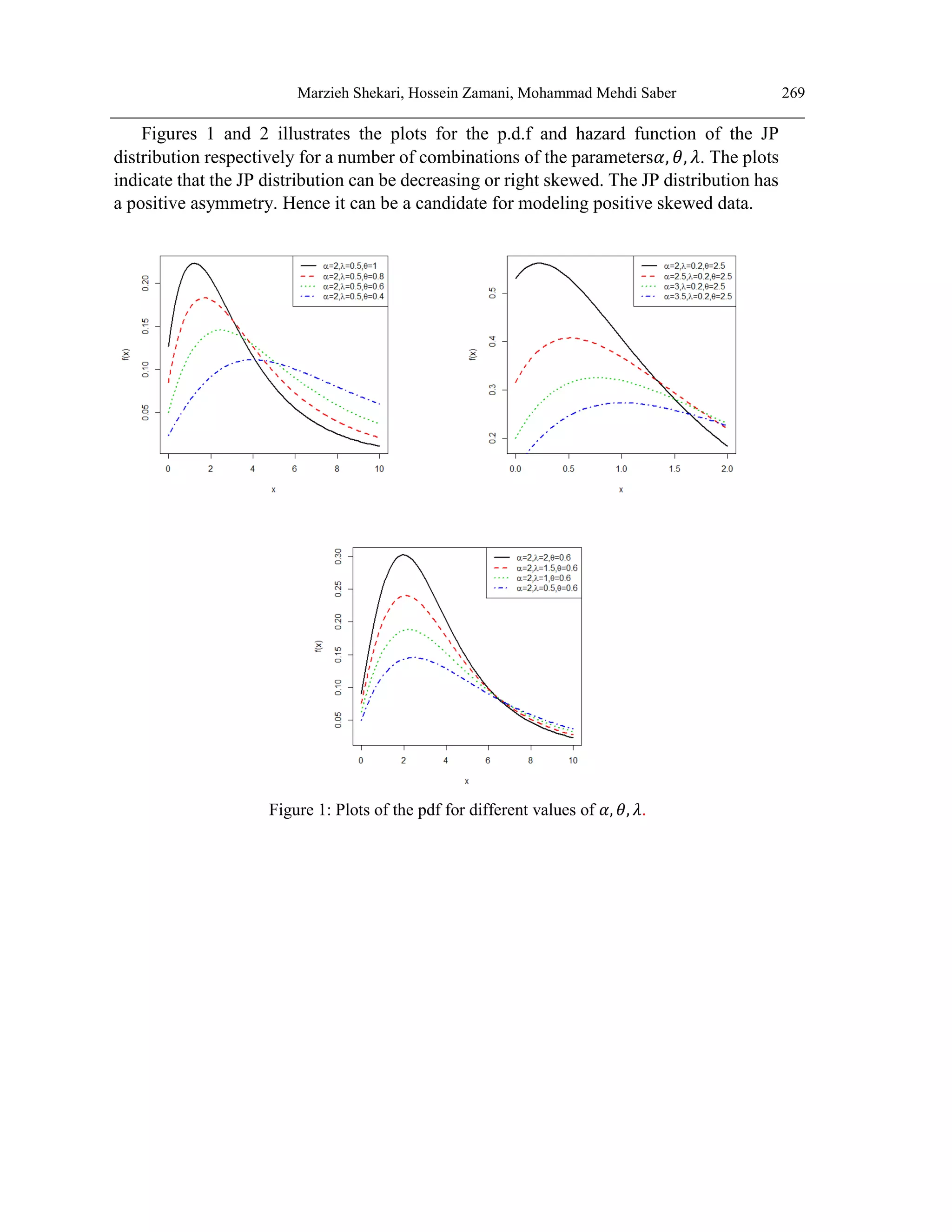
In order to obtain the p.d.f, hazard function and moment, the JP distribution is analyzed.
To determine the flexibility of the JP distribution, plots of the density and hazard rate
functions are presented in Figures 1 and 2 respectively for some selected values of the
parameters.
3.1 Janardan-Binomial distribution
The Janardan-binomial (JB) distribution is determined by the cdf (4) with 𝐶(𝜆) =
(1 + 𝜆)𝑚
− 1, and is given by
𝐹(𝑥) = 1 −
[𝜆𝑒−
𝜃
𝛼
𝑥
(1 +
𝜃𝛼𝑥
𝜃+𝛼2
) + 1]
𝑚
− 1
(1 + 𝜆)𝑚 − 1
.
(11)
Where 𝑥 > 0 , 0 < 𝜆 < 1 and 𝑚is positive integer.
The corresponding p.d.f and hazard rate function are respectively given by
𝑓(𝑥) =
𝑚𝜆𝜃2
𝛼(𝜃 + 𝛼2)
𝑒−
𝜃
𝛼
𝑥
(1 + 𝛼𝑥)
[𝜆𝑒−
𝜃
𝛼
𝑥
(1 +
𝜃𝛼𝑥
𝜃+𝛼2
) + 1]
𝑚−1
(1 + 𝜆)𝑚 − 1
.
(12)
and

9. Marzieh Shekari, Hossein Zamani, Mohammad Mehdi Saber 267
ℎ(𝑥) =
𝑚𝜆𝜃2
𝛼(𝜃 + 𝛼2)
𝑒−
𝜃
𝛼
𝑥
(1 + 𝛼𝑥)
[𝜆𝑒−
𝜃
𝛼
𝑥
(1 +
𝜃𝛼𝑥
𝜃+𝛼2
) + 1]
𝑚−1
[𝜆𝑒−
𝜃
𝛼
𝑥
(1 +
𝜃𝛼𝑥
𝜃+𝛼2
) + 1]
𝑚
− 1
. (13)
Where 𝑥 > 0, 𝛼 > 0, 𝜃 > 0, 𝜆 > 0 and 𝑚 is positive integer.
3.2 Janardan -Geometric distribution
The Janardan-geometric (JG) distribution is characterized by the cdf (4) with 𝐶(𝜆) =
𝜆(1 − 𝜆)−1
,which is given by
𝐹(𝑥) = 1 −
𝑒
−𝜃
𝛼
𝑥
(1 +
𝜃𝛼𝑥
𝜃+𝛼2
) [1 − 𝜆𝑒
−𝜃
𝛼
𝑥
(1 +
𝜃𝛼𝑥
𝜃+𝛼2
)]
−1
(1 − 𝜆)−1
.
𝑥 > 0, 𝛼 > 0, 𝜃 > 0,0 < 𝜆 < 1. (14)
The corresponding pdf and hazard rate function are respectively given by
𝑓(𝑥) =
𝜃2
𝛼(𝜃 + 𝛼2)
𝑒−
𝜃
𝛼
𝑥
(1 + 𝛼𝑥)
(1 − 𝜆)
[1 − 𝜆𝑒−
𝜃
𝛼
𝑥
(1 +
𝜃𝛼𝑥
𝜃+𝛼2
)]
2.
(15)
and
ℎ(𝑥) =
𝜃2
𝛼(𝜃 + 𝛼2)
(1 + 𝛼𝑥)
[1 − 𝜆𝑒−
𝜃
𝛼
𝑥
(1 +
𝜃𝛼𝑥
𝜃+𝛼2
)]
−1
(1 +
𝜃𝛼𝑥
𝜃+𝛼2
)
. (16)
where𝑥 > 0, 𝛼 > 0, 𝜃 > 0,0 < 𝜆 < 1.
3.3 Janardan-Logarithmic distribution
The Janardan-Logarithmic (JL) distribution is characterized by the cdf (4) with
𝐶(𝜆) = − 𝑙𝑜𝑔(1 − 𝜆),which given by
𝐹(𝑥) = 1 −
𝑙𝑜𝑔 [1 − 𝜆 (1 +
𝜃𝛼𝑥
𝜃+𝛼2
) 𝑒
−𝜃
𝛼
𝑥
]
𝑙𝑜𝑔(1 − 𝜆)
.
(17)
for 𝑥 > 0, 𝛼 > 0, 𝜃 > 0,0 < 𝜆 < 1.
The associated p.d.f and hazard rate function are respectively given by
𝑓(𝑥) =
𝜆𝜃2
𝛼(𝜃 + 𝛼2)
(1 + 𝛼𝑥)𝑒
−𝜃
𝛼
𝑥
[1 − 𝜆 (1 +
𝜃𝛼𝑥
𝜃+𝛼2
) 𝑒
−𝜃
𝛼
𝑥
]
−1
− 𝑙𝑜𝑔(1 − 𝜆)
.
(18)
and

10. 268 THE COMPOUND CLASS OF JANARDAN–POWER SERIES DISTRIBUTIONS:
PROPERTIES AND APPLICATIONS
ℎ(𝑥) =
𝜆𝜃2
𝛼(𝜃 + 𝛼2)
(1 + 𝛼𝑥)𝑒
−𝜃
𝛼
𝑥
[1 − 𝜆 (1 +
𝜃𝛼𝑥
𝜃+𝛼2
) 𝑒
−𝜃
𝛼
𝑥
]
−1
− 𝑙𝑜𝑔 [1 − 𝜆 (1 +
𝜃𝛼𝑥
𝜃+𝛼2
) 𝑒
−𝜃
𝛼
𝑥
]
, (19)
for 𝑥 > 0, 𝛼 > 0, 𝜃 > 0,0 < 𝜆 < 1.
4. Janardan-Poisson distribution
This section presents a particular case of JPS class of distributions, the Janardan-
poisson (JP) distribution which will be later explained in detail. The properties of this
distribution are originated from the properties of the general class.
4.1 Survival, density, hazard and reverse hazard functions
The Janardan-Poisson (JP) distribution is characterized by the cdf (4) with 𝐶(𝜆) =
𝑒𝜆
− 1 and 𝑎𝑛 =
1
𝑛!
, where𝜆 > 0.The following equation gives us the survival function of
JP distribution:
𝐹
̄(𝑥) =
𝑒𝑥𝑝 {𝜆 (1 +
𝜃𝛼𝑥
𝜃+𝛼2
) 𝑒
−𝜃
𝛼
𝑥
} − 1
𝑒𝜆 − 1
,
(20)
for 𝑥 > 0, 𝛼 > 0, 𝜃 > 0, 𝜆 > 0.
The corresponding p.d.f, hazard and reverse functions are respectively given by
𝑓(𝑥) =
𝜆𝜃2
𝛼(𝜃 + 𝛼2)
(1 + 𝛼𝑥)𝑒
−𝜃
𝛼
𝑥
𝑒𝑥𝑝 {𝜆 (1 +
𝜃𝛼𝑥
𝜃+𝛼2
) 𝑒
−𝜃
𝛼
𝑥
}
𝑒𝜆 − 1
,
(21)
and
𝒉(𝒙) =
𝝀𝜽𝟐
𝜶(𝜽 + 𝜶𝟐)
(𝟏 + 𝜶𝒙)𝒆
−𝜽
𝜶
𝒙
𝒆𝒙𝒑 {𝝀 (𝟏 +
𝜽𝜶𝒙
𝜽+𝜶𝟐
) 𝒆
−𝜽
𝜶
𝒙
}
𝒆𝒙𝒑 {𝝀 (𝟏 +
𝜽𝜶𝒙
𝜽+𝜶𝟐
)𝒆
−𝜽
𝜶
𝒙
} − 𝟏
, (22)
and
𝒓(𝒙) =
𝝀𝜽𝟐
𝜶(𝜽 + 𝜶𝟐)
(𝟏 + 𝜶𝒙)𝒆
−𝜽
𝜶
𝒙
𝒆𝒙𝒑 {𝝀 (𝟏 +
𝜽𝜶𝒙
𝜽+𝜶𝟐
) 𝒆
−𝜽
𝜶
𝒙
}
𝒆𝝀 − 𝒆𝒙𝒑 {𝝀 (𝟏 +
𝜽𝜶𝒙
𝜽+𝜶𝟐
) 𝒆
−𝜽
𝜶
𝒙
}
, (23)
where 𝑥 > 0, 𝛼 > 0, 𝜃 > 0, 𝜆 > 0.

11. Marzieh Shekari, Hossein Zamani, Mohammad Mehdi Saber 269
Figures 1 and 2 illustrates the plots for the p.d.f and hazard function of the JP
distribution respectively for a number of combinations of the parameters𝛼, 𝜃, 𝜆. The plots
indicate that the JP distribution can be decreasing or right skewed. The JP distribution has
a positive asymmetry. Hence it can be a candidate for modeling positive skewed data.
Figure 1: Plots of the pdf for different values of 𝛼, 𝜃, 𝜆.

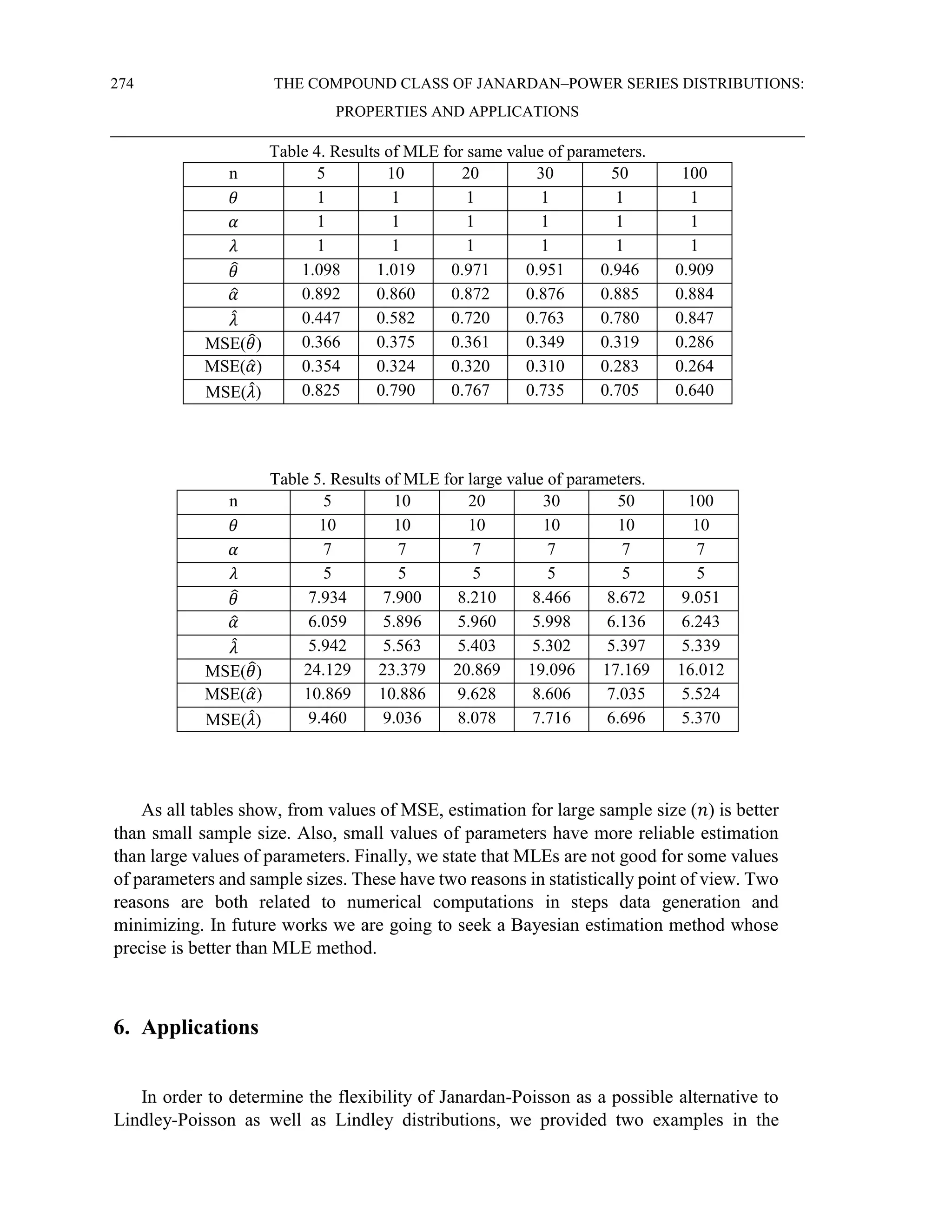
12. 270 THE COMPOUND CLASS OF JANARDAN–POWER SERIES DISTRIBUTIONS:
PROPERTIES AND APPLICATIONS
Figure 2: Plots of the hazard rate function for different value of 𝛼, 𝜃, 𝜆.
The plots for the hazard function of JP distribution exhibit different shapes including
monotonically increasing, increasing-decreasing and increasing-decreasing-increasing
shapes. These interesting shapes of the hazard function indicate that JP distribution is
suitable for monotonic and non-monotonic hazard behaviors which are more likely to be
encountered in real life situations.
4.2 Quantiles and median
By substituting 𝐶−1(𝜆) = 𝑙𝑜𝑔(1 + 𝜆) in equation (6), the quantiles and median for
the JP distribution are respectively given as
𝑋𝑝 =
−𝛼
𝜃
−
1
𝛼
−
𝛼
𝜃
𝑊 [
− (1 +
𝜃
𝛼2
) 𝑙𝑜𝑔 (1 + (1 − 𝑝)(𝑒𝜆
− 1))
𝜆𝑒
𝜃
𝛼2+1
] , 0 < 𝑝 < 1, (24)
and

13. Marzieh Shekari, Hossein Zamani, Mohammad Mehdi Saber 271
𝑚 =
−𝛼
𝜃
−
1
𝛼
−
𝛼
𝜃
𝑊 [
− (1 +
𝜃
𝛼2
) 𝑙𝑜𝑔 (1 +
1
2
(𝑒𝜆
− 1))
𝜆𝑒
𝜃
𝛼2+1
], (25)
with 𝑊(. )as the negative branch of the Lambert 𝑊 function.
4.3 Moments and moment generating function
The 𝑘𝑡ℎ
moment of a random variable 𝑋 from the JP distribution is given by
𝐸(𝑋𝑘) = ∑
𝜆𝑛
𝜃2
𝛼2𝑛−3
𝐿1(𝛼, 𝜃, 𝑛, 𝑘)
(𝑛 − 1)! (𝑒𝜆 − 1)(𝜃 + 𝛼2)𝑛
∞
𝑛=1
(26)
The first six moments , standard deviation (SD), coefficient of variation (CV),
coefficient of skewness (CS) and coefficient of kurtosis (CK) of the JP distribution for
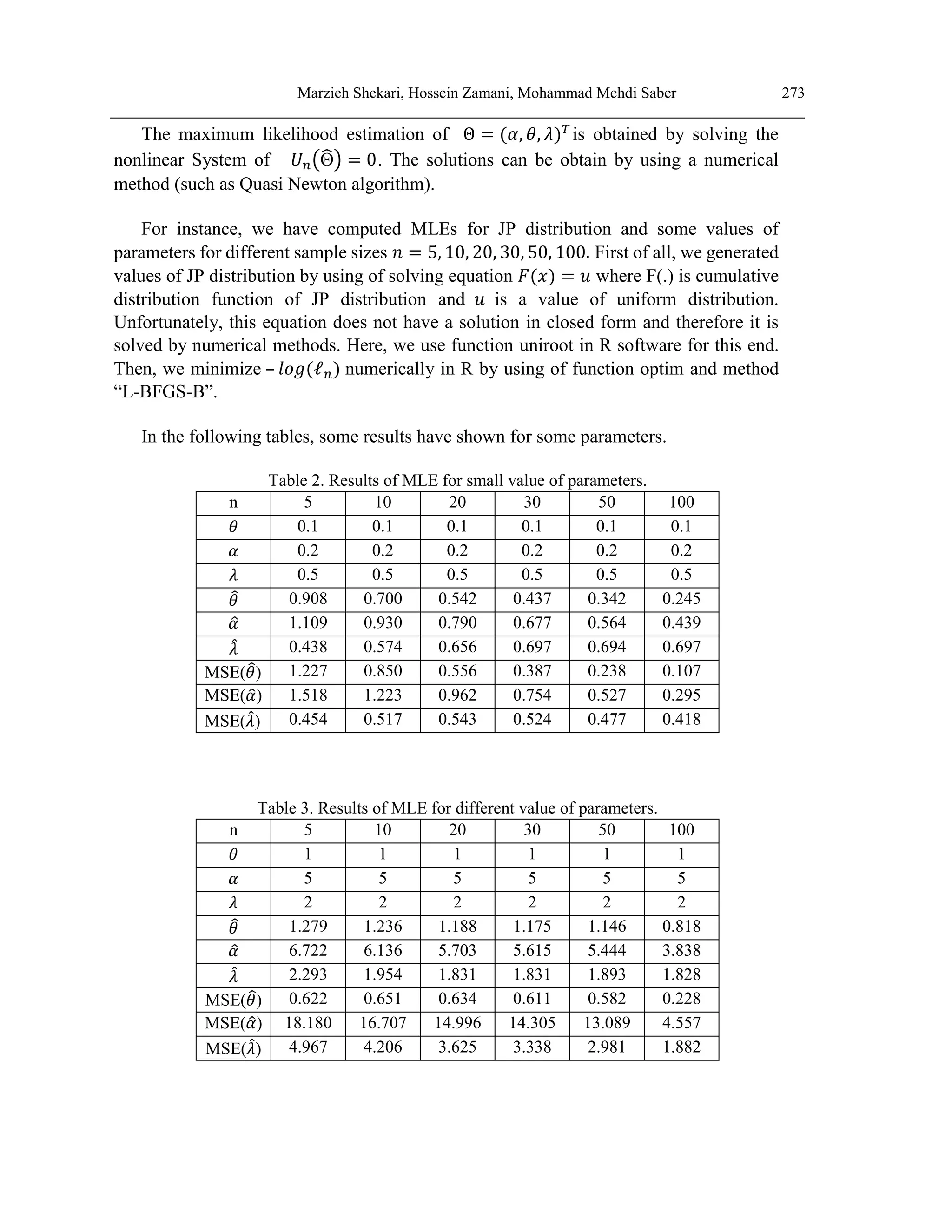
some selected values of the parameters 𝛼, 𝜃, 𝜆 are provided in table 1.
Table 1: Moments of JP distribution for some values of 𝛼, 𝜃, 𝜆.
𝜇𝑘
′
𝛽
̂ = 1.5, 𝜆
̂ = 0.2,
𝛼
̂ = 1
𝛽
̂ = 1.5, 𝜆
̂ = 0.2,
𝛼
̂ = 1.5
𝛽
̂ = 2.5, 𝜆
̂ = 0.8,
𝛼
̂ = 1.5
𝛽
̂ = 2.5, 𝜆
̂ = 0.8,
𝛼
̂ = 2.5
𝜇1
′ 0.8897 1.5296 0.7283 1.4347
𝜇2
′ 1.4876 4.1027 1.0380 3.6542
𝜇3
′ 3.5880 15.4453 2.1921 13.3277
𝜇4
′ 11.2268 74.4287 6.0953 63.1371
SD 0.8342 1.3277 0.7124 1.2632
CV 0.9376 0.8680 0.9781 0.8804
CS 1.7672 1.6134 1.9269 1.7393
CK 7.5231 6.7901 8.4194 7.4902
The moment generating function (mgf) of the JP distribution is given by
𝑀(𝑡) = ∑
𝑡𝑘
𝑘!
∞
𝑘=0
𝐸(𝑋𝑘)
= ∑ ∑
𝑡𝑘
𝑘!
∞
𝑘=0
∞
𝑛=1
𝜆𝑛
𝜃2
𝛼2𝑛−3
𝐿1(𝛼, 𝜃, 𝑛, 𝑘)
(𝑛 − 1)! (𝑒𝜆 − 1)(𝜃 + 𝛼2)𝑛
.
(27)
4.4 Cdf and p.d.f of order statistics
By using the cdf of the JP distribution as an alternative to (9), the cdf and p.d.f of the
𝑘𝑡ℎ
order statistics respectively provided as
𝐹𝑘:𝑛(𝑥) =
1
𝐵(𝑘, 𝑛 − 𝑘 + 1)
∑ (−1)𝑖
(
𝑛 − 𝑘
𝑖
)
𝑛−𝑘
𝑖=0
𝑖 + 𝑘
(1 −
𝑒𝑥𝑝 {𝜆 (1 +
𝜃𝛼𝑥
𝜃+𝛼2) 𝑒
−𝜃
𝛼
𝑥
} − 1
𝑒𝜆 − 1
)
𝑖+𝑘
, (28)

14. 272 THE COMPOUND CLASS OF JANARDAN–POWER SERIES DISTRIBUTIONS:
PROPERTIES AND APPLICATIONS
and
𝑓𝑘:𝑛(𝑥) =
1
𝐵(𝑘,𝑛−𝑘+1)
∑ (−1)𝑖(
𝑛−𝑘
𝑖
)
𝑛−𝑘
𝑖=0
𝑖+𝑘
𝜆𝜃2
𝛼(𝜃+𝛼2)
(1 + 𝛼𝑥)𝑒
−𝜃
𝛼
𝑥
𝑒𝑥𝑝{𝜆(1+
𝜃𝛼𝑥
𝜃+𝛼2)𝑒
−𝜃
𝛼
𝑥
}
(𝑒𝜆−1)𝑖+𝑘
× (𝑒𝜆
− 𝑒𝑥𝑝 {𝜆 (1 +
𝜃𝛼𝑥
𝜃+𝛼2) 𝑒
−𝜃
𝛼
𝑥
})
𝑖+𝑘−1
, (29)
Where 𝑥 > 0, 𝛼 > 0, 𝜃 > 0, 𝜆 > 0.
5. Maximum Likelihood Estimation
Let 𝑥1, . . . , 𝑥𝑛be the observations of a random sample of size 𝑛 from the 𝐽𝑃𝑆(𝛼, 𝜃, 𝜆)
distributions. The log-likelihood function for the vector of Θ = (𝛼, 𝜃, 𝜆)𝑇
is given by
ℓ𝑛 = ℓ𝑛(𝛩, 𝑥1, … , 𝑥𝑛) = 𝑛 𝑙𝑜𝑔( 𝜆) + 2𝑛 𝑙𝑜𝑔( 𝜃) − 𝑛 𝑙𝑜𝑔( 𝛼)
−𝑛 𝑙𝑜𝑔( 𝜃 + 𝛼2
) + ∑ 𝑙𝑛 𝐶′ (𝜆𝑝𝑖)
𝑛
𝑖=1
− 𝑛 𝑙𝑛 𝐶 (𝜆)
+ ∑ 𝑙𝑛(1 + 𝛼𝑥𝑖)
𝑛
𝑖=1
−
𝜃
𝛼
∑ 𝑥𝑖
𝑛
𝑖=1 (30)
where 𝑝𝑖 = 𝑒
−𝜃
𝛼
𝑥𝑖
(1 +
𝜃𝛼𝑥𝑖
𝜃+𝛼2
).
The score vector is given by 𝑈𝑛(Θ) = (
∂ℓ𝑛
∂𝛼
,
∂ℓ𝑛
∂𝜃
,
∂ℓ𝑛
∂𝜆
)
𝑇
with the components
𝜕ℓ𝑛
𝜕𝛼
=
−𝑛
𝛼
−
2𝑛𝛼
𝜃 + 𝛼2
+ ∑
(𝜆𝑝𝑖 (
𝜃𝑥𝑖
𝛼2
+
𝜃𝑥𝑖(𝜃−𝛼2)
(𝜃+𝛼2+𝜃𝛼𝑥𝑖)(𝜃+𝛼2)
) ) 𝐶″(𝜆𝑝𝑖)
𝐶′(𝜆𝑝𝑖)
𝑛
𝑖=1
+ ∑
𝑥𝑖
1 + 𝛼𝑥𝑖
+
𝑛
𝑖=1
𝜃
𝛼2
∑ 𝑥𝑖
𝑛
𝑖=1
.
𝜕ℓ𝑛
𝜕𝜃
=
2𝑛
𝜃
−
𝑛
𝜃 + 𝛼2
+ ∑
(𝜆𝑝𝑖 (
𝛼3𝑥𝑖
(𝜃+𝛼2+𝜃𝛼𝑥𝑖)(𝜃+𝛼2)
−
𝑥𝑖
𝛼
)) 𝐶″(𝜆𝑝𝑖)
𝐶′(𝜆𝑝𝑖)
𝑛
𝑖=1
−
1
𝛼
∑ 𝑥𝑖
𝑛
𝑖=1
,
𝜕ℓ𝑛
𝜕𝜆
=
𝑛
𝜆
+ ∑
𝑝𝑖𝐶″(𝜆𝑝𝑖)
𝐶′(𝜆𝑝𝑖)
𝑛
𝑖=1
−
𝑛𝐶′(𝜆)
𝐶(𝜆)
.

15. Marzieh Shekari, Hossein Zamani, Mohammad Mehdi Saber 273
The maximum likelihood estimation of Θ = (𝛼, 𝜃, 𝜆)𝑇
is obtained by solving the
nonlinear System of 𝑈𝑛(Θ
̂) = 0. The solutions can be obtain by using a numerical
method (such as Quasi Newton algorithm).
For instance, we have computed MLEs for JP distribution and some values of
parameters for different sample sizes 𝑛 = 5, 10, 20, 30, 50, 100. First of all, we generated
values of JP distribution by using of solving equation 𝐹(𝑥) = 𝑢 where F(.) is cumulative
distribution function of JP distribution and 𝑢 is a value of uniform distribution.
Unfortunately, this equation does not have a solution in closed form and therefore it is
solved by numerical methods. Here, we use function uniroot in R software for this end.
Then, we minimize – 𝑙𝑜𝑔(ℓ𝑛) numerically in R by using of function optim and method
“L-BFGS-B”.
In the following tables, some results have shown for some parameters.
Table 2. Results of MLE for small value of parameters.
n 5 10 20 30 50 100
𝜃 0.1 0.1 0.1 0.1 0.1 0.1
𝛼 0.2 0.2 0.2 0.2 0.2 0.2
𝜆 0.5 0.5 0.5 0.5 0.5 0.5
𝜃
̂ 0.908 0.700 0.542 0.437 0.342 0.245
𝛼
̂ 1.109 0.930 0.790 0.677 0.564 0.439
𝜆
̂ 0.438 0.574 0.656 0.697 0.694 0.697
MSE(𝜃
̂) 1.227 0.850 0.556 0.387 0.238 0.107
MSE(𝛼
̂) 1.518 1.223 0.962 0.754 0.527 0.295
MSE(𝜆
̂) 0.454 0.517 0.543 0.524 0.477 0.418
Table 3. Results of MLE for different value of parameters.
n 5 10 20 30 50 100
𝜃 1 1 1 1 1 1
𝛼 5 5 5 5 5 5
𝜆 2 2 2 2 2 2
𝜃
̂ 1.279 1.236 1.188 1.175 1.146 0.818
𝛼
̂ 6.722 6.136 5.703 5.615 5.444 3.838
𝜆
̂ 2.293 1.954 1.831 1.831 1.893 1.828
MSE(𝜃
̂) 0.622 0.651 0.634 0.611 0.582 0.228
MSE(𝛼
̂) 18.180 16.707 14.996 14.305 13.089 4.557
MSE(𝜆
̂) 4.967 4.206 3.625 3.338 2.981 1.882

16. 274 THE COMPOUND CLASS OF JANARDAN–POWER SERIES DISTRIBUTIONS:
PROPERTIES AND APPLICATIONS
Table 4. Results of MLE for same value of parameters.
n 5 10 20 30 50 100
𝜃 1 1 1 1 1 1
𝛼 1 1 1 1 1 1
𝜆 1 1 1 1 1 1
𝜃
̂ 1.098 1.019 0.971 0.951 0.946 0.909
𝛼
̂ 0.892 0.860 0.872 0.876 0.885 0.884
𝜆
̂ 0.447 0.582 0.720 0.763 0.780 0.847
MSE(𝜃
̂) 0.366 0.375 0.361 0.349 0.319 0.286
MSE(𝛼
̂) 0.354 0.324 0.320 0.310 0.283 0.264
MSE(𝜆
̂) 0.825 0.790 0.767 0.735 0.705 0.640
Table 5. Results of MLE for large value of parameters.
n 5 10 20 30 50 100
𝜃 10 10 10 10 10 10
𝛼 7 7 7 7 7 7
𝜆 5 5 5 5 5 5
𝜃
̂ 7.934 7.900 8.210 8.466 8.672 9.051
𝛼
̂ 6.059 5.896 5.960 5.998 6.136 6.243
𝜆
̂ 5.942 5.563 5.403 5.302 5.397 5.339
MSE(𝜃
̂) 24.129 23.379 20.869 19.096 17.169 16.012
MSE(𝛼
̂) 10.869 10.886 9.628 8.606 7.035 5.524
MSE(𝜆
̂) 9.460 9.036 8.078 7.716 6.696 5.370
As all tables show, from values of MSE, estimation for large sample size (𝑛) is better
than small sample size. Also, small values of parameters have more reliable estimation
than large values of parameters. Finally, we state that MLEs are not good for some values
of parameters and sample sizes. These have two reasons in statistically point of view. Two
reasons are both related to numerical computations in steps data generation and
minimizing. In future works we are going to seek a Bayesian estimation method whose
precise is better than MLE method.
6. Applications
In order to determine the flexibility of Janardan-Poisson as a possible alternative to
Lindley-Poisson as well as Lindley distributions, we provided two examples in the

17. Marzieh Shekari, Hossein Zamani, Mohammad Mehdi Saber 275
following section. For both examples, the data histogram, probabilities and the plots of
fitted densities are presented with real data.
Example 1:
The waiting times (in minutes) to receive banking services for 100 customers are
provided in the first data set by Ghitany et al.(2008). Estimates of parameters of JP, LP
and Lindley distributions with AIC are provided in Table 6.
Table 6: Estimates of models for waiting data.
Distributions 𝛽 𝜆 𝛼 -2log L
Lindley 0.187 - - 643.39
Lindley-Poisson 0.057 7.367 - 642.3
Janardan-Poisson 3.717 0.526 20.3 639.79
The AIC of the fitted models indicates that the JP leads to a better fitting to data
compared to LP and Lindley distributions. The plots of fitted densities and histogram of
data are given in Figure3.
Figure 3: Histogram and fitted density plots for waiting data.
Example 2:
This data set represents the lifetime’s data relating to relief times (in minutes) of 20
patients receiving an analgesic which reported by Gross et al. (1975) and applied by
Shankar et.al (2016).

18. 276 THE COMPOUND CLASS OF JANARDAN–POWER SERIES DISTRIBUTIONS:
PROPERTIES AND APPLICATIONS
Figure 4 illustrates the fitted densities plot as well as the data histogram.
Figure 4: Histogram and fitted density plots for life time data.
Table 7 represents the results of the AIC along with the parameters of JP, LP and
Lindley distributions.
Table 7: Estimates of models for life time data.
Distributions 𝛽 𝜆 𝛼 -2log L
Lindley 0.8161 - - 62.48
Lindley-Poisson 0.0192 709.76 - 57.6
Janardan-Poisson 4.125 694.7 152.66 51.32
The AIC of the fitted models revealed that the JP is markedly better fitted to the dataset
in comparison to LP and Lindley distributions.

19. Marzieh Shekari, Hossein Zamani, Mohammad Mehdi Saber 277
References
[1] Alkarni, S. H. (2016). Generalized extended Weibull power series family of distributions.
Journal of Data Science, 14, 415-440.
[2] Barreto-Souza, W., Morais, A. L. and Cordeiro, G. M. (2011). The Weibull-geometric
distribution. Journal of Statistical Computation and Simulation, 81, 645-657.
[3] Bidram, H. and Nekoukhou, V. (2013). Double bounded Kumaraswamy-power series class
of distributions. SORT-Statistics and Operations Research Transactions, 1(2), 211-230.
[4] Corless, R .M., Gounet, G.H., Hare, D. E., Jeffrey, D. J. and Knuth, D. E. (1996). On the
lambert W function. Advances in Computational Mathematics, 5(1), 329-359.
[5] Chahkandi, M. and Ganjali, M. (2009). On some lifetime distributions with decreasing
failure rate. Computational Statistics and Data Analysis, 53, 4433-4440.
[6] Flores, J. D., Borges, P., Cancho, V. G. and Louzada, F. (2013). The complementary
exponential power series distributions. Brazilian Journal of Probability and Statistics, 4, 565-
585.
[7] Ghitany, M. E., Atieh, B., & Nadarajah, S. (2008). Lindley distribution and its application.
Mathematics and computers in simulation, 78(4), 493-506.
[8] Gross AJ, Clark VA (1975) Survival Distributions Reliability Applications in the Biometrical
Sciences. John Wiley, New York, USA.
[9] Hosking, J. R. M. (1990). L-moments: Analysis and estimation of distributions using linear
combinations of order statistics. Journal of the Royal Statistical Society, Series B, 52, 105-
124.
[10] Johnson, N. L., Kemp, A. W. and Kotz, S. (2005). Univariate discrete distributions. John
Wiley & sons.
[11] Kus, C. (2007). A new lifetime distribution. Computational Statistics and Data Analysis,
51(9), 4496-4509.
[12] Lu, W. and Shi, D. (2012). A new compounding life distribution: The Weibull Poisson
distribution. Journal of Applied Statistics, 39(1), 21-38.
[13] Mahmoudi, E. and Jafari, A. A. (2012). Generalized exponential–power series distributions.
Computational Statistics and Data Analysis, 56, 4047-4066.
[14] Mahmoudi, E. and Jafari, A.A. (2014). The Compound Class of Linear Failure Rate–Power
Series distributions: Model, Properties and Applications. arXiv preprint arXiv:1402.5282.
[15] Morais, A. L. and Barreto–Souza, W. (2011). A compound class of Weibull and power series
distributions. Computational Statistics and Data Analysis, 55, 1410-1425.
[16] Noack, A. (1950). A class of random variables with discrete distributions. Annals of
Mathematical Statistics, 1,127-132.

20. 278 THE COMPOUND CLASS OF JANARDAN–POWER SERIES DISTRIBUTIONS:
PROPERTIES AND APPLICATIONS
[17] Shanker, R. Fresshaye, H. and Sharma, S. (2016). On Two-Parameter Lindley Distribution
and its Applications to Model Liftime Data. Biometrics & Biostatistics International Journal,
1(3),1-8.
[18] Shanker, R., Sharma, S., Shanker, U. and Shanker, R. (2013). Janardan distribution and its
application to waiting Times Data. Indian Journal of Applied Research, 3(8), ISSN-2249-
555X
[19] Silva, R. B., Bourguignon, M., Dias, C. R. B. and Cordeiro, G. M. (2013). The compound
class of extended Weibull power series distributions. Computational Statistics and Data
Analysis, 58, 352-367.
[20] Tahmasbi, R. and Rezaei, S. (2008). A two- parameter lifetime distribution with decreasing
failure rate. Computational Statistics and Data Analysis, 52, 3889-3901.
[21] Warahena- Liyanage, G. and Pararai, M. (2015). The Lindley Power Series Class of
Distributions. Model, Properties and Applications. Journal of Computations & Modeling,
5(3), 35-80.