Problem 9-17 1. Collections on sales: July August Sept. Quarter Cash sales $ 8,000 $14,000 $10,000 $ 32,000 Credit sales: May: $30,000 × 80% × 20% 4,800 4,800 June: $36,000 × 80% × 70%, 20% 20,160 5,760 25,920 July: $40,000 × 80% × 10%, 70%, 20% 3,200 22,400 6,400 32,000 Aug.: $70,000 × 80% × 10%, 70% 5,600 39,200 44,800 Sept.: $50,000 × 80% × 10%    4,000      4,000 Total cash collections $36,160 $47,760 $59,600 $143,520 2. a. Merchandise purchases budget: July August Sept. Oct. Budgeted cost of goods sold $24,000 $42,000 $30,000 $27,000 Add desired ending inventory*  31,500  22,500  20,250 Total needs 55,500 64,500 50,250 Less beginning inventory  18,000  31,500  22,500 Required inventory purchases $37,500 $33,000 $27,750 *75% of the next month’s budgeted cost of goods sold. b. Schedule of expected cash disbursements for merchandise purchases: July August Sept. Quarter Accounts payable, June 30 $11,700 $11,700 July purchases 18,750 $18,750 37,500 August purchases 16,500 $16,500 33,000 September purchases  13,875  13,875 Total cash disbursements $30,450 $35,250 $30,375 $96,075 3. Janus Products, Inc. Cash Budget For the Quarter Ended September 30 July August Sept. Quarter Cash balance, beginning $ 8,000 $ 8,410 $ 8,020 $   8,000 Add collections from sales  36,160  47,760  59,600  143,520 Total cash available  44,160  56,170  67,620  151,520 Less disbursements: For inventory purchases 30,450 35,250 30,375 96,075 For selling expenses 7,200 11,700 8,500 27,400 For administrative expenses 3,600 5,200 4,100 12,900 For land 4,500 0 0 4,500 For dividends         0          0    1,000     1,000 Total disbursements  45,750  52,150  43,975  141,875 Excess (deficiency) of cash available over disbursements  (1,590)    4,020  23,645     9,645 Financing: Borrowings 10,000 4,000 14,000 Repayment 0 0 (14,000) (14,000) Interest          0          0     (380)       (380) Total financing  10,000    4,000 (14,380)       (380) Cash balance, ending $ 8,410 $ 8,020 $ 9,265 $   9,265 * $10,000 × 1% × 3 = $300 $4,000 × 1% × 2 =    80 $380 Problem 9-19 1. The sales budget for the third quarter: July Aug. Sept. Quarter Budgeted sales (pairs) 6,000 7,000 8,000 18,000 Selling price per pair × $50 × $50 × $50 × $50 Total budgeted sales $300,000 $350,000 $400,000 $900,000 The schedule of expected cash collections from sales: July Aug. Sept. Quarter Accounts receivable, beginning balance $130,000 $130,000 July sales: $300,000 × 40%, 50% 120,000 $150,000 270,000 August sales: $350,000 × 40%, 50% 140,000 $175,000 315,000 September sales: $400,000 × 40%  160,000  160,000 Total cash collections $250,000 $290,000 $335,000 $875,000 2. The production budget for July through October: July Aug. Sept. Oct. Budgeted sales (pairs) 6,000 7,000 8,000 4,000 Add desired ending inventory    700   800   400   300 Total needs 6,700 7,80.

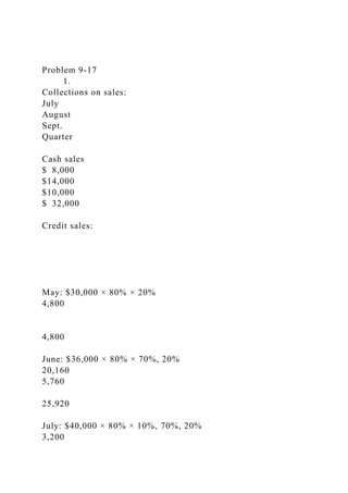
1. Problem 9-17
1.
Collections on sales:
July
August
Sept.
Quarter
Cash sales
$ 8,000
$14,000
$10,000
$ 32,000
Credit sales:
May: $30,000 × 80% × 20%
4,800
4,800
June: $36,000 × 80% × 70%, 20%
20,160
5,760
25,920
July: $40,000 × 80% × 10%, 70%, 20%
3,200

2. 22,400
6,400
32,000
Aug.: $70,000 × 80% × 10%, 70%
5,600
39,200
44,800
Sept.: $50,000 × 80% × 10%
4,000
4,000
Total cash collections
$36,160
$47,760
$59,600
$143,520
2. a. Merchandise purchases budget:
July
August
Sept.
Oct.
Budgeted cost of goods sold
$24,000
$42,000
$30,000
$27,000
Add desired ending inventory*
31,500

3. 22,500
20,250
Total needs
55,500
64,500
50,250
Less beginning inventory
18,000
31,500
22,500
Required inventory purchases
$37,500
$33,000
$27,750
*75% of the next month’s budgeted cost of
goods sold.
b. Schedule of expected cash disbursements for
merchandise purchases:
July
August
Sept.
Quarter
Accounts payable, June 30
$11,700
$11,700
July purchases

4. 18,750
$18,750
37,500
August purchases
16,500
$16,500
33,000
September purchases
13,875
13,875
Total cash disbursements
$30,450
$35,250
$30,375
$96,075
3.
Janus Products, Inc.
Cash Budget
For the Quarter Ended September 30
July
August
Sept.
Quarter
Cash balance, beginning
$ 8,000
$ 8,410
$ 8,020

5. $ 8,000
Add collections from sales
36,160
47,760
59,600
143,520
Total cash available
44,160
56,170
67,620
151,520
Less disbursements:
For inventory purchases
30,450
35,250
30,375
96,075
For selling expenses
7,200
11,700
8,500
27,400
For administrative expenses
3,600
5,200
4,100

6. 12,900
For land
4,500
0
0
4,500
For dividends
0
0
1,000
1,000
Total disbursements
45,750
52,150
43,975
141,875
Excess (deficiency) of cash available over disbursements
(1,590)
4,020
23,645
9,645
Financing:
Borrowings
10,000
4,000

7. 14,000
Repayment
0
0
(14,000)
(14,000)
Interest
0
0
(380)
(380)
Total financing
10,000
4,000
(14,380)
(380)
Cash balance, ending
$ 8,410
$ 8,020
$ 9,265
$ 9,265
*
$10,000 × 1% × 3 =
$300
$4,000 × 1% × 2 =
80
$380

8. Problem 9-19
1. The sales budget for the third quarter:
July
Aug.
Sept.
Quarter
Budgeted sales (pairs)
6,000
7,000
8,000
18,000
Selling price per pair
× $50
× $50
× $50
× $50
Total budgeted sales
$300,000
$350,000
$400,000
$900,000
The schedule of expected cash collections from sales:
July
Aug.
Sept.
Quarter
Accounts receivable, beginning balance
$130,000
$130,000

9. July sales:
$300,000 × 40%, 50%
120,000
$150,000
270,000
August sales:
$350,000 × 40%, 50%
140,000
$175,000
315,000
September sales:
$400,000 × 40%
160,000
160,000
Total cash collections
$250,000
$290,000
$335,000
$875,000
2. The production budget for July through October:
July
Aug.
Sept.
Oct.
Budgeted sales (pairs)
6,000
7,000
8,000
4,000

10. Add desired ending inventory
700
800
400
300
Total needs
6,700
7,800
8,400
4,300
Less beginning inventory
600
700
800
400
Required production (pairs)
6,100
7,100
7,600
3,900
3. The direct materials budget for the third quarter:
July
Aug.
Sept.
Quarter
Required production—pairs (above)
6,100
7,100
7,600

11. 20,800
Raw materials needs per pair
× 2lbs.
× 2lbs.
× 2lbs.
× 2lbs.
Production needs (lbs.)
12,200
14,200
15,200
41,600
Add desired ending inventory
2,840
3,040
1,560
*
1,560
Total needs
15,040
17,240
16,760
49,040
Less beginning inventory
2,440

12. 2,840
3,040
2,440
Raw materials to be purchased
12,600
14,400
13720
40,720
Cost of raw materials to be purchased at $2.50 per lb.
$31,500
$36,000
$34,300
$101800
*3,900 pairs (October) × 2 lbs. per pair= 7,800 lbs.;
7,800 lbs. × 20% = 1,560 lbs.
The schedule of expected cash disbursements:
July
Aug.
Sept.
Quarter
Accounts payable, beginning balance
$11,400

13. $11,400
July purchases:
$31,500 × 60%, 40%
18,900
$12,600
31,500
August purchases:
$36,000 × 60%, 40%
21,600
$14,400
36,000
September purchases:
$34,300 × 60%
20,850
20,850
Total cash disbursements
$30,300
$34,200
$35,250
$99,750
Problem 9-26
1. Schedule of expected cash collections:
January
February
March
Quarter
Cash sales
$28,000

14. $32,000
$34,000
$ 94,000
Credit sales*
36,000
42,000
48,000
126,000
Total collections
$64,000
$74,000
$82,000
$220,000
*60% of the preceding month’s sales.
2. Merchandise purchases budget:
January
February
March
Quarter
Budgeted cost of goods sold (70% of sales)
$49,000
$56,000
$59,500
$164,500
Add desired ending inventory*
11,200
11,900
7,700
7,700
Total needs
60,200
67,900

15. 67,200
172,200
Less beginning inventory
9,800
11,200
11,900
9,800
Required purchases
$50,400
$56,700
$55,300
$162,400
*At March 30: April sales $55,000 × 70% × 20%
= $7,700.
Schedule of expected cash disbursements—
merchandise purchases
January
February
March
Quarter
December purchases
$32,550
$ 32,550
January purchases
12,600
$37,800
50,400
February purchases

16. 14,175
$42,525
56,700
March purchases
13,825
13,825
Total disbursements
$45,150
$51,975
$56,350
$153,475
3. Schedule of expected cash disbursements—selling and
administrative expenses
January
February
March
Quarter
Commissions
$12,000
$12,000
$12,000
$36,000
Rent
1,800
1,800
1,800
5,400
Other expenses
5,600
6,400

17. 6,800
18,800
Total disbursements
$19,400
$20,200
$20,600
$60,200
4. Cash budget:
January
February
March
Quarter
Cash balance, beginning
$ 6,000
$ 5,450
$ 5,275
$ 6,000
Add cash collections
64,000
74,000
82,000
220,000
Total cash available
70,000
79,450
87,275
226,000
Less cash disbursements:
For inventory
45,150

18. 51,975
56,350
153,475
For operating expenses
19,400
20,200
20,600
60,200
For equipment
3,000
8,000
0
11,000
Total disbursements
67,550
80,175
76,950
224,675
Excess (deficiency) of cash
2,450
(725)
10,325
1,325
Financing:
Borrowings
3,000
6,000
0
9,000
Repayments
0
0

19. (5,000)
(5,000)
Interest*
0
0
(210)
(210)
Total financing
3,000
6,000
(5,210)
3,790
Cash balance, ending
$ 5,450
$ 5,275
$ 5,115
$ 5,115
*
$3,000 × 1% × 3 =
$ 90
$6,000 × 1% × 2 =
120
Total interest
$210
5.
Picanuy Corporation
Income Statement
For the Quarter Ended March 31
Sales ($70,000 + $80,000 + $85,000)
$235,000

20. Cost of goods sold:
Beginning inventory (Given)
$ 9,800
Add purchases (Part 2)
162,400
Goods available for sale
172,200
Less ending inventory (Part 2)
7,700
164,500
Gross margin
70,500
Selling and administrative expenses:
Commissions (Part 3)
36,000
Rent (Part 3)
5,400
Depreciation (Given)
2,400
Other expenses (Part 3)
18,800
62,600
Net operating income
7,900

21. Less interest expense
210
Net income
$ 7,690
6.
Picanuy Corporation
Balance Sheet
March 31
Assets
Current assets:
Cash (Part 4)
$ 5,115
Accounts receivable ($85,000 × 60%)
51,000
Inventory (Part 2)
7,700
Total current assets
63,815
Fixed assets—net
($110,885 + $3,000 + $8,000 – $2,400)
119,485
Total assets
$183,300
Liabilities and Equity

22. Accounts payable (Part 2: $55,300 × 75%)
$ 41,475
Bank loan payable
4,000
Stockholders’ equity:
Capital stock (Given)
$100,000
Retained earnings*
37,825
137,825
Total liabilities and equity
$183,300
*
Retained earnings, beginning
$30,135
Add net income
7,690
Retained earnings, ending
$37,825
Problem 10-20
1. The activity variances are shown below:
SecuriDoor Corporation
Activity Variances
For the Month Ended April 30

23. Planning Budget
Flexible Budget
Activity
Variances
Machine-hours (q)
20,000
18,000
Utilities ($16,500 + $0.15q)
$ 19,500
$ 19,200
$ 300
F
Maintenance ($38,600 + $1.80q)
74,600
71,000
3,600
F
Supplies ($0.50q)
10,000
9,000
1,000
F
Indirect labor ($94,300 + $1.20q)
118,300
115,900

24. 2,400
F
Depreciation ($68,000)
68,000
68,000
0
Total
$290,400
$283,100
$7,300
F
The activity variances are all favorable because the
actual activity was less than the planned activity and therefore
all of the variable costs should be lower than planned in the
original budget.
2. The spending variances are computed below:
SecuriDoor Corporation
Spending Variances
For the Month Ended April 30
Flexible Budget
Actual Results
Spending Variances
Machine-hours (q)
18,000
18,000

25. Utilities ($16,500 + $0.15q)
$ 19,200
$ 21,300
$2,100
U
Maintenance ($38,600 + $1.80q)
71,000
68,400
2,600
F
Supplies ($0.50q)
9,000
9,800
800
U
Indirect labor ($94,300 + $1.20q)
115,900
119,200
3,300
U
Depreciation ($68,000)
68,000
69,700
1,700
U
Total
$283,100
$288,400
$5,300
U

26. An unfavorable spending variance means that the
actual cost was greater than what the cost should have been for
the actual level of activity. A favorable spending variance
means that the actual cost was less than what the cost should
have been for the actual level of activity. While this makes
intuitive sense, sometimes a favorable variance may not be
good. For example, the rather large favorable variance for
maintenance might have resulted from skimping on
maintenance. Since these variances are all fairly large, they
should all probably be investigated.
Problem 10-21
1.
Verona Pizza
Flexible Budget Performance Report
For the Month Ended October 31
Planning Budget
Activity Variances
Flexible Budget
Spending Variances
Actual Results
Pizzas (q1)
1,500
1,600
1,600
Deliveries (q2)

27. 200
180
180
Revenue ($13.00q1)
$19,500
$1,300
F
$20,800
$540
F
$21,340
Expenses:
Pizza ingredients ($4.20q1)
6,300
420
U
6,720

28. 130
U
6,850
Kitchen staff ($5,870)
5,870
0
5,870
60
F
5,810
Utilities ($590 + $0.10q1)
740
10
U
750
125
U
875
Delivery person ($2.90q2)
580
58
F
522
0
522
Delivery vehicle ($610 + $1.30q2)
870
26
F
844
138
U
982
Equipment depreciation ($384)

29. 384
0
384
0
384
Rent ($1,790)
1,790
0
1,790
0
1,790
Miscellaneous ($710 + $0.05q1)
785
5
U
790
12
F
778
Total expense
17,319
351
U
17,670
321
U
17,991
Net operating income
$ 2,181
$ 949
F
$ 3,130

30. $219
F
$ 3,349
2. Some of the activity variances are favorable and some
are unfavorable. This occurs because there are two cost drivers
(i.e., measures of activity) and one is up and the other is down.
The actual number of pizzas delivered is greater than budgeted,
so the activity variance for revenue is favorable, but the activity
variances for pizza ingredients, utilities, and miscellaneous are
unfavorable. In contrast, the actual number of deliveries is less
than budgeted, so the activity variances for the delivery person
and the delivery vehicle are favorable.
Problem 10-22
1. Performance should be evaluated using a flexible
budget performance report. In this case, the report will not
include revenues.
KGV Blood Bank
Flexible Budget Performance Report
For the Month Ended September 30
Planning Budget
Activity Variances
Flexible Budget
Spending Variances
Actual Results
Liters of blood collected (q)
600

31. 780
780
Medical supplies ($11.85q)
$ 7,110
$2,133
U
$ 9,243
$ 9
U
$ 9,252
Lab tests ($14.35q)
8,610
2,583
U
11,193
411
F
10,782
Equipment depreciation ($1,900)
1,900
0
1,900
200
U

32. 2,100
Rent ($1,500)
1,500
0
1,500
0
1,500
Utilities ($300)
300
0
300
24
U
324
Administration ($13,200 + $1.85q)
14,310
333
U
14,643
68
F
14,575
Total expense
$33,730
$5,049
U
$38,779
$246
F
$38,533
2. The overall unfavorable activity variance of $5,049
was caused by the 30% increase in activity. There is no reason

33. to investigate this particular variance. The overall spending
variance is $246 F, which would seem to indicate that costs
were well-controlled. However, the favorable $411 spending
variance for lab tests is curious. The fact that this variance is
favorable indicates that less was spent on lab tests than should
have been spent according to the cost formula. Why? Did the
blood bank get a substantial discount on the lab tests? Did the
blood bank skimp on lab tests? If so, was this wise? In addition,
the unfavorable spending variance of $200 for equipment
depreciation requires some explanation. Was more equipment
obtained to collect the additional blood?