This document discusses the Milankovitch theory of ice ages, which proposes that variations in the Earth's orbit and axial tilt cause long-term changes in climate by altering the amount and distribution of sunlight reaching the Earth's surface. Key points of the theory include: 1) Milankovitch computed how factors like eccentricity, obliquity, and precession influence seasonal and latitudinal patterns of sunlight (insolation) over long time periods. 2) Variations in insolation are argued to be sufficient to induce glacial/interglacial cycles by changing how much snow melts each summer in northern high latitudes. 3) Comparison of Milankovitch's modeled in

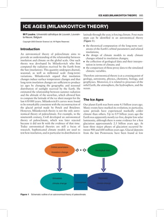
1. ICE AGES (MILANKOVITCH THEORY)
M F Loutre, Universite´ catholique de Louvain, Louvain-
la-Neuve, Belgium
Copyright 2003 Elsevier Science Ltd. All Rights Reserved.
Introduction
An astronomical theory of paleoclimate aims to
provide an understanding of the relationship between
insolation and climate on the global scale. One such
theory was developed by Milankovitch who first
computed the radiation received by the Earth from
the Sun (insolation). This quantity undergoes diurnal,
seasonal, as well as millennial scale (long-term)
variations. Milankovitch argued that insolation
changes induce surface temperature changes and that
long-term insolation changes are sufficient to produce
ice ages by changing the geographic and seasonal
distribution of sunlight received by the Earth. He
estimated the relationship between summer radiation
and the altitude of the snowline, which allowed him
to compute the latitude of the ice sheet margin for the
last 650 000 years. Milankovitch’s curves were found
to be remarkably consistent with the reconstruction of
the glacial period made by Penck and Bru¨ckner.
However, Milankovitch theory is not the only astro-
nomical theory of paleoclimate. For example, in the
nineteenth century, Croll developed an astronomical
theory of paleoclimate, which was later rejected
because it did not fit with the evidence of that time.
Today astronomical theories are still a focus of
research. Sophisticated climate models are used to
test how insolation, and in particular its distribution in
latitude through the year, is forcing climate. Four main
steps can be identified in an astronomical theory
(Figure 1):
the theoretical computation of the long-term vari-
ations of the Earth’s orbital parameters and related
insolations;
the design of climate models to study climate
changes related to insolation changes;
the collection of geological data and their interpre-
tation in terms of climate; and
the comparison of these proxy data to the simulated
climatic variables.
Therefore astronomical theory is at a crossing point of
geology, astronomy, physics, chemistry, biology, and
geophysics. Moreover, it is related to processes of the
solid Earth, the atmosphere, the hydrosphere, and the
ocean.
The Ice Ages
Our planet Earth was born some 4.5 billion years ago.
Many events have marked its evolution; in particular,
some periods have experienced markedly colder
climate than others. Up to 0.9 billion years ago the
Earth was apparently mostly ice-free, despite low solar
luminosity, although there is some evidence for a first
glaciation approximately 2.5 billion years ago. At
least three major phases of glaciation occurred be-
tween 900 and 600 million years ago. Glacial deposits
from the late Proterozoic have been found at low
...Orbital parameters
Insolation change
Geological data
Simulated
climate change
Recorded
climate changeComparison
Figure 1 Schematic outline of an astronomical theory of paleoclimate.
ICE AGES (MILANKOVITCH THEORY) 995

2. latitudes, suggesting that at that time ice sheets
covered the Earth from pole to pole. This is the so-
called ‘snowball Earth’ hypothesis. The return to
warmer conditions would then have resulted from the
accumulation in the atmosphere of CO2 from volcanic
activity. The large cap carbonate found in Namibia,
for example, could be the witness of this time.
However, this hypothesis is still debated. From 600
to 100 million years ago mild climates prevailed,
punctuated by several major phases of ice growth.
These long geological cold periods, such as the late
Precambrian Ice Age, the late Ordovician-Silurian Ice
Age, and the Permo-Carboniferous Ice Age, are also
called Ice Ages. A gradual cooling and drying of the
globe started some 50 million years ago. The Antarctic
ice sheet started to grow some 40 million years ago,
whereas the Greenland and midlatitude ice sheets
formed later (4–2.4 million years ago). The Quater-
nary Ice Age, the cold period in which we are living, is
characterized by a succession of colder and warmer
periods, the glacial–interglacial cycles. During colder
phases (or ice ages) the ice sheets spread out in the high
latitudes. The purpose of astronomical theory is to
explain these broad climatic features, which charac-
terize not only the Quaternary, but also older periods
including the Early Mesozoic, more than 150 million
years ago.
A Brief History of the Astronomical
Theory of Paleoclimates
The inspiration for the pioneering work on the
astronomical theory of paleoclimate was probably
Louis Agassiz’s lecture about his theory of a Great Ice
Age at a meeting of the Swiss Society of Natural
Sciences, held in Neuchaˆtel in 1837. Only a few years
later, Joseph Adhe´mar proposed an explanation of the
existence of ice ages based on the precession of the
equinoxes. At the same time the French astronomer,
Urbain Leverrier, calculated the changes in the Earth’s
orbit over the last 100 000 years. James Croll would
eventually take Adhe´mar’s idea and put it into an
astronomical theory of climate. Croll’s major hypoth-
esis was that the critical season for producing an ice
age is winter. He determined that the precession of the
equinoxes must play a decisive role in the amount of
sunlight received during winter. Indeed, winter would
be warmer if it occurred when the Earth were closer to
the Sun and it would be colder if the Earth were farther
from the Sun. Moreover, the shape of the Earth’s orbit
could reinforce this effect. He concluded that periods
of greater eccentricity could lead to exceptionally
warm or cold winters. He argued that ice ages
therefore occurred alternately in one hemisphere or
the other during Glacial Epochs, when eccentricity is
large. According to Croll, the last Glacial Epoch began
some 250 000 years ago and ended about 80 000 years
ago. Later, he also took into account the role of the tilt
of the Earth’s axis of rotation. He hypothesized that an
ice age would be more likely to occur when the tilt was
small because the polar regions would then receive less
heat. However, he acknowledged that orbital changes
could only be a triggering mechanism. He identified
the albedo–temperature feedback and the change in
ocean currents as two mechanisms responsible for
amplifying the direct climatic effect of the astronom-
ical forcing. Meanwhile, geologists collected evidence
around the world that several ice ages had occurred in
the past, separated by nonglacial epochs, as predicted
by Croll’s theory. However, with time the majority
of geologists in Europe and America became opposed
to Croll’s theory as more and more new evidence
suggested that the last Glacial Period ended later
than 15 000 years ago, instead of 80 000 years
ago as required by Croll’s astronomical theory. By
the end of the nineteenth century, the theory fell into
disfavor.
The attention of the scientific world was drawn
back to the ice age problem with the publication in
1924 of Milankovitch’s theory. This was the first full
astronomical theory of the Pleistocene ice ages,
including the computation of the orbitally induced
changes in the insolation and climate. According to
Milankovitch’s theory, the summer in northern high
latitudes had to be cold to prevent the winter snow
from melting. In turn this would allow a positive value
in the annual budget of ice, and a positive feedback
cooling would be initiated over the Earth through a
further extension of the snow cover and subsequent
increase of surface albedo. This hypothesis requires
that summer insolation is a minimum in the high
latitude Northern Hemisphere. One of Milankovitch’s
first major contributions consisted of radiation curves
showing past insolation changes at high northern
latitudes (Figure 2). He claimed that each minimum of
these curves should cause an ice age. Comparing
Milankovitch’s curves with the Penck and Bru¨ckner
curve for the succession of European ice ages, Ko¨ppen
and Wegener concluded that the theory matched the
facts amazingly well. Although the timing of the ice
ages and the radiation minima did not agree in detail,
the general pattern of the two curves was quite similar.
But by 1955, the astronomical theory was rejected by
geologists. Indeed, using new techniques for dating
Pleistocene fossils (radiocarbon dating) they showed
that there were more glacial advances during the past
80 000 years (or at least the time interval believed to be
80 000 years) than could be explained by the Milan-
kovitch theory.
996 ICE AGES (MILANKOVITCH THEORY)

3. 60°
65°
70°
75°
600 550 500 450 400 350 300 250 200 150 100 50 0
600 550 500 450 350 300 250 200 150 100400 50 0
Time (ky BP)
500
450
400
600 550 500 450 400 350 300 250 200 150 100 50 0
60°
65°
70°
75°
EquivalentlatitudeEquivalentlatitude
GünzI
GünzII
MindelI
MindelII
RissI
RissII
WurmI
WurmII
WurmIII
(A)
(B)
(C)
Figure 2 The Milankovitch amplitude of the secular variations of the summer radiation at 651 N, (A) after Stockwell and Pelgrim’s, and (B) after Le Verrier and Miskovitch’s astronomical solution.
The ordinate axis in (A) and (B) gives the latitude that receives the same radiation as 651 N for the last 600 ky. Part (C) gives the mean irradiance (W mÀ 2
) according to Berger’s computation.
ICEAGES(MILANKOVITCHTHEORY)997

4. The theory was still largely disputed until the early
1970s. Nevertheless, progress was being made toward
a better understanding of the ice ages, in particular the
Pleistocene. New dating techniques were developed
and accurate climatic interpretation was given to
geological records, such as variation of the oxygen
isotope records of forams in deep sea cores, or
sequences of soils and loess. New evidence was put
forward that major climate changes have accompa-
nied variations in obliquity and precession over the
last 500 000 years. This finding stimulated the revival
of the astronomical theory. Vernekar, Bretagnon,
Berger, and others refined the calculations of orbital
history; geologists obtained new records of past
climate; the improved dating techniques clarified the
detail of the Quaternary time scale; global past climate
changes were reconstructed with better accuracy; and
finally, climate models were designed to test this
theory. Within a few years it became increasingly clear
that major changes in global climate were caused by
changes in the astronomically driven insolation forc-
ing. Moreover, the importance of mechanisms and
processes such as the carbon cycle, vegetation change,
ocean circulation, and dynamics of the cryosphere was
also acknowledged.
Orbital Parameters
The German astronomer Johannes Kepler (1571–
1630) formulated the three laws of planetary motion,
which are satisfied with a high accuracy not only by the
system of planets and Sun, but also by the system of
each set of satellites moving about their primary
planet. They are:
The orbit of each planet is an ellipse with the Sun at
one focus.
The line (the radius vector) joining the Sun to each
planet sweeps out equal areas of its ellipse in equal
times.
The cubes of the semimajor axis of the planetary
orbits are proportional to the squares of the planets’
periods of revolution.
While Kepler gave a description of the orbital motion,
Sir Isaac Newton (1642–1727) defined the law of
gravitation, which is the basis for explaining
the planetary motion. In particular, during its
travel counterclockwise on its orbit around the Sun
(Figure 3), the Earth is sometimes nearer to and
sometimes farther away from the Sun. The distance
from the Earth to the Sun (r) can be computed through
the equation of the ellipse, given here as eqn [1].
r ¼ ½að1 À e2
ÞŠÂð1 þ e cos vÞÀ1
½1Š
In eqn [1], a, the semimajor axis of the orbit, gives its
size. The value of a is constant through geological time
to a very good accuracy. The eccentricity, e, is a
measure of the departure of the ellipse from a circle,
and the true anomaly, v, of the Earth is a measure of the
position of the Earth in its orbit. The true anomaly is
measured counterclockwise from perihelion (where
the Earth is nearest to the Sun). Usually the angles that
describe the position of the Earth in its orbit are not
measured from the perihelion, but rather from the
spring equinox (SE). Therefore, we have v ¼ l À o,
where l is the longitude of the Earth in its orbit
measured from the spring equinox of the year, or
moving spring equinox, and o is the longitude of the
perihelion relative to this same moving spring equi-
nox. Alternatively, the position of the perihelion
(oo) is often measured from the First Point of Aries
(vernal point). This point on the Earth’s orbit gives the
direction of the Sun as seen from the Earth at the spring
equinox. Consequently, we have v ¼ l À oo À p. In
addition, the Earth’s axis of rotation is tilted with
respect to the orbital plane. The obliquity, e, is the
angle between the Earth’s axis of rotation and the
perpendicular to the orbital plane.
The astronomical parameters, e, e, and o, experi-
ence long-term variations. These variations can be
obtained by solving two sets of equations, one set for
the mutual gravitational forces in the planetary system
and the other for the Sun–Earth–Moon system.
AE
SS
A
SE
WS
v
S
P
Figure 3 Elements of the Earth’s orbit around the Sun (S). Some
reference points are drawn on the orbit, i.e., the perihelion (P) and
the aphelion (A), the spring equinox (SE), the summer solstice
(SS), the autumn equinox (AE), and the winter solstice (WS). The
vernal point is given by g. l is the longitude of the Earth in its orbit
measured from the spring equinox of the year, or moving spring
equinox; o is the longitude of the perihelion relative to this same
moving spring equinox; and v is the true anomaly measured
counterclockwise from the perihelion.
998 ICE AGES (MILANKOVITCH THEORY)

5. Different methods, from fully analytical to fully
numerical, were developed following the first calcula-
tions by Leverrier in the nineteenth century. Moreover,
the accuracy of these solutions has been greatly
improved. However, the orbital motion of the planets
in the solar system is chaotic, i.e., the solution is
strongly dependent on the initial conditions, which
limits the possibility of obtaining an accurate solution
for the astronomical parameters of the Earth over
more than 35–50 million years.
Figure 4 shows the long-term variations of the three
orbital parameters (e, e, e sin oo) from 400 000 years
Before Present (400 ky BP) to 100 000 years After
Present (100 ky AP), a time slice over which the
solution is very accurate. The eccentricity of the orbit
varies between near circularity (e ¼ 0) and small
ellipticity (e ¼ 0:07). These variations are quasi-peri-
odic with a mean period of about 100 ky. However, a
longer period of about 400 ky can also be discerned. In
practice, the analytical solution for the eccentricity,
expressed in trigonometrical series, puts forwards
many terms having different periods. The major
periods in the development are 404, 95, 124, 99,
and 131 ky (in order of decreasing amplitude). The
obliquity (tilt of the Earth’s axis) varies between 221
and 251 with a very clear quasi-period of 41 ky. The
largest amplitude terms correspond to periods of 41
(by far the largest term), 54, and 39 ky. The variations
of the climatic precession (e sin oo) reflect two oppos-
ing motions, i.e., the counterclockwise motion of the
perihelion along the ecliptic with a period of $ 100 ky
and the clockwise motion of the vernal point along the
ecliptic with a period of $ 25 700 years. The two
effects taken together result in the climatic precession,
which corresponds to the slow shift of the seasons
about the Earth’s orbit relative to the perihelion. This
motion has a mean quasi-period of 21 ky, which is
derived from periods at 19 and 23 ky.
Insolation
The amount of solar radiation received at a mean
Earth–Sun distance, rm, by a surface perpendicular to
the incident radiation, is about 1370 W mÀ 2
(this is the
so-called total solar irradiance, S0). However, rm varies
over time according to the eccentricity. Therefore,
instead of S0, it is often preferred to use the related
quantity, S, defined at the constant distance a from
Sun. As the solar energy decreases according to the
square of the distance from the Sun, the amount of
solar radiation received by the Earth on a unit surface
perpendicular to the Sun’s rays at a distance r from the
_400_350_300_250_200_150_100_50050100
(kyr AP) (kyr BP)
0.00
0.01
0.02
0.03
0.04
0.05
0.06
_
0.02
_
0.04
_
0.06
0.00
0.02
0.04
0.06
22
23
24
25
Obliquity ( )
Climatic precession (e sin )
Eccentricity (e)
Time
_
Figure 4 Long-term variations of eccentricity, climatic precession and obliquity from 400 000 years ago to 100 000 years into the future
(from Berger).
ICE AGES (MILANKOVITCH THEORY) 999

6. Sun is given by W ¼ Sða=rÞ2
. Moreover, the incident
radiation is usually not perpendicular to the Earth’s
surface, but it is tilted according to the elevation of the
Sun above the horizon. The elevation angle at a given
point on the Earth is measured by the zenith distance,
z, which is the angular distance from the zenith (the
point vertically overhead) along the vertical circle
through the point. The instantaneous insolation (irra-
diance) received by a unit horizontal surface at a
particular time characterized by a zenith distance, z, is
given by eqn [2].
W ¼ Sða=rÞ2
cos z ½2Š
Spherical trigonometry applied to the astronomical
coordinates on the celestial sphere for the Earth’s
orbital motion provides cos z (Figure 5), expressed as
eqn [3].
cos z ¼ sin f sin d þ cos f cos d cos H ½3Š
Here f is the latitude on the Earth, d is the declination
(the angular distance from the Equator along the
meridian), and H is the hour angle (measured clock-
wise on the Equator from the meridian of the observer
to the meridian of the Sun). The declination depends
on the obliquity (e). It can be computed for any given
time in the year l using eqn [4].
sin d ¼ sin l sin e ½4Š
This shows that the energy (irradiance) available at
any given latitude f on the Earth (on the assumption of
a perfectly transparent atmosphere) is a single-valued
function of the total solar irradiance, S, the semimajor
axis, a, of the Earth orbit about the Sun, its eccentricity
e, its obliquity e, and the longitude of the perihelion
measured from the moving spring equinox, o. There-
fore it appears that the irradiance varies only accord-
ing to three astronomical parameters, i.e., the
eccentricity (e), the climatic precession (e sin oo) and
the obliquity (e). Moreover, climatic precession and
eccentricity on one side, and obliquity on the other
side, appear in two distinct factors in the formulation
for the irradiance. Each of these factors has a physical
meaning. The distance factor (r ¼ r=a) depends on the
precession and eccentricity, and the inclination factor
(cos z) is solely a function of the obliquity.
The daily irradiation is the irradiance integrated
over a whole day, either from sunrise to sunset or over
24 h, in case of no sunset. The 24 h mean irradiance
(Wd), i.e., the average daily irradiation over 24 h,
expressed in W mÀ 2
, is often preferred. The value of
Wd depends on the latitude.
H
orizon
Equator
Ecliptic
N
PS
PN
SE
S
Z
O
H
z
π
2
_
π
2
_
Figure 5 Position of a celestial body (the Sun for example) on the celestial sphere. The different variables are explained in the text.
1000 ICE AGES (MILANKOVITCH THEORY)

7. For the latitudes where there is a daily sunrise and
sunset, i.e., jfj p=2 À jdj, Wd is expressed by eqn
[5],
Wd ¼ S=prÀ2
ðH0 sin f sin d
þ cos f cos d sin H0Þ ½5Š
where H0, the absolute value of the hour angle at
sunrise and sunset, is given by eqn [6].
cos H0 ¼ À tan f tan d ½6Š
For the other latitudes, i.e., jfj p=2 À jdj:
Either it is the long polar night (H0 ¼ 0), i.e.,
fd 0, in which case Wd is given by [7]
Wd ¼ 0 ½7Š
Or it is the long polar day (H0 ¼ p), i.e., fd 0, in
which case Wd is given by [8].
Wd ¼ SrÀ2
sin f sin d ½8Š
The daily irradiation varies through the year as well
as according to the latitude. Moreover, it also exhibits
long-period variations caused by the secular variations
in the elements of the Earth’s orbit and rotation.
Some features of the long-term variations in eccen-
tricity, obliquity, and climatic precession can be
discerned in the insolation variations. Low values of
the eccentricity are mirrored in the small amplitude of
the insolation change, such as for the recent past and
near future; conversely, large values of e induce large
amplitudes of the insolation change, for example, at
about 100 ky BP (Figure 2C). Solar radiation is mostly
affected by variations in precession, although the
obliquity plays a relatively more important role for
high latitudes, mainly in the winter hemisphere. The
variations in the obliquity are perceptible in the same
way in both hemispheres (Figure 6A), i.e., an increase
in the obliquity induces an increase in the insolation
during the local summer (March to September in the
Northern Hemisphere and September to March in the
Southern Hemisphere) and an insolation decrease
during local winter. Consequently the seasonal con-
trast in daily irradiation is reinforced. A change in the
climatic precession (Figure 6B) such that the June
summer solstice is moving from the perihelion to the
aphelion (i.e., close to the present-day situation)
induces a decrease of insolation over the whole Earth
(Northern and Southern Hemispheres) simultaneous-
ly over one half of the year (Northern Hemisphere
summer season and Southern Hemisphere winter
season, i.e., from March to September). Climatic
precession plays an opposite role in both hemispheres.
At present, perihelion occurs in early January. This
situation favors mild winters and cool summers in the
Northern Hemisphere, and cold winters and warm
summers in the Southern Hemisphere.
Comparison between changes in the orbital param-
eters and/or in the solar radiation received by the Earth
with geological reconstruction of past climate changes
is also used to provide a clock for dating the records. In
this case it is assumed that the quasi-periods observed
in the data are a direct response to the quasi-periodic
variations of the forcing. Consequently the astronom-
ical chronology is directly applied to the geological
data, possibly with a time lag.
90° N
60° N
30° N
30° S
60° S
90° S
0°
Latitude
Jan Feb Mar Apr May Jun Jul Aug Sep Oct Nov Dec
Time (month)
_100 _80 _60 _40 _20 0 20 40 60 80 100(B)
Jan Feb Mar Apr May Jun Jul Aug Sep Oct Nov Dec
Time (month)
90° N
60° N
30° N
30° S
60° S
90° S
0°
Latitude
_20 _10 0 10 20 30 40 50 60(A)
Figure 6 Variation of the seasonal contrast of the mean irradiance (W mÀ 2
) following (A) an increase of the obliquity from 22.51 to 251
(e ¼ 0:05 and winter at perihelion) and (B) a change in the climatic precession (from summer solstice at perihelion to summer solstice at
aphelion; e ¼ 0:05 and e ¼ 25
).
ICE AGES (MILANKOVITCH THEORY) 1001

8. Paleoclimate Modeling
Climate models are simplifications of reality, designed
to describe the complexity of the interactions within
the climate system. These numerical climate models
can be used to test the astronomical theory of
paleoclimate, i.e., to study whether astronomically
induced changes in insolation are able to drive
the climate system into glacial–interglacial cycles
similar to these recorded in geological data. The
modeling effort has led to a better understanding of the
physical mechanisms involved in the climate system
response to the astronomically forced changes in the
pattern of incoming solar radiation. Such mechanisms
are related, in particular, to the ice sheets, the
lithosphere, the hydrological cycle, the cloud proper-
ties, the albedo temperature feedback, the land–sea ice
temperature gradient, the CO2 cycle, and the ocean
circulation. The different parts of the climate system,
i.e., the atmosphere, the hydrosphere, the cryosphere,
the biosphere, and the lithosphere, are becoming
convincingly modeled separately, and work is going
on towards the design of comprehensive coupled
models including several parts, if not all of them. A
hierarchy of models, climate models of different
complexities that differ in their degree of spatial and
temporal resolution, are used for paleoclimate
purposes.
General Circulation Models (GCMs) are primarily
used for simulating geographic features of paleocli-
mates. Their major limitation is their high computing
cost. For this reason they are used for simulations
covering a few thousand years at maximum. They
provide a ‘snapshot’ view of the climate in equilibrium
with the boundary conditions.
At the last interglacial, some 125 ky BP, modeling
experiments led to warmer conditions, especially in
the high latitudes, reduced sea-ice extent, enhanced
northern tropical monsoon and northward displace-
ment of the tundra and taiga biomes, in good agree-
ment with geological reconstruction. However, the
strong cooling induced by changes in the orbital
parameters at 115 ky BP are not sufficient to initiate
glaciation, at least if vegetation changes are not
properly taken into account. This clearly puts forward
the importance of the vegetation–albedo–temperature
feedback. Several GCMs have been used to simulate
the climate of the Last Glacial Maximum, some 20 ky
ago. Again, important processes at work at that time
were identified. They are related to the CO2 concen-
tration, sea ice, ocean temperature, and land albedo.
As part of the Paleoclimate Modeling Intercomparison
Project (PMIP), several GCMs performed the same
simulation of the mid-Holocene climate (6 ky BP).
Some robust features have been identified, for instance
a northward shift of the main regions of monsoon
precipitation over Africa and India.
The conceptual models are simple models designed
to assess whether a climate process can explain
past climate changes. For example, the simple thresh-
old (or multistate) climate model due to Paillard
simulates ice volume increase as a function of a
smoothed truncation of the insolation. The
model distinguishes three distinct states (interglacial,
mild glacial, and full glacial) and the transition
between them occurs when insolation and ice volume
cross prescribed thresholds in insolation and ice
volume. This model reproduced reasonably well the
succession of glacial–interglacial cycles over the late
Pleistocene.
Models of intermediate complexity are the only
climate models to be able to simulate the time-
dependent behavior of the fully coupled climate
system over a time interval long enough to test the
astronomical theory of paleoclimate. Earth system
Models of Intermediate Complexity (EMICs) include
most of the processes described in comprehensive
models, in particular the slow-response climate vari-
ables such as ice volume, bedrock depression, deep-
ocean temperature, and atmospheric concentration of
greenhouse gases. They also simulate the interactions
between the different parts of the climate system.
Moreover, they are simple enough to allow for long-
term climate simulations (several glacial–interglacial
cycles).
The LLN 2D NH climate model (two-dimensional
climate model developed in Louvain-la-Neuve) is one
of these EMICs. It was designed in order to understand
the response of the climate system to astronomical
forcing. It links the atmosphere, the upper mixed layer
of the ocean, the sea ice, the continents, the ice sheets,
and their underlying lithosphere. It is forced by
computed insolation and reconstructed atmospheric
CO2 concentration. It considers only the Northern
Hemisphere (the Southern Hemisphere is not consid-
ered) and it has no explicit representation of the
thermohaline circulation. It has been able to simulate
many of the different situations that characterize the
last 3 million years: the entrance into glaciation
around 2.75 My BP, the dominance of the obliquity
cycle during the late Pliocene–early Pleistocene, the
emergence of the 100 ky cycle around 900 ky BP, and
the glacial–interglacial cycles of the last 600 ky. The
climatic changes over the Northern Hemisphere, in
particular the continental ice volume, simulated by the
LLN 2D NH climate model during the last 400 ky
shows a broad good agreement with reconstruction
(Figure 7).
However, a major discrepancy in this model is the
too frequent melting of the ice sheets during the
1002 ICE AGES (MILANKOVITCH THEORY)

9. interglacial. The largest difference between the simu-
lated and the reconstructed Northern Hemisphere
continental ice volume appears between 180 and
150 ky BP. Moreover an unusual feature shows up
between 400 and 350 ky BP. This time interval is
characterized by a very long interglacial, which
does not seem to be recorded in data. This behavior
is possibly caused by the interplay between insolation
forcing and CO2 concentration forcing. This
model also confirms that the orbital forcing acts
as a pacemaker for the glacial–interglacial cycles
and that the climate response to orbital forcing is
amplified by CO2. Moreover, important processes in
climate change were identified, such as albedo–
temperature feedback, water vapor–temperature feed-
back, the snow aging process, and the isostatic
rebound.
New observation techniques, accurate dating meth-
ods, improved transfer functions, and comprehensive
climate models will lead to increasingly accurate
knowledge of the past evolution of the atmosphere
and the oceans, the waxing and waning of the ice
sheets, and the growth and retreat of the forests and
deserts.
See also
Carbon Dioxide. Climate Variability: Glacial, Intergla-
cial Variations. Energy Balance Model, Surface. Gen-
eral Circulation: Models. Glaciers. Numerical
Models: Methods. Paleoclimatology: Ice Cores;Varves.
Further Reading
Berger A, Imbrie J, Hays J, Kukla G and Saltzman B (eds)
(1984) Milankovitch and Climate. NATO ASI Series C,
vol. 126. Dordrecht: Reidel Publishing Company.
Bradley R (1999) Paleoclimatology. Reconstructing
Climates of the Quaternary. New York and London:
Academic Press.
Imbrie J and Imbrie KP (1979) Ice Ages. Solving the Mystery.
Cambridge, MA and London, England: Harvard Univer-
sity Press.
Milankovitch MM (1941) Kanon der Erdbestrahlung
und seine Anwendung auf des Eizeitenproblem.
R. Serbian Acad. Spec. Publ. 132, Sect. Math. Nat.
Sci., 33. Beograd: Ko¨ninglich Serbische Akademie.
Reprinted in English: Canon of Insolation and the
Ice-Age Problem. Zavod za udzbenikb i nastavna
sredstva, Beograd (1998).
Roy AE (1978) Orbital Motion. Bristol, Philadelphia and
New York: Adam Hilger.
400350300250200150100500
Age (ky BP)
200
250
CO2
(ppmv)
450
Insolation(Wm
_2
)
500
550
_2
0
2
δ
18
O 0
10
20
30
40
50
Icevolume(106km3)
Sealevel
(A)
(B)
(C)
Figure 7 Comparison of records and modeled data over the last 400 000 years. (A) Variation in the mean irradiance in July at 601 N (red
full line) and the CO2 concentration (dashed green line). (B) Proxy records for the variation of continental ice volume, i.e., stacked,
smoothed oxygen isotope record as function of age in the SPECMAP time scale (full dark blue line), d18
O record from the oceanic core
MD900963 (long-dashed blue line), and reconstructed sea level from benthic forams in the oceanic core V19-30 (short-dashed blue line).
(C) Northern Hemisphere continental volume as simulated by the LLN 2D NH climate model.
ICE AGES (MILANKOVITCH THEORY) 1003