Download as PDF, PPTX


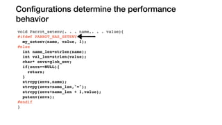
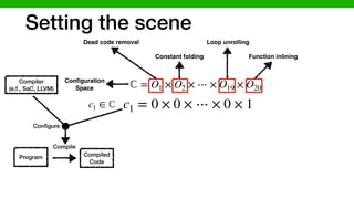
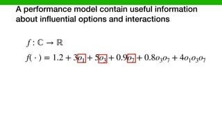
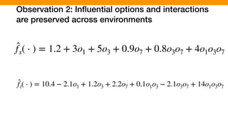
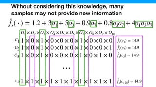
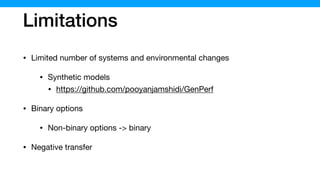
![Empirical observations confirm that systems are
becoming increasingly configurable
08 7/2010 7/2012 7/2014
Release time
1/1999 1/2003 1/2007 1/2011
0
1/2014
N
Release time
02 1/2006 1/2010 1/2014
2.2.14
2.3.4
2.0.35
.3.24
Release time
Apache
1/2006 1/2008 1/2010 1/2012 1/2014
0
40
80
120
160
200
2.0.0
1.0.0
0.19.0
0.1.0
Hadoop
Numberofparameters
Release time
MapReduce
HDFS
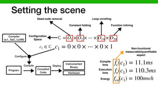
[Tianyin Xu, et al., “Too Many Knobs…”, FSE’15]](https://image.slidesharecdn.com/talk-pooyan-furman2-190416181547/85/Transfer-Learning-for-Performance-Analysis-of-Machine-Learning-Systems-23-320.jpg)
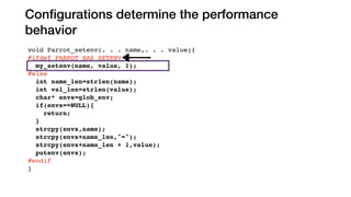
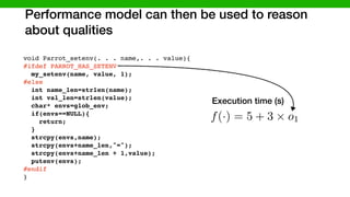
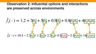
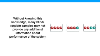
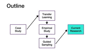
![Empirical observations confirm that systems are
becoming increasingly configurable
nia San Diego, ‡Huazhong Univ. of Science & Technology, †NetApp, Inc
tixu, longjin, xuf001, yyzhou}@cs.ucsd.edu
kar.Pasupathy, Rukma.Talwadker}@netapp.com
prevalent, but also severely
software. One fundamental
y of configuration, reflected
parameters (“knobs”). With
m software to ensure high re-
aunting, error-prone task.
nderstanding a fundamental
users really need so many
answer, we study the con-
including thousands of cus-
m (Storage-A), and hundreds
ce system software projects.
ng findings to motivate soft-
ore cautious and disciplined
these findings, we provide
ich can significantly reduce
A as an example, the guide-
ters and simplify 19.7% of
on existing users. Also, we
tion methods in the context
7/2006 7/2008 7/2010 7/2012 7/2014
0
100
200
300
400
500
600
700
Storage-A
Numberofparameters
Release time
1/1999 1/2003 1/2007 1/2011
0
100
200
300
400
500
5.6.2
5.5.0
5.0.16
5.1.3
4.1.0
4.0.12
3.23.0
1/2014
MySQL
Numberofparameters
Release time
1/1998 1/2002 1/2006 1/2010 1/2014
0
100
200
300
400
500
600
1.3.14
2.2.14
2.3.4
2.0.35
1.3.24
Numberofparameters
Release time
Apache
1/2006 1/2008 1/2010 1/2012 1/2014
0
40
80
120
160
200
2.0.0
1.0.0
0.19.0
0.1.0
Hadoop
Numberofparameters
Release time
MapReduce
HDFS
[Tianyin Xu, et al., “Too Many Knobs…”, FSE’15]](https://image.slidesharecdn.com/talk-pooyan-furman2-190416181547/85/Transfer-Learning-for-Performance-Analysis-of-Machine-Learning-Systems-24-320.jpg)


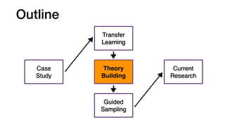
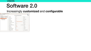
![Outline
Case
Study
Transfer
Learning
[SEAMS’17]](https://image.slidesharecdn.com/talk-pooyan-furman2-190416181547/85/Transfer-Learning-for-Performance-Analysis-of-Machine-Learning-Systems-35-320.jpg)
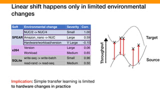
![Outline
Case
Study
Transfer
Learning
Theory
Building
[SEAMS’17]
[ASE’17]](https://image.slidesharecdn.com/talk-pooyan-furman2-190416181547/85/Transfer-Learning-for-Performance-Analysis-of-Machine-Learning-Systems-36-320.jpg)
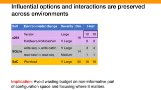
![Outline
Case
Study
Transfer
Learning
Theory
Building
Guided
Sampling
[SEAMS’17]
[ASE’17]
[FSE’18]](https://image.slidesharecdn.com/talk-pooyan-furman2-190416181547/85/Transfer-Learning-for-Performance-Analysis-of-Machine-Learning-Systems-37-320.jpg)
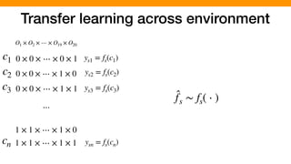
![Outline
Case
Study
Transfer
Learning
Theory
Building
Guided
Sampling
Current
Research
[SEAMS’17]
[ASE’17]
[FSE’18]](https://image.slidesharecdn.com/talk-pooyan-furman2-190416181547/85/Transfer-Learning-for-Performance-Analysis-of-Machine-Learning-Systems-38-320.jpg)
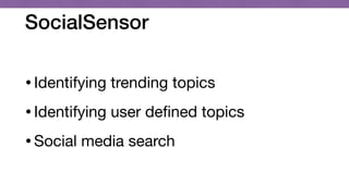

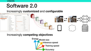
![SocialSensor
Crawling
Tweets: [5k-20k/min]
Crawled
items
Internet](https://image.slidesharecdn.com/talk-pooyan-furman2-190416181547/85/Transfer-Learning-for-Performance-Analysis-of-Machine-Learning-Systems-41-320.jpg)
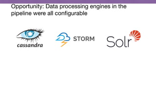
![SocialSensor
Crawling
Tweets: [5k-20k/min]
Store
Crawled
items
Internet](https://image.slidesharecdn.com/talk-pooyan-furman2-190416181547/85/Transfer-Learning-for-Performance-Analysis-of-Machine-Learning-Systems-42-320.jpg)
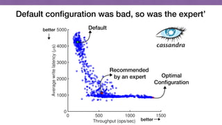
![SocialSensor
Orchestrator
Crawling
Tweets: [5k-20k/min]
Every 10 min:
[100k tweets]
Store
Crawled
items
FetchInternet](https://image.slidesharecdn.com/talk-pooyan-furman2-190416181547/85/Transfer-Learning-for-Performance-Analysis-of-Machine-Learning-Systems-43-320.jpg)
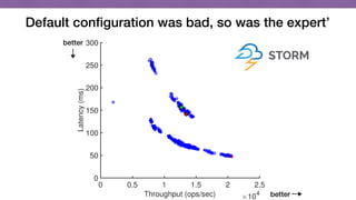
![SocialSensor
Content AnalysisOrchestrator
Crawling
Tweets: [5k-20k/min]
Every 10 min:
[100k tweets]
Store
Push
Crawled
items
FetchInternet](https://image.slidesharecdn.com/talk-pooyan-furman2-190416181547/85/Transfer-Learning-for-Performance-Analysis-of-Machine-Learning-Systems-44-320.jpg)
![SocialSensor
Content AnalysisOrchestrator
Crawling
Tweets: [5k-20k/min]
Every 10 min:
[100k tweets]
Tweets: [10M]
Store
Push
Store
Crawled
items
FetchInternet](https://image.slidesharecdn.com/talk-pooyan-furman2-190416181547/85/Transfer-Learning-for-Performance-Analysis-of-Machine-Learning-Systems-45-320.jpg)
![SocialSensor
Content AnalysisOrchestrator
Crawling
Search and Integration
Tweets: [5k-20k/min]
Every 10 min:
[100k tweets]
Tweets: [10M]
Fetch
Store
Push
Store
Crawled
items
FetchInternet](https://image.slidesharecdn.com/talk-pooyan-furman2-190416181547/85/Transfer-Learning-for-Performance-Analysis-of-Machine-Learning-Systems-46-320.jpg)
![Challenges
Content AnalysisOrchestrator
Crawling
Search and Integration
Tweets: [5k-20k/min]
Every 10 min:
[100k tweets]
Tweets: [10M]
Fetch
Store
Push
Store
Crawled
items
FetchInternet](https://image.slidesharecdn.com/talk-pooyan-furman2-190416181547/85/Transfer-Learning-for-Performance-Analysis-of-Machine-Learning-Systems-47-320.jpg)
![Challenges
Content AnalysisOrchestrator
Crawling
Search and Integration
Tweets: [5k-20k/min]
Every 10 min:
[100k tweets]
Tweets: [10M]
Fetch
Store
Push
Store
Crawled
items
FetchInternet
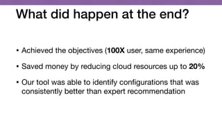
100X](https://image.slidesharecdn.com/talk-pooyan-furman2-190416181547/85/Transfer-Learning-for-Performance-Analysis-of-Machine-Learning-Systems-48-320.jpg)
![Challenges
Content AnalysisOrchestrator
Crawling
Search and Integration
Tweets: [5k-20k/min]
Every 10 min:
[100k tweets]
Tweets: [10M]
Fetch
Store
Push
Store
Crawled
items
FetchInternet
100X
10X](https://image.slidesharecdn.com/talk-pooyan-furman2-190416181547/85/Transfer-Learning-for-Performance-Analysis-of-Machine-Learning-Systems-49-320.jpg)
![Challenges
Content AnalysisOrchestrator
Crawling
Search and Integration
Tweets: [5k-20k/min]
Every 10 min:
[100k tweets]
Tweets: [10M]
Fetch
Store
Push
Store
Crawled
items
FetchInternet
100X
10X
Real time](https://image.slidesharecdn.com/talk-pooyan-furman2-190416181547/85/Transfer-Learning-for-Performance-Analysis-of-Machine-Learning-Systems-50-320.jpg)


![We developed methods to make learning cheaper
via transfer learning
Target (Learn)Source (Given)
DataModel
Transferable
Knowledge
II. INTUITION
Understanding the performance behavior of configurable
software systems can enable (i) performance debugging, (ii)
performance tuning, (iii) design-time evolution, or (iv) runtime
adaptation [11]. We lack empirical understanding of how the
performance behavior of a system will vary when the environ-
ment of the system changes. Such empirical understanding will
provide important insights to develop faster and more accurate
learning techniques that allow us to make predictions and
optimizations of performance for highly configurable systems
in changing environments [10]. For instance, we can learn
performance behavior of a system on a cheap hardware in a
controlled lab environment and use that to understand the per-
formance behavior of the system on a production server before
shipping to the end user. More specifically, we would like to
know, what the relationship is between the performance of a
system in a specific environment (characterized by software
configuration, hardware, workload, and system version) to the
one that we vary its environmental conditions.
In this research, we aim for an empirical understanding of
A. Preliminary concept
In this section, we p
cepts that we use throu
enable us to concisely
1) Configuration and
the i-th feature of a co
enabled or disabled an
configuration space is m
all the features C =
Dom(Fi) = {0, 1}. A
a member of the confi
all the parameters are
range (i.e., complete ins
We also describe an
e = [w, h, v] drawn fr
W ⇥H ⇥V , where they
values for workload, ha
2) Performance mod
configuration space F
formance model is a b
given some observation
combination of system
II. INTUITION
rstanding the performance behavior of configurable
systems can enable (i) performance debugging, (ii)
ance tuning, (iii) design-time evolution, or (iv) runtime
on [11]. We lack empirical understanding of how the
ance behavior of a system will vary when the environ-
the system changes. Such empirical understanding will
important insights to develop faster and more accurate
techniques that allow us to make predictions and
ations of performance for highly configurable systems
ging environments [10]. For instance, we can learn
ance behavior of a system on a cheap hardware in a
ed lab environment and use that to understand the per-
e behavior of the system on a production server before
to the end user. More specifically, we would like to
hat the relationship is between the performance of a
n a specific environment (characterized by software
ation, hardware, workload, and system version) to the
we vary its environmental conditions.
s research, we aim for an empirical understanding of
A. Preliminary concepts
In this section, we provide formal definitions of
cepts that we use throughout this study. The forma
enable us to concisely convey concept throughout
1) Configuration and environment space: Let F
the i-th feature of a configurable system A whic
enabled or disabled and one of them holds by de
configuration space is mathematically a Cartesian
all the features C = Dom(F1) ⇥ · · · ⇥ Dom(F
Dom(Fi) = {0, 1}. A configuration of a syste
a member of the configuration space (feature spa
all the parameters are assigned to a specific valu
range (i.e., complete instantiations of the system’s pa
We also describe an environment instance by 3
e = [w, h, v] drawn from a given environment s
W ⇥H ⇥V , where they respectively represent sets
values for workload, hardware and system version.
2) Performance model: Given a software syste
configuration space F and environmental instances
formance model is a black-box function f : F ⇥
given some observations of the system performanc
combination of system’s features x 2 F in an en
formance model is a black-box function f : F ⇥ E ! R
given some observations of the system performance for each
combination of system’s features x 2 F in an environment
e 2 E. To construct a performance model for a system A
with configuration space F, we run A in environment instance
e 2 E on various combinations of configurations xi 2 F, and
record the resulting performance values yi = f(xi) + ✏i, xi 2
F where ✏i ⇠ N (0, i). The training data for our regression
models is then simply Dtr = {(xi, yi)}n
i=1. In other words, a
response function is simply a mapping from the input space to
a measurable performance metric that produces interval-scaled
data (here we assume it produces real numbers).
3) Performance distribution: For the performance model,
we measured and associated the performance response to each
configuration, now let introduce another concept where we
vary the environment and we measure the performance. An
empirical performance distribution is a stochastic process,
pd : E ! (R), that defines a probability distribution over
performance measures for each environmental conditions. To
tem version) to the
ons.
al understanding of
g via an informed
learning a perfor-
ed on a well-suited
the knowledge we
the main research
information (trans-
o both source and
ore can be carried
r. This transferable
[10].
s that we consider
uration is a set of
is the primary vari-
rstand performance
ike to understand
der study will be
formance model is a black-box function f : F ⇥ E
given some observations of the system performance fo
combination of system’s features x 2 F in an enviro
e 2 E. To construct a performance model for a syst
with configuration space F, we run A in environment in
e 2 E on various combinations of configurations xi 2 F
record the resulting performance values yi = f(xi) + ✏i
F where ✏i ⇠ N (0, i). The training data for our regr
models is then simply Dtr = {(xi, yi)}n
i=1. In other wo
response function is simply a mapping from the input sp
a measurable performance metric that produces interval-
data (here we assume it produces real numbers).
3) Performance distribution: For the performance m
we measured and associated the performance response t
configuration, now let introduce another concept whe
vary the environment and we measure the performanc
empirical performance distribution is a stochastic pr
pd : E ! (R), that defines a probability distributio
performance measures for each environmental conditio
Extract Reuse
Learn Learn
Goal: Gain strength by
transferring information
across environments](https://image.slidesharecdn.com/talk-pooyan-furman2-190416181547/85/Transfer-Learning-for-Performance-Analysis-of-Machine-Learning-Systems-105-320.jpg)


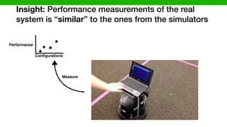
![TurtleBot
[P. Jamshidi, et al., “Transfer learning for improving model predictions ….”, SEAMS’17]
Our transfer learning solution](https://image.slidesharecdn.com/talk-pooyan-furman2-190416181547/85/Transfer-Learning-for-Performance-Analysis-of-Machine-Learning-Systems-109-320.jpg)
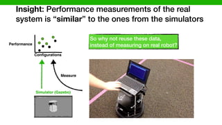
![TurtleBot
Simulator (Gazebo)
[P. Jamshidi, et al., “Transfer learning for improving model predictions ….”, SEAMS’17]
Our transfer learning solution](https://image.slidesharecdn.com/talk-pooyan-furman2-190416181547/85/Transfer-Learning-for-Performance-Analysis-of-Machine-Learning-Systems-110-320.jpg)
![Data
Measure
TurtleBot
Simulator (Gazebo)
[P. Jamshidi, et al., “Transfer learning for improving model predictions ….”, SEAMS’17]
Our transfer learning solution](https://image.slidesharecdn.com/talk-pooyan-furman2-190416181547/85/Transfer-Learning-for-Performance-Analysis-of-Machine-Learning-Systems-111-320.jpg)
![DataData
Data
Measure
Measure
Reuse
TurtleBot
Simulator (Gazebo)
[P. Jamshidi, et al., “Transfer learning for improving model predictions ….”, SEAMS’17]
Configurations
Our transfer learning solution](https://image.slidesharecdn.com/talk-pooyan-furman2-190416181547/85/Transfer-Learning-for-Performance-Analysis-of-Machine-Learning-Systems-112-320.jpg)
![DataData
Data
Measure
Measure
Reuse Learn
TurtleBot
Simulator (Gazebo)
[P. Jamshidi, et al., “Transfer learning for improving model predictions ….”, SEAMS’17]
Configurations
Our transfer learning solution
f(o1, o2) = 5 + 3o1 + 15o2 7o1 ⇥ o2](https://image.slidesharecdn.com/talk-pooyan-furman2-190416181547/85/Transfer-Learning-for-Performance-Analysis-of-Machine-Learning-Systems-113-320.jpg)


![CoBot experiment: DARPA BRASS
0 2 4 6 8
Localization error [m]
10
15
20
25
30
35
40
CPUutilization[%]
Pareto
front
better
better
no_of_particles=x
no_of_refinement=y](https://image.slidesharecdn.com/talk-pooyan-furman2-190416181547/85/Transfer-Learning-for-Performance-Analysis-of-Machine-Learning-Systems-124-320.jpg)
![CoBot experiment: DARPA BRASS
0 2 4 6 8
Localization error [m]
10
15
20
25
30
35
40
CPUutilization[%]
Energy
constraint
Pareto
front
better
better
no_of_particles=x
no_of_refinement=y](https://image.slidesharecdn.com/talk-pooyan-furman2-190416181547/85/Transfer-Learning-for-Performance-Analysis-of-Machine-Learning-Systems-125-320.jpg)
![CoBot experiment: DARPA BRASS
0 2 4 6 8
Localization error [m]
10
15
20
25
30
35
40
CPUutilization[%]
Energy
constraint
Safety
constraint
Pareto
front
better
better
no_of_particles=x
no_of_refinement=y](https://image.slidesharecdn.com/talk-pooyan-furman2-190416181547/85/Transfer-Learning-for-Performance-Analysis-of-Machine-Learning-Systems-126-320.jpg)
![CoBot experiment: DARPA BRASS
0 2 4 6 8
Localization error [m]
10
15
20
25
30
35
40
CPUutilization[%]
Energy
constraint
Safety
constraint
Pareto
front
Sweet
Spot
better
better
no_of_particles=x
no_of_refinement=y](https://image.slidesharecdn.com/talk-pooyan-furman2-190416181547/85/Transfer-Learning-for-Performance-Analysis-of-Machine-Learning-Systems-127-320.jpg)
![CoBot
experiment
5 10 15 20 25
5
10
15
20
25
0
5
10
15
20
25
Source
(given)
CPU [%]](https://image.slidesharecdn.com/talk-pooyan-furman2-190416181547/85/Transfer-Learning-for-Performance-Analysis-of-Machine-Learning-Systems-129-320.jpg)
![CoBot
experiment
5 10 15 20 25
5
10
15
20
25
0
5
10
15
20
25
5 10 15 20 25
5
10
15
20
25
0
5
10
15
20
25
Source
(given)
Target
(ground truth
6 months)
CPU [%] CPU [%]](https://image.slidesharecdn.com/talk-pooyan-furman2-190416181547/85/Transfer-Learning-for-Performance-Analysis-of-Machine-Learning-Systems-130-320.jpg)
![CoBot
experiment
5 10 15 20 25
5
10
15
20
25
0
5
10
15
20
25
5 10 15 20 25
5
10
15
20
25
0
5
10
15
20
25
5 10 15 20 25
5
10
15
20
25
0
5
10
15
20
25
Source
(given)
Target
(ground truth
6 months)
Prediction with
4 samples
CPU [%] CPU [%]](https://image.slidesharecdn.com/talk-pooyan-furman2-190416181547/85/Transfer-Learning-for-Performance-Analysis-of-Machine-Learning-Systems-131-320.jpg)
![CoBot
experiment
5 10 15 20 25
5
10
15
20
25
0
5
10
15
20
25
5 10 15 20 25
5
10
15
20
25
0
5
10
15
20
25
5 10 15 20 25
5
10
15
20
25
0
5
10
15
20
25
5 10 15 20 25
5
10
15
20
25
0
5
10
15
20
25
Source
(given)
Target
(ground truth
6 months)
Prediction with
4 samples
Prediction with
Transfer learning
CPU [%] CPU [%]](https://image.slidesharecdn.com/talk-pooyan-furman2-190416181547/85/Transfer-Learning-for-Performance-Analysis-of-Machine-Learning-Systems-132-320.jpg)
![Transfer Learning for Improving Model Predictions
in Highly Configurable Software
Pooyan Jamshidi, Miguel Velez, Christian K¨astner
Carnegie Mellon University, USA
{pjamshid,mvelezce,kaestner}@cs.cmu.edu
Norbert Siegmund
Bauhaus-University Weimar, Germany
norbert.siegmund@uni-weimar.de
Prasad Kawthekar
Stanford University, USA
pkawthek@stanford.edu
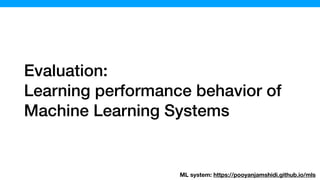
Abstract—Modern software systems are built to be used in
dynamic environments using configuration capabilities to adapt to
changes and external uncertainties. In a self-adaptation context,
we are often interested in reasoning about the performance of
the systems under different configurations. Usually, we learn
a black-box model based on real measurements to predict
the performance of the system given a specific configuration.
However, as modern systems become more complex, there are
many configuration parameters that may interact and we end up
learning an exponentially large configuration space. Naturally,
this does not scale when relying on real measurements in the
actual changing environment. We propose a different solution:
Instead of taking the measurements from the real system, we
learn the model using samples from other sources, such as
simulators that approximate performance of the real system at
Predictive Model
Learn Model with
Transfer Learning
Measure Measure
Data
Source
Target
Simulator (Source) Robot (Target)
Adaptation
Fig. 1: Transfer learning for performance model learning.
order to identify the best performing configuration for a robot
Details: [SEAMS ’17]](https://image.slidesharecdn.com/talk-pooyan-furman2-190416181547/85/Transfer-Learning-for-Performance-Analysis-of-Machine-Learning-Systems-133-320.jpg)
![Looking further: When transfer learning goes
wrong
10
20
30
40
50
60
AbsolutePercentageError[%]
Sources s s1 s2 s3 s4 s5 s6
noise-level 0 5 10 15 20 25 30
corr. coeff. 0.98 0.95 0.89 0.75 0.54 0.34 0.19
µ(pe) 15.34 14.14 17.09 18.71 33.06 40.93 46.75
Insight: Predictions become
more accurate when the source
is more related to the target.
Non-transfer-learning](https://image.slidesharecdn.com/talk-pooyan-furman2-190416181547/85/Transfer-Learning-for-Performance-Analysis-of-Machine-Learning-Systems-135-320.jpg)
![Looking further: When transfer learning goes
wrong
10
20
30
40
50
60
AbsolutePercentageError[%]
Sources s s1 s2 s3 s4 s5 s6
noise-level 0 5 10 15 20 25 30
corr. coeff. 0.98 0.95 0.89 0.75 0.54 0.34 0.19
µ(pe) 15.34 14.14 17.09 18.71 33.06 40.93 46.75
It worked!
Insight: Predictions become
more accurate when the source
is more related to the target.
Non-transfer-learning](https://image.slidesharecdn.com/talk-pooyan-furman2-190416181547/85/Transfer-Learning-for-Performance-Analysis-of-Machine-Learning-Systems-136-320.jpg)
![Looking further: When transfer learning goes
wrong
10
20
30
40
50
60
AbsolutePercentageError[%]
Sources s s1 s2 s3 s4 s5 s6
noise-level 0 5 10 15 20 25 30
corr. coeff. 0.98 0.95 0.89 0.75 0.54 0.34 0.19
µ(pe) 15.34 14.14 17.09 18.71 33.06 40.93 46.75
It worked! It didn’t!
Insight: Predictions become
more accurate when the source
is more related to the target.
Non-transfer-learning](https://image.slidesharecdn.com/talk-pooyan-furman2-190416181547/85/Transfer-Learning-for-Performance-Analysis-of-Machine-Learning-Systems-137-320.jpg)
![5 10 15 20 25
number of particles
5
10
15
20
25
numberofrefinements
5
10
15
20
25
30
5 10 15 20 25
number of particles
5
10
15
20
25
numberofrefinements
10
12
14
16
18
20
22
24
5 10 15 20 25
number of particles
5
10
15
20
25
numberofrefinements
10
15
20
25
5 10 15 20 25
number of particles
5
10
15
20
25
numberofrefinements
10
15
20
25
5 10 15 20 25
number of particles
5
10
15
20
25
numberofrefinements
6
8
10
12
14
16
18
20
22
24
(a) (b) (c)
(d) (e) 5 10 15 20 25
number of particles
5
10
15
20
25
numberofrefinements
12
14
16
18
20
22
24
(f)
CPU usage [%]
CPU usage [%] CPU usage [%]
CPU usage [%] CPU usage [%] CPU usage [%]](https://image.slidesharecdn.com/talk-pooyan-furman2-190416181547/85/Transfer-Learning-for-Performance-Analysis-of-Machine-Learning-Systems-138-320.jpg)
![5 10 15 20 25
number of particles
5
10
15
20
25
numberofrefinements
5
10
15
20
25
30
5 10 15 20 25
number of particles
5
10
15
20
25
numberofrefinements
10
12
14
16
18
20
22
24
5 10 15 20 25
number of particles
5
10
15
20
25
numberofrefinements
10
15
20
25
5 10 15 20 25
number of particles
5
10
15
20
25
numberofrefinements
10
15
20
25
5 10 15 20 25
number of particles
5
10
15
20
25
numberofrefinements
6
8
10
12
14
16
18
20
22
24
(a) (b) (c)
(d) (e) 5 10 15 20 25
number of particles
5
10
15
20
25
numberofrefinements
12
14
16
18
20
22
24
(f)
CPU usage [%]
CPU usage [%] CPU usage [%]
CPU usage [%] CPU usage [%] CPU usage [%]
It worked! It worked! It worked!
It didn’t! It didn’t! It didn’t!](https://image.slidesharecdn.com/talk-pooyan-furman2-190416181547/85/Transfer-Learning-for-Performance-Analysis-of-Machine-Learning-Systems-139-320.jpg)
![Key question: Can we develop a theory to explain
when transfer learning works?
Target (Learn)Source (Given)
DataModel
Transferable
Knowledge
II. INTUITION
rstanding the performance behavior of configurable
e systems can enable (i) performance debugging, (ii)
mance tuning, (iii) design-time evolution, or (iv) runtime
on [11]. We lack empirical understanding of how the
mance behavior of a system will vary when the environ-
the system changes. Such empirical understanding will
important insights to develop faster and more accurate
g techniques that allow us to make predictions and
ations of performance for highly configurable systems
ging environments [10]. For instance, we can learn
mance behavior of a system on a cheap hardware in a
ed lab environment and use that to understand the per-
ce behavior of the system on a production server before
g to the end user. More specifically, we would like to
what the relationship is between the performance of a
in a specific environment (characterized by software
ration, hardware, workload, and system version) to the
t we vary its environmental conditions.
is research, we aim for an empirical understanding of
mance behavior to improve learning via an informed
g process. In other words, we at learning a perfor-
model in a changed environment based on a well-suited
g set that has been determined by the knowledge we
in other environments. Therefore, the main research
A. Preliminary concepts
In this section, we provide formal definitions of four con-
cepts that we use throughout this study. The formal notations
enable us to concisely convey concept throughout the paper.
1) Configuration and environment space: Let Fi indicate
the i-th feature of a configurable system A which is either
enabled or disabled and one of them holds by default. The
configuration space is mathematically a Cartesian product of
all the features C = Dom(F1) ⇥ · · · ⇥ Dom(Fd), where
Dom(Fi) = {0, 1}. A configuration of a system is then
a member of the configuration space (feature space) where
all the parameters are assigned to a specific value in their
range (i.e., complete instantiations of the system’s parameters).
We also describe an environment instance by 3 variables
e = [w, h, v] drawn from a given environment space E =
W ⇥H ⇥V , where they respectively represent sets of possible
values for workload, hardware and system version.
2) Performance model: Given a software system A with
configuration space F and environmental instances E, a per-
formance model is a black-box function f : F ⇥ E ! R
given some observations of the system performance for each
combination of system’s features x 2 F in an environment
e 2 E. To construct a performance model for a system A
with configuration space F, we run A in environment instance
e 2 E on various combinations of configurations xi 2 F, and
record the resulting performance values yi = f(xi) + ✏i, xi 2
ON
behavior of configurable
erformance debugging, (ii)
e evolution, or (iv) runtime
understanding of how the
will vary when the environ-
mpirical understanding will
op faster and more accurate
to make predictions and
ighly configurable systems
or instance, we can learn
on a cheap hardware in a
that to understand the per-
a production server before
cifically, we would like to
ween the performance of a
(characterized by software
and system version) to the
conditions.
empirical understanding of
learning via an informed
we at learning a perfor-
ment based on a well-suited
ned by the knowledge we
erefore, the main research
A. Preliminary concepts
In this section, we provide formal definitions of four con-
cepts that we use throughout this study. The formal notations
enable us to concisely convey concept throughout the paper.
1) Configuration and environment space: Let Fi indicate
the i-th feature of a configurable system A which is either
enabled or disabled and one of them holds by default. The
configuration space is mathematically a Cartesian product of
all the features C = Dom(F1) ⇥ · · · ⇥ Dom(Fd), where
Dom(Fi) = {0, 1}. A configuration of a system is then
a member of the configuration space (feature space) where
all the parameters are assigned to a specific value in their
range (i.e., complete instantiations of the system’s parameters).
We also describe an environment instance by 3 variables
e = [w, h, v] drawn from a given environment space E =
W ⇥H ⇥V , where they respectively represent sets of possible
values for workload, hardware and system version.
2) Performance model: Given a software system A with
configuration space F and environmental instances E, a per-
formance model is a black-box function f : F ⇥ E ! R
given some observations of the system performance for each
combination of system’s features x 2 F in an environment
e 2 E. To construct a performance model for a system A
with configuration space F, we run A in environment instance
e 2 E on various combinations of configurations xi 2 F, and
record the resulting performance values yi = f(xi) + ✏i, xi 2
oad, hardware and system version.
e model: Given a software system A with
ce F and environmental instances E, a per-
is a black-box function f : F ⇥ E ! R
rvations of the system performance for each
ystem’s features x 2 F in an environment
ruct a performance model for a system A
n space F, we run A in environment instance
combinations of configurations xi 2 F, and
ng performance values yi = f(xi) + ✏i, xi 2
(0, i). The training data for our regression
mply Dtr = {(xi, yi)}n
i=1. In other words, a
is simply a mapping from the input space to
ormance metric that produces interval-scaled
ume it produces real numbers).
e distribution: For the performance model,
associated the performance response to each
w let introduce another concept where we
ment and we measure the performance. An
mance distribution is a stochastic process,
that defines a probability distribution over
sures for each environmental conditions. To
ormance distribution for a system A with
ce F, similarly to the process of deriving
models, we run A on various combinations
2 F, for a specific environment instance
values for workload, hardware and system version.
2) Performance model: Given a software system A with
configuration space F and environmental instances E, a per-
formance model is a black-box function f : F ⇥ E ! R
given some observations of the system performance for each
combination of system’s features x 2 F in an environment
e 2 E. To construct a performance model for a system A
with configuration space F, we run A in environment instance
e 2 E on various combinations of configurations xi 2 F, and
record the resulting performance values yi = f(xi) + ✏i, xi 2
F where ✏i ⇠ N (0, i). The training data for our regression
models is then simply Dtr = {(xi, yi)}n
i=1. In other words, a
response function is simply a mapping from the input space to
a measurable performance metric that produces interval-scaled
data (here we assume it produces real numbers).
3) Performance distribution: For the performance model,
we measured and associated the performance response to each
configuration, now let introduce another concept where we
vary the environment and we measure the performance. An
empirical performance distribution is a stochastic process,
pd : E ! (R), that defines a probability distribution over
performance measures for each environmental conditions. To
construct a performance distribution for a system A with
configuration space F, similarly to the process of deriving
the performance models, we run A on various combinations
configurations xi 2 F, for a specific environment instance
Extract Reuse
Learn Learn](https://image.slidesharecdn.com/talk-pooyan-furman2-190416181547/85/Transfer-Learning-for-Performance-Analysis-of-Machine-Learning-Systems-140-320.jpg)
![Key question: Can we develop a theory to explain
when transfer learning works?
Target (Learn)Source (Given)
DataModel
Transferable
Knowledge
II. INTUITION
rstanding the performance behavior of configurable
e systems can enable (i) performance debugging, (ii)
mance tuning, (iii) design-time evolution, or (iv) runtime
on [11]. We lack empirical understanding of how the
mance behavior of a system will vary when the environ-
the system changes. Such empirical understanding will
important insights to develop faster and more accurate
g techniques that allow us to make predictions and
ations of performance for highly configurable systems
ging environments [10]. For instance, we can learn
mance behavior of a system on a cheap hardware in a
ed lab environment and use that to understand the per-
ce behavior of the system on a production server before
g to the end user. More specifically, we would like to
what the relationship is between the performance of a
in a specific environment (characterized by software
ration, hardware, workload, and system version) to the
t we vary its environmental conditions.
is research, we aim for an empirical understanding of
mance behavior to improve learning via an informed
g process. In other words, we at learning a perfor-
model in a changed environment based on a well-suited
g set that has been determined by the knowledge we
in other environments. Therefore, the main research
A. Preliminary concepts
In this section, we provide formal definitions of four con-
cepts that we use throughout this study. The formal notations
enable us to concisely convey concept throughout the paper.
1) Configuration and environment space: Let Fi indicate
the i-th feature of a configurable system A which is either
enabled or disabled and one of them holds by default. The
configuration space is mathematically a Cartesian product of
all the features C = Dom(F1) ⇥ · · · ⇥ Dom(Fd), where
Dom(Fi) = {0, 1}. A configuration of a system is then
a member of the configuration space (feature space) where
all the parameters are assigned to a specific value in their
range (i.e., complete instantiations of the system’s parameters).
We also describe an environment instance by 3 variables
e = [w, h, v] drawn from a given environment space E =
W ⇥H ⇥V , where they respectively represent sets of possible
values for workload, hardware and system version.
2) Performance model: Given a software system A with
configuration space F and environmental instances E, a per-
formance model is a black-box function f : F ⇥ E ! R
given some observations of the system performance for each
combination of system’s features x 2 F in an environment
e 2 E. To construct a performance model for a system A
with configuration space F, we run A in environment instance
e 2 E on various combinations of configurations xi 2 F, and
record the resulting performance values yi = f(xi) + ✏i, xi 2
ON
behavior of configurable
erformance debugging, (ii)
e evolution, or (iv) runtime
understanding of how the
will vary when the environ-
mpirical understanding will
op faster and more accurate
to make predictions and
ighly configurable systems
or instance, we can learn
on a cheap hardware in a
that to understand the per-
a production server before
cifically, we would like to
ween the performance of a
(characterized by software
and system version) to the
conditions.
empirical understanding of
learning via an informed
we at learning a perfor-
ment based on a well-suited
ned by the knowledge we
erefore, the main research
A. Preliminary concepts
In this section, we provide formal definitions of four con-
cepts that we use throughout this study. The formal notations
enable us to concisely convey concept throughout the paper.
1) Configuration and environment space: Let Fi indicate
the i-th feature of a configurable system A which is either
enabled or disabled and one of them holds by default. The
configuration space is mathematically a Cartesian product of
all the features C = Dom(F1) ⇥ · · · ⇥ Dom(Fd), where
Dom(Fi) = {0, 1}. A configuration of a system is then
a member of the configuration space (feature space) where
all the parameters are assigned to a specific value in their
range (i.e., complete instantiations of the system’s parameters).
We also describe an environment instance by 3 variables
e = [w, h, v] drawn from a given environment space E =
W ⇥H ⇥V , where they respectively represent sets of possible
values for workload, hardware and system version.
2) Performance model: Given a software system A with
configuration space F and environmental instances E, a per-
formance model is a black-box function f : F ⇥ E ! R
given some observations of the system performance for each
combination of system’s features x 2 F in an environment
e 2 E. To construct a performance model for a system A
with configuration space F, we run A in environment instance
e 2 E on various combinations of configurations xi 2 F, and
record the resulting performance values yi = f(xi) + ✏i, xi 2
oad, hardware and system version.
e model: Given a software system A with
ce F and environmental instances E, a per-
is a black-box function f : F ⇥ E ! R
rvations of the system performance for each
ystem’s features x 2 F in an environment
ruct a performance model for a system A
n space F, we run A in environment instance
combinations of configurations xi 2 F, and
ng performance values yi = f(xi) + ✏i, xi 2
(0, i). The training data for our regression
mply Dtr = {(xi, yi)}n
i=1. In other words, a
is simply a mapping from the input space to
ormance metric that produces interval-scaled
ume it produces real numbers).
e distribution: For the performance model,
associated the performance response to each
w let introduce another concept where we
ment and we measure the performance. An
mance distribution is a stochastic process,
that defines a probability distribution over
sures for each environmental conditions. To
ormance distribution for a system A with
ce F, similarly to the process of deriving
models, we run A on various combinations
2 F, for a specific environment instance
values for workload, hardware and system version.
2) Performance model: Given a software system A with
configuration space F and environmental instances E, a per-
formance model is a black-box function f : F ⇥ E ! R
given some observations of the system performance for each
combination of system’s features x 2 F in an environment
e 2 E. To construct a performance model for a system A
with configuration space F, we run A in environment instance
e 2 E on various combinations of configurations xi 2 F, and
record the resulting performance values yi = f(xi) + ✏i, xi 2
F where ✏i ⇠ N (0, i). The training data for our regression
models is then simply Dtr = {(xi, yi)}n
i=1. In other words, a
response function is simply a mapping from the input space to
a measurable performance metric that produces interval-scaled
data (here we assume it produces real numbers).
3) Performance distribution: For the performance model,
we measured and associated the performance response to each
configuration, now let introduce another concept where we
vary the environment and we measure the performance. An
empirical performance distribution is a stochastic process,
pd : E ! (R), that defines a probability distribution over
performance measures for each environmental conditions. To
construct a performance distribution for a system A with
configuration space F, similarly to the process of deriving
the performance models, we run A on various combinations
configurations xi 2 F, for a specific environment instance
Extract Reuse
Learn Learn
Q1: How source and target
are “related”?](https://image.slidesharecdn.com/talk-pooyan-furman2-190416181547/85/Transfer-Learning-for-Performance-Analysis-of-Machine-Learning-Systems-141-320.jpg)
![Key question: Can we develop a theory to explain
when transfer learning works?
Target (Learn)Source (Given)
DataModel
Transferable
Knowledge
II. INTUITION
rstanding the performance behavior of configurable
e systems can enable (i) performance debugging, (ii)
mance tuning, (iii) design-time evolution, or (iv) runtime
on [11]. We lack empirical understanding of how the
mance behavior of a system will vary when the environ-
the system changes. Such empirical understanding will
important insights to develop faster and more accurate
g techniques that allow us to make predictions and
ations of performance for highly configurable systems
ging environments [10]. For instance, we can learn
mance behavior of a system on a cheap hardware in a
ed lab environment and use that to understand the per-
ce behavior of the system on a production server before
g to the end user. More specifically, we would like to
what the relationship is between the performance of a
in a specific environment (characterized by software
ration, hardware, workload, and system version) to the
t we vary its environmental conditions.
is research, we aim for an empirical understanding of
mance behavior to improve learning via an informed
g process. In other words, we at learning a perfor-
model in a changed environment based on a well-suited
g set that has been determined by the knowledge we
in other environments. Therefore, the main research
A. Preliminary concepts
In this section, we provide formal definitions of four con-
cepts that we use throughout this study. The formal notations
enable us to concisely convey concept throughout the paper.
1) Configuration and environment space: Let Fi indicate
the i-th feature of a configurable system A which is either
enabled or disabled and one of them holds by default. The
configuration space is mathematically a Cartesian product of
all the features C = Dom(F1) ⇥ · · · ⇥ Dom(Fd), where
Dom(Fi) = {0, 1}. A configuration of a system is then
a member of the configuration space (feature space) where
all the parameters are assigned to a specific value in their
range (i.e., complete instantiations of the system’s parameters).
We also describe an environment instance by 3 variables
e = [w, h, v] drawn from a given environment space E =
W ⇥H ⇥V , where they respectively represent sets of possible
values for workload, hardware and system version.
2) Performance model: Given a software system A with
configuration space F and environmental instances E, a per-
formance model is a black-box function f : F ⇥ E ! R
given some observations of the system performance for each
combination of system’s features x 2 F in an environment
e 2 E. To construct a performance model for a system A
with configuration space F, we run A in environment instance
e 2 E on various combinations of configurations xi 2 F, and
record the resulting performance values yi = f(xi) + ✏i, xi 2
ON
behavior of configurable
erformance debugging, (ii)
e evolution, or (iv) runtime
understanding of how the
will vary when the environ-
mpirical understanding will
op faster and more accurate
to make predictions and
ighly configurable systems
or instance, we can learn
on a cheap hardware in a
that to understand the per-
a production server before
cifically, we would like to
ween the performance of a
(characterized by software
and system version) to the
conditions.
empirical understanding of
learning via an informed
we at learning a perfor-
ment based on a well-suited
ned by the knowledge we
erefore, the main research
A. Preliminary concepts
In this section, we provide formal definitions of four con-
cepts that we use throughout this study. The formal notations
enable us to concisely convey concept throughout the paper.
1) Configuration and environment space: Let Fi indicate
the i-th feature of a configurable system A which is either
enabled or disabled and one of them holds by default. The
configuration space is mathematically a Cartesian product of
all the features C = Dom(F1) ⇥ · · · ⇥ Dom(Fd), where
Dom(Fi) = {0, 1}. A configuration of a system is then
a member of the configuration space (feature space) where
all the parameters are assigned to a specific value in their
range (i.e., complete instantiations of the system’s parameters).
We also describe an environment instance by 3 variables
e = [w, h, v] drawn from a given environment space E =
W ⇥H ⇥V , where they respectively represent sets of possible
values for workload, hardware and system version.
2) Performance model: Given a software system A with
configuration space F and environmental instances E, a per-
formance model is a black-box function f : F ⇥ E ! R
given some observations of the system performance for each
combination of system’s features x 2 F in an environment
e 2 E. To construct a performance model for a system A
with configuration space F, we run A in environment instance
e 2 E on various combinations of configurations xi 2 F, and
record the resulting performance values yi = f(xi) + ✏i, xi 2
oad, hardware and system version.
e model: Given a software system A with
ce F and environmental instances E, a per-
is a black-box function f : F ⇥ E ! R
rvations of the system performance for each
ystem’s features x 2 F in an environment
ruct a performance model for a system A
n space F, we run A in environment instance
combinations of configurations xi 2 F, and
ng performance values yi = f(xi) + ✏i, xi 2
(0, i). The training data for our regression
mply Dtr = {(xi, yi)}n
i=1. In other words, a
is simply a mapping from the input space to
ormance metric that produces interval-scaled
ume it produces real numbers).
e distribution: For the performance model,
associated the performance response to each
w let introduce another concept where we
ment and we measure the performance. An
mance distribution is a stochastic process,
that defines a probability distribution over
sures for each environmental conditions. To
ormance distribution for a system A with
ce F, similarly to the process of deriving
models, we run A on various combinations
2 F, for a specific environment instance
values for workload, hardware and system version.
2) Performance model: Given a software system A with
configuration space F and environmental instances E, a per-
formance model is a black-box function f : F ⇥ E ! R
given some observations of the system performance for each
combination of system’s features x 2 F in an environment
e 2 E. To construct a performance model for a system A
with configuration space F, we run A in environment instance
e 2 E on various combinations of configurations xi 2 F, and
record the resulting performance values yi = f(xi) + ✏i, xi 2
F where ✏i ⇠ N (0, i). The training data for our regression
models is then simply Dtr = {(xi, yi)}n
i=1. In other words, a
response function is simply a mapping from the input space to
a measurable performance metric that produces interval-scaled
data (here we assume it produces real numbers).
3) Performance distribution: For the performance model,
we measured and associated the performance response to each
configuration, now let introduce another concept where we
vary the environment and we measure the performance. An
empirical performance distribution is a stochastic process,
pd : E ! (R), that defines a probability distribution over
performance measures for each environmental conditions. To
construct a performance distribution for a system A with
configuration space F, similarly to the process of deriving
the performance models, we run A on various combinations
configurations xi 2 F, for a specific environment instance
Extract Reuse
Learn Learn
Q1: How source and target
are “related”?
Q2: What characteristics
are preserved?](https://image.slidesharecdn.com/talk-pooyan-furman2-190416181547/85/Transfer-Learning-for-Performance-Analysis-of-Machine-Learning-Systems-142-320.jpg)
![Key question: Can we develop a theory to explain
when transfer learning works?
Target (Learn)Source (Given)
DataModel
Transferable
Knowledge
II. INTUITION
rstanding the performance behavior of configurable
e systems can enable (i) performance debugging, (ii)
mance tuning, (iii) design-time evolution, or (iv) runtime
on [11]. We lack empirical understanding of how the
mance behavior of a system will vary when the environ-
the system changes. Such empirical understanding will
important insights to develop faster and more accurate
g techniques that allow us to make predictions and
ations of performance for highly configurable systems
ging environments [10]. For instance, we can learn
mance behavior of a system on a cheap hardware in a
ed lab environment and use that to understand the per-
ce behavior of the system on a production server before
g to the end user. More specifically, we would like to
what the relationship is between the performance of a
in a specific environment (characterized by software
ration, hardware, workload, and system version) to the
t we vary its environmental conditions.
is research, we aim for an empirical understanding of
mance behavior to improve learning via an informed
g process. In other words, we at learning a perfor-
model in a changed environment based on a well-suited
g set that has been determined by the knowledge we
in other environments. Therefore, the main research
A. Preliminary concepts
In this section, we provide formal definitions of four con-
cepts that we use throughout this study. The formal notations
enable us to concisely convey concept throughout the paper.
1) Configuration and environment space: Let Fi indicate
the i-th feature of a configurable system A which is either
enabled or disabled and one of them holds by default. The
configuration space is mathematically a Cartesian product of
all the features C = Dom(F1) ⇥ · · · ⇥ Dom(Fd), where
Dom(Fi) = {0, 1}. A configuration of a system is then
a member of the configuration space (feature space) where
all the parameters are assigned to a specific value in their
range (i.e., complete instantiations of the system’s parameters).
We also describe an environment instance by 3 variables
e = [w, h, v] drawn from a given environment space E =
W ⇥H ⇥V , where they respectively represent sets of possible
values for workload, hardware and system version.
2) Performance model: Given a software system A with
configuration space F and environmental instances E, a per-
formance model is a black-box function f : F ⇥ E ! R
given some observations of the system performance for each
combination of system’s features x 2 F in an environment
e 2 E. To construct a performance model for a system A
with configuration space F, we run A in environment instance
e 2 E on various combinations of configurations xi 2 F, and
record the resulting performance values yi = f(xi) + ✏i, xi 2
ON
behavior of configurable
erformance debugging, (ii)
e evolution, or (iv) runtime
understanding of how the
will vary when the environ-
mpirical understanding will
op faster and more accurate
to make predictions and
ighly configurable systems
or instance, we can learn
on a cheap hardware in a
that to understand the per-
a production server before
cifically, we would like to
ween the performance of a
(characterized by software
and system version) to the
conditions.
empirical understanding of
learning via an informed
we at learning a perfor-
ment based on a well-suited
ned by the knowledge we
erefore, the main research
A. Preliminary concepts
In this section, we provide formal definitions of four con-
cepts that we use throughout this study. The formal notations
enable us to concisely convey concept throughout the paper.
1) Configuration and environment space: Let Fi indicate
the i-th feature of a configurable system A which is either
enabled or disabled and one of them holds by default. The
configuration space is mathematically a Cartesian product of
all the features C = Dom(F1) ⇥ · · · ⇥ Dom(Fd), where
Dom(Fi) = {0, 1}. A configuration of a system is then
a member of the configuration space (feature space) where
all the parameters are assigned to a specific value in their
range (i.e., complete instantiations of the system’s parameters).
We also describe an environment instance by 3 variables
e = [w, h, v] drawn from a given environment space E =
W ⇥H ⇥V , where they respectively represent sets of possible
values for workload, hardware and system version.
2) Performance model: Given a software system A with
configuration space F and environmental instances E, a per-
formance model is a black-box function f : F ⇥ E ! R
given some observations of the system performance for each
combination of system’s features x 2 F in an environment
e 2 E. To construct a performance model for a system A
with configuration space F, we run A in environment instance
e 2 E on various combinations of configurations xi 2 F, and
record the resulting performance values yi = f(xi) + ✏i, xi 2
oad, hardware and system version.
e model: Given a software system A with
ce F and environmental instances E, a per-
is a black-box function f : F ⇥ E ! R
rvations of the system performance for each
ystem’s features x 2 F in an environment
ruct a performance model for a system A
n space F, we run A in environment instance
combinations of configurations xi 2 F, and
ng performance values yi = f(xi) + ✏i, xi 2
(0, i). The training data for our regression
mply Dtr = {(xi, yi)}n
i=1. In other words, a
is simply a mapping from the input space to
ormance metric that produces interval-scaled
ume it produces real numbers).
e distribution: For the performance model,
associated the performance response to each
w let introduce another concept where we
ment and we measure the performance. An
mance distribution is a stochastic process,
that defines a probability distribution over
sures for each environmental conditions. To
ormance distribution for a system A with
ce F, similarly to the process of deriving
models, we run A on various combinations
2 F, for a specific environment instance
values for workload, hardware and system version.
2) Performance model: Given a software system A with
configuration space F and environmental instances E, a per-
formance model is a black-box function f : F ⇥ E ! R
given some observations of the system performance for each
combination of system’s features x 2 F in an environment
e 2 E. To construct a performance model for a system A
with configuration space F, we run A in environment instance
e 2 E on various combinations of configurations xi 2 F, and
record the resulting performance values yi = f(xi) + ✏i, xi 2
F where ✏i ⇠ N (0, i). The training data for our regression
models is then simply Dtr = {(xi, yi)}n
i=1. In other words, a
response function is simply a mapping from the input space to
a measurable performance metric that produces interval-scaled
data (here we assume it produces real numbers).
3) Performance distribution: For the performance model,
we measured and associated the performance response to each
configuration, now let introduce another concept where we
vary the environment and we measure the performance. An
empirical performance distribution is a stochastic process,
pd : E ! (R), that defines a probability distribution over
performance measures for each environmental conditions. To
construct a performance distribution for a system A with
configuration space F, similarly to the process of deriving
the performance models, we run A on various combinations
configurations xi 2 F, for a specific environment instance
Extract Reuse
Learn Learn
Q1: How source and target
are “related”?
Q2: What characteristics
are preserved?
Q3: What are the actionable
insights?](https://image.slidesharecdn.com/talk-pooyan-furman2-190416181547/85/Transfer-Learning-for-Performance-Analysis-of-Machine-Learning-Systems-143-320.jpg)
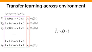
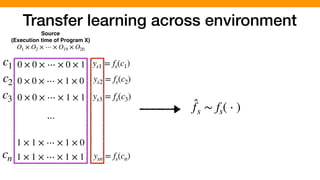
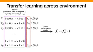
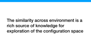
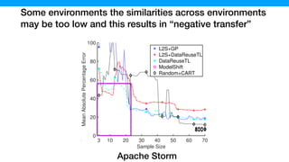
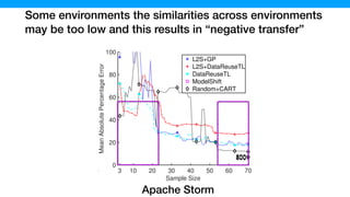
![We hypothesized that we can exploit similarities across
environments to learn “cheaper” performance models
O1 × O2 × ⋯ × O19 × O20
0 × 0 × ⋯ × 0 × 1
0 × 0 × ⋯ × 1 × 0
0 × 0 × ⋯ × 1 × 1
1 × 1 × ⋯ × 1 × 0
1 × 1 × ⋯ × 1 × 1
⋯
c1
c2
c3
cn
ys1 = fs(c1)
ys2 = fs(c2)
ys3 = fs(c3)
ysn = fs(cn)
O1 × O2 × ⋯ × O19 × O20
0 × 0 × ⋯ × 0 × 1
0 × 0 × ⋯ × 1 × 0
0 × 0 × ⋯ × 1 × 1
1 × 1 × ⋯ × 1 × 0
1 × 1 × ⋯ × 1 × 1
⋯
yt1 = ft(c1)
yt2 = ft(c2)
yt3 = ft(c3)
ytn = ft(cn)
Source Environment
(Execution time of Program X)
Target Environment
(Execution time of Program Y)
Similarity
[P. Jamshidi, et al., “Transfer learning for performance modeling of configurable systems….”, ASE’17]](https://image.slidesharecdn.com/talk-pooyan-furman2-190416181547/85/Transfer-Learning-for-Performance-Analysis-of-Machine-Learning-Systems-144-320.jpg)
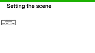
![Our empirical study: We looked at different highly-
configurable systems to gain insights
[P. Jamshidi, et al., “Transfer learning for performance modeling of configurable systems….”, ASE’17]
SPEAR (SAT Solver)
Analysis time
14 options
16,384 configurations
SAT problems
3 hardware
2 versions
X264 (video encoder)
Encoding time
16 options
4,000 configurations
Video quality/size
2 hardware
3 versions
SQLite (DB engine)
Query time
14 options
1,000 configurations
DB Queries
2 hardware
2 versions
SaC (Compiler)
Execution time
50 options
71,267 configurations
10 Demo programs](https://image.slidesharecdn.com/talk-pooyan-furman2-190416181547/85/Transfer-Learning-for-Performance-Analysis-of-Machine-Learning-Systems-145-320.jpg)


![Transfer Learning for Performance Modeling of
Configurable Systems: An Exploratory Analysis
Pooyan Jamshidi
Carnegie Mellon University, USA
Norbert Siegmund
Bauhaus-University Weimar, Germany
Miguel Velez, Christian K¨astner
Akshay Patel, Yuvraj Agarwal
Carnegie Mellon University, USA
Abstract—Modern software systems provide many configura-
tion options which significantly influence their non-functional
properties. To understand and predict the effect of configuration
options, several sampling and learning strategies have been
proposed, albeit often with significant cost to cover the highly
dimensional configuration space. Recently, transfer learning has
been applied to reduce the effort of constructing performance
models by transferring knowledge about performance behavior
across environments. While this line of research is promising to
learn more accurate models at a lower cost, it is unclear why
and when transfer learning works for performance modeling. To
shed light on when it is beneficial to apply transfer learning, we
conducted an empirical study on four popular software systems,
varying software configurations and environmental conditions,
such as hardware, workload, and software versions, to identify
the key knowledge pieces that can be exploited for transfer
learning. Our results show that in small environmental changes
(e.g., homogeneous workload change), by applying a linear
transformation to the performance model, we can understand
the performance behavior of the target environment, while for
severe environmental changes (e.g., drastic workload change) we
can transfer only knowledge that makes sampling more efficient,
e.g., by reducing the dimensionality of the configuration space.
Index Terms—Performance analysis, transfer learning.
Fig. 1: Transfer learning is a form of machine learning that takes
advantage of transferable knowledge from source to learn an accurate,
reliable, and less costly model for the target environment.
their byproducts across environments is demanded by many
Details: [ASE ’17]](https://image.slidesharecdn.com/talk-pooyan-furman2-190416181547/85/Transfer-Learning-for-Performance-Analysis-of-Machine-Learning-Systems-164-320.jpg)
![Details: [AAAI Spring Symposium ’19]](https://image.slidesharecdn.com/talk-pooyan-furman2-190416181547/85/Transfer-Learning-for-Performance-Analysis-of-Machine-Learning-Systems-165-320.jpg)

![Configurations of deep neural networks affect
accuracy and energy consumption
0 500 1000 1500 2000 2500
Energy consumption [J]
0
20
40
60
80
100
Validation(test)error
CNN on CNAE-9 Data Set
72%
22X](https://image.slidesharecdn.com/talk-pooyan-furman2-190416181547/85/Transfer-Learning-for-Performance-Analysis-of-Machine-Learning-Systems-175-320.jpg)
![Configurations of deep neural networks affect
accuracy and energy consumption
0 500 1000 1500 2000 2500
Energy consumption [J]
0
20
40
60
80
100
Validation(test)error
CNN on CNAE-9 Data Set
72%
22X
the selected cell is plugged into a large model which is trained on the combinatio
validation sub-sets, and the accuracy is reported on the CIFAR-10 test set. We not
is never used for model selection, and it is only used for final model evaluation. We
cells, learned on CIFAR-10, in a large-scale setting on the ImageNet challenge dat
sep.conv3x3/2
sep.conv3x3
sep.conv3x3/2
sep.conv3x3
sep.conv3x3
sep.conv3x3
image
conv3x3/2
conv3x3/2
sep.conv3x3/2
globalpool
linear&softmax
cell
cell
cell
cell
cell
cell
cell
Figure 2: Image classification models constructed using the cells optimized with arc
Top-left: small model used during architecture search on CIFAR-10. Top-right:
model used for learned cell evaluation. Bottom: ImageNet model used for learned
For CIFAR-10 experiments we use a model which consists of 3 ⇥ 3 convolution w](https://image.slidesharecdn.com/talk-pooyan-furman2-190416181547/85/Transfer-Learning-for-Performance-Analysis-of-Machine-Learning-Systems-176-320.jpg)
![Configurations of deep neural networks affect
accuracy and energy consumption
0 500 1000 1500 2000 2500
Energy consumption [J]
0
20
40
60
80
100
Validation(test)error
CNN on CNAE-9 Data Set
72%
22X
the selected cell is plugged into a large model which is trained on the combinatio
validation sub-sets, and the accuracy is reported on the CIFAR-10 test set. We not
is never used for model selection, and it is only used for final model evaluation. We
cells, learned on CIFAR-10, in a large-scale setting on the ImageNet challenge dat
sep.conv3x3/2
sep.conv3x3
sep.conv3x3/2
sep.conv3x3
sep.conv3x3
sep.conv3x3
image
conv3x3/2
conv3x3/2
sep.conv3x3/2
globalpool
linear&softmax
cell
cell
cell
cell
cell
cell
cell
Figure 2: Image classification models constructed using the cells optimized with arc
Top-left: small model used during architecture search on CIFAR-10. Top-right:
model used for learned cell evaluation. Bottom: ImageNet model used for learned
For CIFAR-10 experiments we use a model which consists of 3 ⇥ 3 convolution w
the selected cell is plugged into a large model which is trained on the combination of training and
validation sub-sets, and the accuracy is reported on the CIFAR-10 test set. We note that the test set
is never used for model selection, and it is only used for final model evaluation. We also evaluate the
cells, learned on CIFAR-10, in a large-scale setting on the ImageNet challenge dataset (Sect. 4.3).
sep.conv3x3/2
sep.conv3x3
sep.conv3x3/2
sep.conv3x3
sep.conv3x3
sep.conv3x3
image
conv3x3
globalpool
linear&softmax
cell
cell
cell
cell
cell
cell
Figure 2: Image classification models constructed using the cells optimized with architecture search.
Top-left: small model used during architecture search on CIFAR-10. Top-right: large CIFAR-10
model used for learned cell evaluation. Bottom: ImageNet model used for learned cell evaluation.](https://image.slidesharecdn.com/talk-pooyan-furman2-190416181547/85/Transfer-Learning-for-Performance-Analysis-of-Machine-Learning-Systems-177-320.jpg)


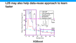


![The samples generated by L2S contains more
information… “entropy <-> information gain”
10 20 30 40 50 60 70
sample size
0
1
2
3
4
5
6
entropy[bits]
Max entropy
L2S
Random
DNN](https://image.slidesharecdn.com/talk-pooyan-furman2-190416181547/85/Transfer-Learning-for-Performance-Analysis-of-Machine-Learning-Systems-191-320.jpg)
![The samples generated by L2S contains more
information… “entropy <-> information gain”
10 20 30 40 50 60 70
sample size
0
1
2
3
4
5
6
entropy[bits]
Max entropy
L2S
Random
10 20 30 40 50 60 70
sample size
0
1
2
3
4
5
6
7
entropy[bits]
Max entropy
L2S
Random
10 20 30 40 50 60 70
sample size
0
1
2
3
4
5
6
7
entropy[bits]
Max entropy
L2S
Random
DNN XGboost Storm](https://image.slidesharecdn.com/talk-pooyan-furman2-190416181547/85/Transfer-Learning-for-Performance-Analysis-of-Machine-Learning-Systems-192-320.jpg)
![Details: [FSE ’18]](https://image.slidesharecdn.com/talk-pooyan-furman2-190416181547/85/Transfer-Learning-for-Performance-Analysis-of-Machine-Learning-Systems-194-320.jpg)


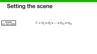
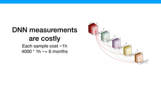
![We found many configuration with the same accuracy
while having drastically different energy demand
0 500 1000 1500 2000 2500
Energy consumption [J]
0
20
40
60
80
100
Validation(test)error
CNN on CNAE-9 Data Set
72%
22X](https://image.slidesharecdn.com/talk-pooyan-furman2-190416181547/85/Transfer-Learning-for-Performance-Analysis-of-Machine-Learning-Systems-203-320.jpg)
![We found many configuration with the same accuracy
while having drastically different energy demand
0 500 1000 1500 2000 2500
Energy consumption [J]
0
20
40
60
80
100
Validation(test)error
CNN on CNAE-9 Data Set
72%
22X
100 150 200 250 300 350 400
Energy consumption [J]
8
10
12
14
16
18
Validation(test)error
CNN on CNAE-9 Data Set
22X
10%
300J
Pareto frontier](https://image.slidesharecdn.com/talk-pooyan-furman2-190416181547/85/Transfer-Learning-for-Performance-Analysis-of-Machine-Learning-Systems-204-320.jpg)
![Details: [OpML ’19]](https://image.slidesharecdn.com/talk-pooyan-furman2-190416181547/85/Transfer-Learning-for-Performance-Analysis-of-Machine-Learning-Systems-205-320.jpg)


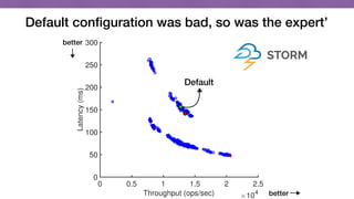
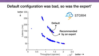
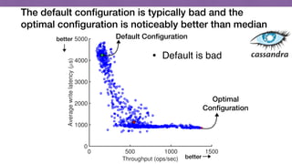
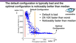
This document discusses transfer learning approaches for analyzing the performance of machine learning systems. It begins with the presenter's background and credentials. It then notes that today's most popular systems are highly configurable, but understanding how configurations impact performance is challenging. The document uses a case study of a social media analytics system called SocialSensor to illustrate the opportunity of exploring different configurations to improve performance without extra resources. Testing various configurations of SocialSensor's data processing pipelines revealed that the default was suboptimal, and an optimal configuration found through experimentation significantly outperformed the default and an expert's recommendation. The document concludes that default configurations are often bad, but transfer learning approaches can help identify configurations that noticeably improve performance.