Lecture 9h

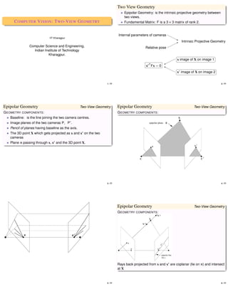
Two View Geometry
Epipolar Geometry: is the intrinsic projective geometry between
two views.
C OMPUTER V ISION : T WO -V IEW G EOMETRY Fundamental Matrix: F is a 3 × 3 matrix of rank 2.

Internal parameters of cameras �
IIT Kharagpur �
��
� Intrinsic Projective Geometry
��
Computer Science and Engineering, Relative pose �
Indian Institute of Technology
Kharagpur. � �
�� image of X on image 1 �
x
�
�
��
x� T Fx = 0 �

� �
� x� image of X on image 2

1 � 77 2 � 77

Epipolar Geometry TwoView Geometry Epipolar Geometry TwoView Geometry
G EOMETRY COMPONENTS : G EOMETRY COMPONENTS :
Baseline: is the line joining the two camera centres.
Image planes of the two cameras P� P� .
Pencil of planes having baseline as the axis.
The 3D point X which gets projected as x and x� on the two
cameras
Plane � passing through x, x� and the 3D point X.

3 � 77 4 � 77

Epipolar Geometry TwoView Geometry
G EOMETRY COMPONENTS :

Rays back projected from x and x� are coplanar �lie on �) and intersect
at X

5 � 77 6 � 77

x ↔ x� are the corresponding points.
Plane �: can be speciﬁed by the baseline and the ray
back-projected from x.
The line of intersection of � with the second image is l�
l� is the epipolar line corresponding to the point x.
The corresponding point x� lies on this epipolar line l� .

7 � 77 8 � 77

Epipole: is the point of intersection of the line joining the camera
centres �the baseline) with the image plane.
Epipole: is the image of the camera centre of the other view.
Epipolar plane: is the plane containing the baseline. There is a
one-parameter family �a pencil) of epipolar planes.
Epipolar line: is the line of intersection of the epipolar plane with
the image plane.
A LL EPIPOLAR LINES INTERSECT AT THE EPIPOLE .

9 � 77 10 � 77


11 � 77 12 � 77

Epipolar Geometry TwoView Geometry Fundamental Matrix Epipolar Geometry
G EOMETRY COMPONENTS : F UNDAMENTAL M ATRIX : F is the algebraic representation of the
epipolar geometry.
Point to line mapping: A point x has a corresponding epipolar line
l� in the second image.
x �→ l�
This mapping is the fundamental matrix F. It is a projective
mapping from points to lines.
The corresponding point x� which matches to x must lie on l� .

Motion parallel to the image plane

13 � 77 14 � 77

Fundamental Matrix Epipolar Geometry Fundamental Matrix Epipolar Geometry

G EOMETRIC D ERIVATION : G EOMETRIC D ERIVATION :
Consider a plane � not passing through either of the two camera The set of all points xi in the ﬁrst image and the corresponding
centres. points x� i in the second image are projectively equivalent, since
The ray back-projected from point x intersects plane � at point X. they are each projectively equivalent to the planar point set X.
The point X gets projected to point x� in the second image. There is a 2-D homography H� mapping each xi to x� i
The projected point x� lies on the epipolar line l� . H� is the transfer mapping from image 1 to image 2 via plane �.

15 � 77 16 � 77

Cross product matrix: e = �e1 � e2 � e3 )
� 
 0 −e3 e2 
 
[e]× =  e3 0 −e1 
 

 

 
−e2 e1 0
 

Any skew symmetric 3 × 3 matrix may be written in the form [e]×
for a suitable vector e.
Matrix [e]× is singular, and e is its null vector �right or left).
G EOMETRIC D ERIVATION :
The cross product of two 3-vectors a × b
Given the point x� the epipolar line l� passes through x� and
epipole e� a × b = [a]× b = aT [b]×
l� = [e� ]× H� x = Fx

Fundamental matrix F = [e� ]× H� Fundamental matrix F = [e� ]× H�

17 � 77 18 � 77

A LGEBRAIC D ERIVATION :
The ray back-projected from x by P is obtained by solving PX = x.
The ray is parametrized by the scalar λ.

X�λ) = P� x + λC

P� is the pseudo inverse of P, i.e. PP� = I , C is the camera
G EOMETRIC D ERIVATION : centre given by PC = 0
Fundamental matrix F = [e� ]× H� Two points on the ray are P� x �at λ = 0) and camera centre C �at
[e� ]× has rank 2, H� has rank 3, F is a matrix of rank 2. λ = ∞).
F is a mapping from IP2 onto a IP1 . These two points are imaged by the second camera P� at
F is a “point map”. It maps x �→ l� . P� x �→ P� P� x
C �→ P� C
The pencil of epipolar lines through e� forms IP1 .

19 � 77 20 � 77

A LGEBRAIC D ERIVATION : I N TERMS OF C AMERA M ATRICES :
The epipolar line joins these two projected points:
l� = �P� C) × �P� P� x) P = K[ I � 0] P� = K� [R � t]
The epipole e� = P� C, � we have l� = e� × �P� P� )x = Fx
� � � �
K−1 0
P� = C=
0� 1
F = [e� ]× P� P�

Using result:
F = [P� C]× P� P�
Comparing this with the previously derived formula F = [e� ]× H� we � �
= [K� t]× K� RK−1 [t]× M = M∗ M−1 t
have H� = P� P� . � ×
�
= K�−� [t]× RK−1 = M−� M−1 t up to scale
×
� �
= K�−� R R� t K−1 t is any vector
� × � M non-singular matrix
= K�−� RK� KR� t M∗ = det�M)M−�
×

21 � 77 22 � 77

I N TERMS OF C AMERA M ATRICES : C ORRESPONDENCE C ONDITION :
Epipoles are given by images of the camera centres: The epipolar line l� = Fx. Since point x� lies on this line, we have
x� � l� = 0. This gives x� � Fx = 0.
−R� t
� � � �
0
e=P = KR T t e� = P� = K� t The fundamental matrix satisﬁes the condition that for any
pair of corresponding points x ↔ x� in the two images
�
1 1 �

� =0�
x � � Fx
F = [P� C]× P� P� F = [P� C]× P� P�
= [K� t]× K� RK−1 F can be characterized without reference to camera matrix, only in
= [e� ]× K� RK−1 terms of �x� x� ) point correspondences.
= K�−� [t]× RK−1
� � = K�−� [t]× RK−1 F can be computed from image correspondences.
= K�−� R R� t K−1 � �
� × � = K�−� R R� t K−1 At least 7 point correspondences are required to compute F.
×
= K�−� RK� KR� t
× = K�−� RK� [e]×

23 � 77 24 � 77

P ROPERTIES : P ROPERTIES :
F is unique for two views. F has 7 degrees of freedom. A 3 × 3 homogeneous matrix has 8
F is 3 × 3 homogeneous matrix with rank 2. independent ratios. F also satisﬁes the constraint detF = 0 which
removes one degree of freedom.
If F is the fundamental matrix of the pair of cameras �P� P� ), then
F� is the fundamental matrix of the pair in opposite order �P� � P). F is a correlation: a projective map taking point to a line. l� = Fx.
Epipolar line l� = Fx contains the epipole e� . Any point x on l is mapped to the same epipolar line l� . This
means there is no inverse mapping, and F is not of full rank.
e�� Fx) = �e�� F)x = 0 for all x e�� F = 0 F is not invertible. Hence F is not a proper correlation.

Epipolar line l = F� x� contains the epipole e.

e� �F� x� ) = �e� F� )x� = 0 for all x� Fe = 0

25 � 77 26 � 77

E PIPOLAR L INE H OMOGRAPHY : E PIPOLAR L INE H OMOGRAPHY :
The set of epipolar lines in each of the images forms a pencil of The set of epipolar lines in each of the images forms a pencil of
lines passing through the epipoles. lines passing through the epipoles.
Such pencil of lines may be considered as a 1-D projective space. Such pencil of lines may be considered as a 1-D projective space.
The corresponding epipolar lines are perspectively related.
There is a homography between the pencil of lines centered at e in
the 1st view and the pencil of lines centered at e� in the 2nd view.
A homography between two such 1-D projective spaces has 3
degrees of freedom.

 2 for e�
Degrees of freedom 

 2 for e =7

for F 
 3 for epipolar line homography


27 � 77 28 � 77

E PIPOLAR L INE H OMOGRAPHY :
Suppose l and l� are corresponding epipolar lines.
Suppose k is any line passing through epipole e.

Next � �
The point of intersection of two lines l and k is x = [k]× l = k × l.
−→
This point lies on the epipolar line l.
The epipolar line corresponding to x is l� = Fx = F[k]× l What is F for special special motions between two
views.
Likewise we have l = F� x� = F� [k� ]× l� � �

29 � 77 30 � 77

S PECIAL M OTIONS BETWEEN VIEWS : S PECIAL M OTIONS BETWEEN VIEWS :
Pure translation between the two views.
Pure translation
Pure planar motion between the two views: the translation t is
orthogonal to the direction of rotation axis a The camera undergoes a translation t.
We assume there is no change in the internal parameters of the Equivalently, the camera is assumed stationary and the world
camera viewing the scene. points undergo translation −t.
Points in 3-space move on straight lines parallel to t.
On the image plane these parallel lines appear to intersect at the
vanishing point v in the direction of t.

Both the views have a common epipole v.
The imaged parallel lines are the epipolar lines.

31 � 77 32 � 77

Fundamental Matrix Epipolar Geometry
S PECIAL M OTIONS BETWEEN VIEWS :

Pure translation

Camera translating along principal axis

33 � 77 34 � 77

Fundamental Matrix Epipolar Geometry

Pure translation
The two cameras can be chosen as:

P = K[ I � 0] P� = K[ I � t]

Given that the camera coordinate system is aligned with the world
coordinate system and the camera is looking at the Z axis.

Camera translating along principal axis

35 � 77 36 � 77

Projection on the 1st camera Pure Translation
Projection on the 2nd camera Pure Translation
The inhomogeneous space point X gets projected to the � 
�inhomogeneous) image point x.  X  � 
   x 
 Y 

   
X= x� =  y  Zx� = P� X = K[ I � t] X
 
  
�     
 X   Z 
�    
 

 x  1
   
  
 Y 
    
1

X=



  y 
x=
  Zx = PX = K[ I � 0] X
 Z 
 
 




1
� 
 X 

 
  
1
   
Zx� = [K � Kt] X Zx� = K  Y  + Kt
 

 

 
Z
�   
 X 
 
ZK−1 x =  Y 
 





 Zx� = K�ZK−1 x) + Kt Zx� = Z�KK−1 x) + Kt
Z
 

x� = x + Kt/Z

The epipoles e� e� are the same in both the views and they are the
vanishing points of the imaged parallel lines in the direction t.

37 � 77 38 � 77

Pure translation Fundamental Matrix Pure translation Fundamental Matrix
The situation when S OME O BSERVATIONS :
the object translates
x� = x + Kt/Z
by −t is the same as
camera translating
by t The extent of motion depends on the magnitude of translation t
and the inverse depth Z.
The epipoles e� e� are In the case of pure translation:
the same in both the
views and they are P = K[ I � 0] P� = K[ I � t]
the vanishing points
F = [P� C]× P� P� = [e� ]× K� RK−1 = [e� ]× KK−1 = [e� ]×
of the imaged
parallel lines in the
direction t. F = [e� ]×

39 � 77 40 � 77

Pure translation Fundamental Matrix Fundamental Matrix Epipolar Geometry
S OME O BSERVATIONS : x� = x + Kt/Z F = [e� ]× S PECIAL M OTIONS BETWEEN VIEWS :
For camera translating parallel to x axis:
General Motion
�  � 
 1 
   0 0 0 
  We are given two arbitrary views:
x� Fx = 0 and thus y = y �
�  0   0 0 −1  �
e =  F=
   
 
  



 Correction 1: Rotate the camera used for the first image so that it
0 0 1 0
   
is aligned with the second camera. This rotation may be simulated
by applying a projective transformation to the first image.
The fundamental matrix has 2 dofs which correspond to the
position of the epipole. Correction 2: Apply further correction can be applied to the first
image to account for any difference in the calibration matrices
l� = Fx = [e� ]× x and x� [e� ]× x = 0. Hence x lies on line [e� ]× x = l� .
K� K� of the two cameras.
Implying that x� x� � e = e� are collinear.
This collinearity property is termed as autoepipolar and does not The result of the two corrections is a projective transformation � of
hold for general motion. the first image.
�  Now the two cameras are related by a pure translation.
 0 0 0 
 
why x � [e� ] x = 0 ? Verify: �  0 0 −1  x
x 
 
×  

 
0 1 0
 
41 � 77 42 � 77

General Motion Fundamental Matrix General Motion Fundamental Matrix
ˆ as the fundamental
After applying the two corrections we have F
matrix between the corrected ﬁrst image � and the second image,
x
i.e. �� ↔ x� �
x
ˆ
F = [e� ]× � = �x
x
�ˆ
x� F� = 0
x
�
x� [e� ]× �x = 0
Hence the fundamental matrix corresponding to the initial point
correspondences �x ↔ x� � is

F = [e� ]× �

43 � 77 44 � 77

Retrieving the camera matrices Fundamental matrix Retrieving the camera matrices Fundamental matrix
The fundamental matrix F can be used to determine the camera The fundamental matrix F only depends on the projective
matrices of the two views. properties of the cameras P� P� .
The relations l� = Fx and x� � Fx = 0 are projective relationships. F does not depend on the choice of the world coordinate frame.
They make use of the projective coordinates in the image. Rotation of world coordinates changes P� P� and not F.
Euclidean measurements such as angles are not used. If the 3-space undergoes a projective transformation �using a
If the images undergo a projective transformation, 4 × 4 H−1 )
X� = H−1 X
� = �x
x �� = H� x�
x
then the fundamental matrices corresponding to the pairs of
there is a corresponding map cameras �P� P� ) and �P�� P� �) are the same.

ˆ� = F�
l ˆx ˆ
F = H�−� FH−1 PX = �P�)�H−1 X) P� X = �P� �)�H−1 X)

x ˆx ˆ ˆ
�� F� = �H� x� )� F��x) = x� � H�� F�x = x� � Fx
� �
F = [P� C]× P� P� = P� �H−1 C �P� �)�H−1 P� )
×
�� ˆ ˆ Fundamental matrix remains unchanged.
� H F� = F hence F = H�−� FH−1

45 � 77 46 � 77

A pair of cameras can uniquely determine F. A fundamental matrix determines the two cameras at best up to a
A fundamental matrix determines the two cameras at best up to a right multiplication by a 3D projective transformation.
right multiplication by a 3D projective transformation. It will now be shown that if two pairs of camera matrices �P� P� )
˜ ˜�
and �P� P ) have the same fundamental matrix F, then the pairs of
Given two camera matrices �P� P� ), it is always possible to identify a camera matrices are related up to a right multiplication by a
homography such that �P�� P� �) will form a canonical camera pair. projective transformation �.
There always exists a non-singular 4 × 4 matrix � such that
P� = [ I � 0] P� � = [M � m]
˜ ˜�
P = P� and P = P� �.
˜ ˜�
We can assume that the two pairs of cameras �P� P� ) and �P� P ) are
The fundamental matrix corresponding to a pair of camera matrices
provided in the canonical form.
P = [ I � 0] P� = [M � m] is equal to F = [m]× M
P = [ I � 0] P� = [A � a] ˜
P = [ I � 0] ˜� ˜ a
P = [A � ˜]
Recall
F = [e� ]× P� P�

47 � 77 48 � 77

�
P = [ I � 0] �
P = [A � a] ˜
P = [ I � 0] ˜ ˜ a
P = [A � ˜] ˜
[a]× A = k [a]× A ˜
[a]× �k A − A) = 0
a ˜
F = [a]× A = [˜]× A ˜
Now, [a]× �k A − A) is a 3 × 3 matrix.
We have ˜
If we substitute �k A − A) by a 3 × 3 matrix of form av� then we ﬁnd
that [a]× av� = 0
a� F = a� [a]× A = 0 and a a a ˜
˜� F = ˜� [˜]× A = 0 ˜
Hence �k A − A) = av� where v is any 3-vector.
Since F is rank 2, it has a 1-D null space. Hence ˜ = ka
a Thus,
˜
A = k −1 �A + av� )
a ˜
Since [a]× A = [˜]× A,
˜
[a]× A = k [a]× A ˜
[a]× �k A − A) = 0

Here k is any constant.

49 � 77 50 � 77


˜
Given the two substitutions: a = k a and ˜
A=k −1
�A + av� )
P = [ I � 0] ˜
P = [ I � 0]
The camera matrices now become:
P� = [A � a] ˜�
P = [k −1 �A + av� � k a]
P = [ I � 0] ˜
P = [ I � 0]
˜�
� �
P� = [A � a] ˜ a
P = [A � ˜] k −1 I 0
We choose �=
k −1 v� k
˜
P = [ I � 0]
˜�
P = [k −1 �A + av� � k a] P = [ I � 0] ˜
P� = k −1 P
�
Is there any � which will now give P = [A � a] P� � = [A � a]�
= [k −1 �A + av� ) � ka]
˜
P� = P and ˜�
P� � = P ˜ a ˜�
= [A � ˜] = P
˜ ˜�
Thus we have P� = P and P� � = P

51 � 77 52 � 77

Degrees of Freedom Fundamental matrix Computing camera matrices Fundamental matrix
Each of the two camera matrices �P� P� ) have 11 degrees of F can determine the camera pair up to a projective transformation
freedom. Total: 22 dofs. of 3-space.
Specifying a projective world frame requires 15 dofs. If any matrix, say M is skew symmetric, we have x� Mx = 0
22-15 = 7. Consider the composite matrix P�� FP
The fundamental matrix F has 7 degrees of freedom.
X� P�� FPX = 0
�
we have since x� Fx = 0

A non-zero matrix F is the fundamental matrix corresponding to a
pair of camera matrices P and P� if and only if P�� FP is skew
symmetric.

53 � 77 54 � 77

Computing camera matrices Fundamental matrix Computing camera matrices Fundamental matrix
Consider F to be the given Fundamental matrix.
Consider a pair of 3 × 4 matrices Check P�� FP is skew symmetric
�
� � � � � � � �
P = [ I � 0] P� = [SF � e� ] such that e� F = 0 [SF � e� ]� F [ I � 0] =
F S F 0
=
F S F 0
e�� F 0 0� 0
Assume that P� P� have rank 3.
This is indeed skew symmetric if S is skew symmetric.
We need to verify if P� P� are indeed the camera matrices
corresponding to F. Following conditions need to be checked:
Choosing a suitable matrix S
S is skew symmetric. In terms of its null vector S = [s]× .
We need to verify that P�� FP is skew symmetric.
We need to choose a skew symmetric matrix S such that P� has P� = [SF � e� ] = [ [s]× F � e� ]
rank 3.

55 � 77 56 � 77


� �
Choosing a suitable matrix S Choosing a suitable matrix S

� �
Choose S = [s]× . [ [s]× F � e� ] will have rank 3 provided s� e� � 0.
� � �
P = [SF � e ] = [ [s]× F � e ]
[s]× F has rank 2. The column space of [s]× F is spanned by the
� �
We need to verify that P� = [ [s]× F � e� ] has rank 3. cross product of s with the columns of F, and � equals the plane
perpendicular to s.
� �
[ [s]× F � e� ] will have rank 3 provided s� e� � 0. Why?
If s� e� � 0 then e� is not perpendicular to s, and hence it does not
lie in this plane.
Thus [ [s]× F � e� ] has rank 3.

A suitable choice for s can be e� since we have e� � e� � 0.
Thus we take S = [s]× = [e� ]×

57 � 77 58 � 77

The camera matrices corresponding to the Fundamental matrix F FAMILY OF CAMERAS WHICH HAVE THE SAME F

� �
can be chosen as:
�
P = [ I � 0] P� = [[e� ]× F � e� ] such that e� F = 0
We can identify a family of cameras:
The left 3 × 3 sub-matrix of i.e. P� [e� ]
× F has rank 2. This
corresponds to a camera with centre at �∞ . P = [ I � 0] P� = [[e� ]× F � e� v� � k e� ]

v�k are parameters
� �
v is any 3-vector and k is a non-zero scalar.

59 � 77 60 � 77

Fundamental matrix Essential Matrix A special case of F
The Essential matrix is a special case of fundamental matrix for a
pair of normalized cameras.
It has fewer degrees of freedom and additional properties.

Next � �
It makes use of normalized image coordinates.
−→

After Fundamental matrix: ..... Normalized Coordinates

The Essential Matrix P = K[R � t] x = PX � = K−1 x = [R � t]X
x
� �
The matrix K−1 P = [R � t] is the normalized camera matrix.
We have the normalized camera pair: P = [ I � 0] and P� = [R � t]

61 � 77 62 � 77

Essential Matrix A special case of F Essential Matrix A special case of F
−1 ��
P = K[R � t] x = PX � = K x = [R � t]X
x � E� = 0
x x

The Fundamental matrix corresponding to the normalized camera Substituting for � = K−1 x and �� = K−1 x� gives
x x
pair P = [ I � 0] and P� = [R � t] is called as the Essential matrix:
x� K�−� EK−1 x = 0 F = K�−� EK−1 E = K�� FK
�
� �
E = [t]× R = R R� t
×
Properties of Essential Matrix
We have
��
� E� = 0
x x Has 5 dofs: 3 for R and 3 for t and -1 for overall scale.
A 3 × 3 matrix is an essential matrix if and only if two of its
For the corresponding points x ↔ x� , the normalized image singular values are equal and third is zero.
coordinates are � ↔ ��
x x

63 � 77 64 � 77

Consider decomposition of E as

E = SR = [t]× R

Next � �
S is a skew-symmetric matrix which can be decomposed as
−→
S = k UZU� where U is orthogonal
We show that E has TWO singular values which
are equal and the third is zero
� �
Matrix Z is a block diagonal matrix of the form
�  � � 
 0 1 0 
   1 0 0   0 −1 0 
  
Z=  −1 0 0  as a matrix product =  0 1 0   1 0 0 
 
 
 
 


 
 
 
 

0 0 0 0 0 0 0 0 1
    

65 � 77 66 � 77

Consider decomposition of E as Consider decomposition of E as �up to scale)

E = SR = k UZU� R = [t]× R E = SR = UZU� R = [t]× R

Z is skew symmetric and SVD decomposition of

E = UDV� = U diag�1,1,0) �WU� R) where V� = �WU� R)
� 
 0 −1 0 
 
Z = diag�1,1,0) W where  1 0 0 
W=
 


 

0 0 1
 
Thus E has two singular values which are equal.
W turns out to be an orthogonal matrix. S = UZU � SVD of E is not unique. Alternate SVDs are given as:

S = U diag�1,1,0) W U� � E = SR = U diag�1,1,0) �WU� R) E = �Udiag�R2×2 � 1)) diag�1,1,0) �diag�R� � 1)V� )
2×2

where R2×2 is any rotation matrix.

67 � 77 68 � 77

Essential Matrix A special case of F Extraction of Cameras Essential matrix E
Consider decomposition of E as �up to scale)

E = SR = [t]× R

P� = [R � t]
Next � �
The two cameras can be chosen as: P = [ I � 0]
−→
The vector t has to be chosen such that St = 0.
How to extract cameras from E SVD of E is not unique. Alternate SVDs are given as:
� �
E = UDV� = U diag�1,1,0) �WU� R) where V� = �WU� R)
� 
 0
 −1 0 
W= 1 0 0 
 

 

 
0 0 1
 

R = UW� V�

69 � 77 70 � 77

Extraction of Cameras Essential matrix E Extraction of Cameras Essential matrix E
Consider decomposition of E as It can be veriﬁed that St = 0

E = SR = [t]× R St = �U diag�1,1,0) W U� ) t
= �U diag�1,1,0) W U� ) u�
The two cameras can be chosen as: P = [ I � 0] P� = [R � t]
� � � � � 
The vector t has to be chosen such that St = 0.  a1
 a2 a3   1 0 0   0 −1 0   a1
   b1 c1   a3 
 
 b

 1  0 1 0  1 0 0  a
b2 b3  
 
 
 2 b2 c2   3 
 b 


We choose

 
 
 
 
 

c1 c2 c3 0 0 0 0 0 1 a3 b3 c3 c3
     
t = U�0� 0� 1)� = u� � �  � � 
 a1 a2 a3   0 −1 0   a1 b1 c1   a3 
It can be veriﬁed that St = 0 
 b

 1

b2 b3   1 0 0 






 a

 2




b2 c2   b3 



 
 
 
 
 

St = �U diag�1,1,0) W U� ) t c1 c2 c3 0 0 0 a3 b3 c3 c3
     

= �U diag�1,1,0) W U� ) u�
�  � � 
 a2
 −a1 0   a1
 b1 c1   a3 
 
 b

−b1 0 
  a

b2 c2   3 
 b 
 
=0  2





 2

 
 

c2 −c1 0 a3 b3 c3 c3
    

71 � 77 72 � 77

Extraction of Cameras Essential matrix E Extraction of Cameras Essential matrix E
Consider decomposition of E as
�  � 
 a2 a1 − a1 a2 a2 b1 − a1 b2 a2 c1 − a1 c2 
   a3 
 
 b a −b a b b −b b b c −b c 

 2 1
  b 

 3 
1 2 2 1 1 2 2 1 1 2  
E = SR = [t]× R

 
 
 

c2 a1 − a2 c1 c2 b1 − c1 b2 c2 c1 − c1 c2 c3
   

The two cameras can be chosen as: P = [ I � 0] P� = [R � t]
�  � 

 0 a2 b1 − a1 b2 a2 c1 − a1 c2    a3 
 
 b2 a1 − b1 a2 0 b2 c1 − b1 c2   b 

  
 
  3 
 
 We choose
   
c2 a1 − a2 c1 c2 b1 − c1 b2 0 c3
   
�  t = U�0� 0� 1)� = u� R = UW� V�
 a2 b1 b3 − a1 b2 b3 + a2 c1 c3 − a1 c2 c3 
 
 a b a −a b a +b c c −b c c 

 3 2 1 
3 1 2 2 1 3 1 3 2 

 
 There are 4 possible pairs of cameras:
c2 a3 a1 − a2 a3 c1 + c2 b1 b3 − c1 b2 b3
 
�

 �
a2 �b1 b3 + c1 c3 ) − a1 �b2 b3 + c2 c3 )   a2 a1 a3 − a1 a2 a3 
 P� = [R � t] P� = [R � t]
� �
= [UWV� � + u� ]
   
b2 �a3 a1 + c1 c3 ) − b1 �a3 a2 + c3 c2 )  =  b2 b1 b3 − b1 b2 b3  = 0 = [UW V � + u� ]

  
  


   
   
c2 �a3 a1 + b1 b3 ) − c1 �a2 a3 + b2 b3 ) c2 c1 c3 − c1 c2 c3 = [UW� V� � − u� ] = [UWV� � − u� ]
   

73 � 77 74 � 77

Extraction of Cameras Essential matrix E
There are 4 possible pairs of cameras:

P� = [R � t] P� = [R � t]
= [UW� V� � + u� ] = [UWV� � + u� ]
� �
= [UW V � − u� ] = [UWV� � − u� ]

W and W� are related by a rotation througth 1800 about the
base-line.

75 � 77 76 � 77

Summary
Intrinsic projective geometry of 2-views.
Epipolar geometry
Fundamental matrix
Deriving the fundamental matrix from camera matrices.
Deriving the fundamental matrix from point correspondences.
Deriving the camera matrices from the fundamental matrix.
Essential matrix
Deriving the camera matrices from the essential matrix.

77 � 77

Lecture 9h

Recommended

Recommended

More Related Content

What's hot

What's hot (20)

Viewers also liked

Viewers also liked (7)

Similar to Lecture 9h

Similar to Lecture 9h (9)

More from Krishna Karri

More from Krishna Karri (17)

Lecture 9h