HOMEWORK SOLUTION PROBLEMS ON WATER TREATMENT OPERATION PARAMETERS

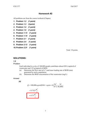
1. CEE 577 Fall 2017
1
Homework #2
All problems are from the course textbook (Chapra).
1. Problem 1.2 (1 point)
2. Problem 1.3 (1point)
3. Problem 1.4 (1 point)
4. Problem 1.6 (1 point)
5. Problem 1.13 (1 point)
6. Problem 1.14 (1 point)
7. Problem 2.1 (1 point)
8. Problem 2.4 (1 point)
9. Problem 2.13 (1 point)
10.Problem 2.21 (1 point)
Total: 10 points
SOLUTIONS:
1.2
Problem
Each individual in a city of 100,000 people contributes about 650 L/capita/d of
wastewater and 135 g/capita/d of BOD.
(a) Determine the flow rate (m3
s-1
) and mass loading rate of BOD (mta)
generated by such a population.
(b) Determine the BOD concentration of the wastewater (mg/L)
Answer
(a)
( )
s
m
s
m
s
d
L
m
d
capita
L
capita
Q
3
3
3
3
75
.
0
7523
.
0
400
,
86
1
10
1
/
/
650
000
,
100
≈
=
=

2. CEE 577 Fall 2017
2
( )
mta
x
mta
kg
mta
g
kg
yr
d
d
capita
g
capita
W
3
3
3
10
9
.
4
5
.
4927
10
1
10
1
365
/
/
135
000
,
100
≈
=
=
(b)
L
mg
L
mg
or
m
g
m
L
d
capita
L
d
capita
g
Q
W
c
/
208
7
.
207
1
10
/
/
650
/
/
135
3
3
3
≈
=
=
=
1.3
Problem
You are studying a 3-km stretch of stream that is about 35 m wide. A gaging
station on the stream provides you with an estimate that the average flow rate
during your study was 3 cubic meters per second (cms). You toss a float into the
stream and observe that it takes about 2 hr to traverse the stretch. Calculate the
average velocity (mps), cross-sectional area (m2
), and depth (m), for the stretch.
To make these estimates, assume that the stretch can be idealized as a rectangular
channel (constant L, B & H).
Answer
s
m
s
m
hr
km
t
L
U s
hr
km
m
4
.
0
4167
.
0
2
3
3600
1
1000
≈
=
=
=
2
2
.
7
4167
.
0
3
m
mps
cms
U
Q
A
=
=
=
m
m
m
m
B
A
H
21
.
0
206
.
0
35
2
.
7 2
≈
=
=
=

3. CEE 577 Fall 2017
3
1.4
Problem
In the early 1970s Lake Michigan had a total phosphorus loading of 6950 mta
and an in-lake concentration of 8 ug/L (Chapran and Sonzogni 1979).
(a) Determine the lake’s assimilation factor (km3
yr-1
).
(b) What loading rate would be required to bring in-lake levels down to
approximately 5 ug/L?
(c) Express the results of(b) as a percent reduction.
Answer
(a)
yr
km
x
yr
km
m
mg
mta
c
W
a m
km
tonne
mg
3
2
3
10
10
3
10
7
.
8
75
.
868
8
6950
3
9
3
9
≈
=
=
=
(b)
mta
x
mta
L
g
L
g
mta
ac
W
3
10
3
.
4
5
.
4343
/
5
/
75
.
868
≈
=
=
= µ
µ
(c)
( )
%
5
.
37
%
100
6950
75
.
4343
6950
%
100
%
=
−
=
−
=
present
future
present
W
W
W
reduction
1.6
Problem
You mix two volumes of water having the following characteristics:
Volume 1 Volume 2
Volume 1 gal 2 L
Concentration 250 ppb 2000 mg/m3
a. Calculate the concentration (mg/L) for the mixture
b. Determine the mass in each volume and in the final mixture. Express your result in
grams.

4. CEE 577 Fall 2017
4
Answer
(a)
L
gal
L
gal
V 7854
.
3
264172
.
0
1
1
1 =
=
( ) ( )
L
mg
L
mg
L
L
L
mg
L
L
mg
L
V
V
c
V
c
V
c
86
.
0
855
.
0
2
7854
.
3
/
2
2
/
250
.
0
7854
.
3
2
1
2
2
1
1
≈
=
+
+
=
+
+
=
(b)
( ) g
x
g
x
L
L
mg
V
c
m mg
g 3
3
10
1
1
1 10
95
.
0
10
9464
.
0
7854
.
3
250
.
0 3
−
−
≈
=
=
=
( ) g
x
L
L
mg
V
c
m mg
g 3
10
2
2
2 10
4
2
2 3
−
=
=
=
( ) g
x
g
x
L
L
mg
cV
m mg
g 3
3
10
10
9
.
4
10
9464
.
4
7854
.
5
855
.
0 3
−
−
≈
=
=
=
1.13
Problem
The Boulder, Colorado, wastewater treatment plant enters Boulder Creek just above a
USGS flow gaging station.
USGS
Station
WWTP
550 m
Boulder
Creek
At 8:00 A.M. on December 29, 1994, conductivities of 170, 820, and 639 µmho/cm were
measured at A, B and C respectively. (Note: Conductivity provides an estimate of the
total dissolved solids (TDS) in a solution by measuring its capability to carry an electrical
current.) If the flow at the gaging station was 0.494 cms, estimate the flows for the
treatment plant and the creek.
Answer
The flow in the creek and the treatment plant should be equal to the flow below the
mixing point,
494
.
0
=
+ B
A Q
Q

5. CEE 577 Fall 2017
5
Because conductivity and TDS are conservative substances, the following mass balance
should hold
( )
494
.
0
)
820
(
170
639 B
A Q
Q +
=
These two equations can be combined to yield,
( ) ( )
494
.
0
)
820
(
494
.
0
170
639 A
A Q
Q −
+
=
which can be solved for:
( ) cms
cms
QA 138
.
0
13756
.
0
820
170
820
639
494
.
0
≈
=
−
−
= The Creek
cms
QB 356
.
0
13756
.
0
494
.
0 =
− The Treatment Plant
1.14
Problem
Sediment traps are small collecting devices that are suspended in the water column to
measure the downward flux of settling solids. Suppose that you suspend a rectangular
trap (1m x 1m) at the bottom of a layer of water. After 10 d, you remove the trap and
determine that 20 g of organic carbon has collected on its surface.
(a) Determine the downward flux of organic carbon
(b) If the concentration of organic carbon in the water layer is 1 mg/L, determine the
downward velocity of organic carbon
(c) If the surface area at the bottom of the layer is 105
m2
, calculate how many
kilograms of carbon are transported across the area over a 1-month period.
Answer
(a)
d
m
g
d
m
g
J 2
2
2
)
10
(
1
20
=
=
(b)
d
m
m
g
d
m
g
c
J
v 2
/
1
/
/
2
3
2
=
=
=
(c)
( ) kg
kg
g
kg
month
d
m
month
d
m
g
M 100
,
6
084
,
6
10
42
.
30
10
1
2 3
2
5
2
≈
=
=
2.1
Problem
You perform a series of batch experiments and come up with the following data:
t (hr) 0 2 4 6 8 10

6. CEE 577 Fall 2017
6
C (µg/L) 10.5 5.1 3.1 2.8 2.2 1.9
Determine the order (n) and the rate constant (k) for the underlying reaction.
Solution
Consider both integral and differential approaches. The following table includes
calculations for both.
t (hr) C
(ug/L)
lnC 1/C 1/(C^2) dc/dt t-
midpoint
C-
midpoint
∆C/∆t
0 10.5 2.351375 0.095238 0.00907 4 1 7.8 2.7
2 5.1 1.629241 0.196078 0.038447 1.7 3 4.1 1
4 3.1 1.131402 0.322581 0.104058 0.5 5 2.95 0.15
6 2.8 1.029619 0.357143 0.127551 0.27 7 2.5 0.3
8 2.2 0.788457 0.454545 0.206612 0.12 9 2.05 0.15
10 1.9 0.641854 0.526316 0.277008 0.08
Prepare integral plots for 1st
, 2nd
, and 3rd
order reactions:
y = -0.1596x + 2.06
R² = 0.8908
0
0.5
1
1.5
2
2.5
0 2 4 6 8 10 12
LnC
Time (hr)
First Order Kinetics

7. CEE 577 Fall 2017
7
Of the three integral plots, the one presuming second order appears to fit slightly better
than the third order plot. You could end the problem here.
Or you could continue testing via a more “advanced” differential approach. The first, I
will call “direct differential”. This comes directly from the midpoint slopes (∆C/∆t) and
the midpoint concentrations. A log-log plot gives a slope indicative of the reaction order,
and an intercept which yields the reaction rate.
y = 0.0424x + 0.1135
R² = 0.9832
0
0.1
0.2
0.3
0.4
0.5
0.6
0 2 4 6 8 10 12
1/C
Time (hr)
Second Order Kinetics
y = 0.0267x - 0.0063
R² = 0.9749
-0.05
0
0.05
0.1
0.15
0.2
0.25
0.3
0 2 4 6 8 10 12
1/C^2
Time (hr)
Third Order Kinetics

8. CEE 577 Fall 2017
8
A second differential method involves some graphical smoothing. Refer to Chapra’s
example 2.2 on page 33 for a description as to how this can be done. The graph below
presents the results of this analysis.
One last approach is the use of non-linear least squares analysis. This is a powerful
technique that is now easily done with modern numerical software. Many statistical
packages have routines that will do this.
Integral Direct
Differential
Smoothed
Differential
Non-linear
Least Squares
Order 2 2.26 2.33 2.23
Rate constant 0.0424 0.0274 0.0239 0.0326
y = 2.2605x - 1.5615
R² = 0.8702
-1
-0.8
-0.6
-0.4
-0.2
0
0.2
0.4
0.6
0 0.2 0.4 0.6 0.8 1
log(dc/dt)
Log (t)
Direct Differential
y = 2.3334x - 1.6213
R² = 0.9441
-1.5
-1
-0.5
0
0.5
1
0 0.2 0.4 0.6 0.8 1 1.2
Log
(dc/dt)
Log (t)
Smoothed Differential

9. CEE 577 Fall 2017
9
Units on the various rates constants are “hr-1
(µg/L)n-1
”.
2.4
Problem
At a later date the laboratory informs you that they have a more complete data set than
the two measurements used in Example 2.5:
T ( C) 4 8 12 16 20 24 28
k (d-1
) 0.120 0.135 0.170 0.200 0.250 0.310 0.360
Use this data to estimate θ and k at 20 C/
Solution
Taking the logarithm of equation 2.44 yields:
θ
log
)
20
(
))
20
(
log(
))
(
log( −
+
= T
k
t
k
Thus, a plot of Log[k(t)] versus (T-20) should yield a straight line with a slope of logθ
and an intercept of log[k(20]. Linear regression can be used to do this yielding:
)
20
(
020722
.
0
60474
.
0
))
(
log( −
+
−
= T
t
k
049
.
1
0489
.
1
10 020722
.
0
≈
=
=
θ
1
60474
.
0
20 248
.
0
10 −
−
=
= d
k
2.13
Problem
Estimate the age of the fossil remains of a skeleton with 2.5% or its original carbon-14
content. Note that carbon-14 has a half-life of 5730yr.
Solution
The first-order decay model can be expressed in terms of half-life as:
2
/
1
693
.
0
t
t
oe
c
c
−
=
which can be solved for:
yrs
c
c
t
t o
500
,
30
025
.
0
1
ln
693
.
0
5730
ln
693
.
0
2
/
1
=






=






=
2.21
Problem
A more complete representation (as compared to equation 2.3) of the decomposition
reaction in provided by:
C106H263O110N16P1 + 107O2 + 14H+
→ 106CO2 + 16NH4
+
+ HPO4
-2
+ 108H2O

10. CEE 577 Fall 2017
10
On the basis of this equation, given that 10 g-C m-3
of organic matter is decomposed,
calculate (a) the stoichiometric ratio for the amount of oxygen consumed per carbon
decomposed, roc, (b) the amount of oxygen consumed in g-O/m3
, and (c) the amount of
ammonium released in mg-N/m3
.
Solution
(a)
C
g
O
g
x
x
roc
−
−
=
= 69
.
2
12
106
32
107
(b)
3
3
9
.
26
69
.
2
10
m
O
g
C
g
O
g
x
m
C
g −
=
−
−
−
(c)
3
3
3
1761
10
12
106
14
16
10
m
N
mg
N
g
N
mg
C
g
x
N
g
x
x
m
C
g −
=
−
−
−
−
−