Risks 09-00074-v2

1. risks
Article
Bitcoin and Altcoins Price Dependency: Resilience and
Portfolio Allocation in COVID-19 Outbreak
Ahmet Faruk Aysan 1,* , Asad Ul Islam Khan 2 and Humeyra Topuz 3
Citation: Aysan, Ahmet Faruk, Asad
Ul Islam Khan, and Humeyra Topuz.
2021. Bitcoin and Altcoins Price
Dependency: Resilience and Portfolio
Allocation in COVID-19 Outbreak.
Risks 9: 74. https://doi.org/10.3390/
risks9040074
Academic Editor: Pawel Smaga
Received: 18 March 2021
Accepted: 6 April 2021
Published: 13 April 2021
Publisher’s Note: MDPI stays neutral
with regard to jurisdictional claims in
published maps and institutional affil-
iations.
Copyright: © 2021 by the authors.
Licensee MDPI, Basel, Switzerland.
This article is an open access article
distributed under the terms and
conditions of the Creative Commons
Attribution (CC BY) license (https://
creativecommons.org/licenses/by/
4.0/).
1 Islamic Finance and Economy Program, College of Islamic Studies, Hamad Bin Khalifa University,
34110 Doha, Qatar
2 Department of Economics, School of Humanities and Social Sciences, Ibn Haldun University,
34480 Istanbul, Turkey; asad.khan@ihu.edu.tr
3 Department of Business Administration, Universidad Carlos III de Madrid, 28001 Madrid, Spain;
htopuz@emp.uc3m.es
* Correspondence: aaysan@hbku.edu.qa
Abstract: The main aim of this article is to examine the inter-relationships among the top cryptocur-
rencies on the crypto stock market in the presence and absence of the COVID-19 pandemic. The nine
chosen cryptocurrencies are Bitcoin, Ethereum, Ripple, Litecoin, Eos, BitcoinCash, Binance, Stellar,
and Tron and their daily closing price data are captured from coinmarketcap over the period from
13 September 2017 to 21 September 2020. All of the cryptocurrencies are integrated of order 1 i.e.,
I(1). There is strong evidence of a long-run relationship between Bitcoin and altcoins irrespective of
whether it is pre-pandemic or pandemic period. It has also been found that these cryptocurrencies’
prices and their inter-relationship are resilient to the pandemic. It is recommended that when the
investors create investment plans and strategies they may highly consider Bitcoin and altcoins jointly
as they give sustainability and resilience in the long run against the geopolitical risks and even in the
tough time of the COVID-19 pandemic.
Keywords: bitcoin; altcoins; cointegration; price dependency; COVID-19
JEL Classification: C30; E58; G28; O35
1. Introduction
Bitcoin is known to be the first distributed cryptocurrency in the foremost tech-
nology of blockchain system, which was instigated by Satoshi Nakamoto in 2008. Be-
cause of this invention, more than two thousand cryptocurrencies adhere to Bitcoin.
These currencies are known as altcoins, which are traded non-stop, 24/7 in the crypto
stock markets (CoinMarketCap 2019). Each of them has its own story which includes
its mission, vision, and values. For instance, Ethereum is a global, open-source plat-
form from which investors can run their smart contracts for decentralized applications,
(Ethereum White Paper 2019). As another example, even though Ripple’s system is based
on a central structure, Ripple aims to create a network among the international financial in-
stitutions to decrease their transaction costs and to facilitate faster global payments. Unlike
many other alt currencies, Ripple is working with governments and central financial insti-
tutions (Ripple White Paper 2019). On the contrary, Binance was initiated to be an altcoin
to create an independent ecosystem by freeing users from central organizations and gov-
ernment regulations. In addition, on the infrastructure of Tron (TRX)’s system, investors or
users can freely create, publish, and store their data sets. By using this feature of blockchain
infrastructure, Tron strives to create a global entertainment platform for content creators
and consumers in the blockchain-based decentralized platform, (Tron White Paper 2019).
After Bitcoin, these attempts of altcoins have brought about a sudden rise in the market size
of cryptocurrencies. Whilst many altcoins emerged after Nakamoto’s initiative. Bitcoin,
Risks 2021, 9, 74. https://doi.org/10.3390/risks9040074 https://www.mdpi.com/journal/risks

2. Risks 2021, 9, 74 2 of 13
Ethereum, Ripple, Litecoin, Eos, BitcoinCash, Binance, Stellar, and Tron have been ranked
among the top 20 cryptocurrencies over time by market capitalization and considered
mainstream coins (CoinMarketCap 2019).
Especially after a sudden price increase of Bitcoin in 2017, people showed a great
interest which has led to the rapid growth of cryptocurrencies. These attempts triggered
scholars, crowdfunding managers, investors, and crypto portfolio managers to assess the
long and short-term relationship among cryptocurrencies in the crypto stock market. A
lot of studies were carried out to investigate about the price bubbles in cryptocurrencies
in general especially Bitcoin, trading strategies and opportunities, financial bubbles being
created by the crypto market, the spillovers between different crypto markets, and many
more. Some of these studies are (Giudici and Pagnottoni 2019; Agosto and Cafferata 2020;
Resta et al. 2020; J McNeil 2021) and many more. In addition, highly volatile cryptocur-
rencies have high correlations. Therefore, the number of research papers has increased
to figure out long-term co-movements of prices of different cryptocurrencies and mean-
reverting strategies which analyze whether prices revert to the average or mean price,
(Leung and Nguyen 2019). To construct meaningful and stable models, researchers use
various variables and prediction techniques. (Chuen et al. 2017), for example, examined
the possibility of diversification of cryptocurrency portfolio for investors as a new invest-
ment opportunity based upon historical price and trading volume of a cryptocurrency.
Accordingly, they found out that there is a low corrselation between cryptocurrencies and
traditional investments. Another result showed that most cryptocurrencies have higher
daily returns than traditional assets.
Another strand of literature is about the possibility of cointegrating relationships
among cryptocurrencies, which makes scholars keen to search for cointegration studies.
Leung and Nguyen (2019) focused on the process of constructing cointegrated portfolios
of cryptocurrencies by employing Johansen and Engle–Granger cointegration tests. In
addition to that Bação et al. (2018) observed that a robust relationship exists between
information transmission and Bitcoin, Litecoin, Ripple, Ethereum, and Bitcoin Cash prices
by using the Vector Auto-Regression (VAR) modeling approach from 1 May 2013 to 14
March 2018. Their results suggest that Bitcoin has the power to dominate others regard-
ing information transmission due to its paramount capacity of trading volume, market
capitalization, and exchange trading volume. On the other hand, they found some counter-
arguments against their hypothesis. Some delayed information takes place, especially from
Litecoin to Bitcoin. Furthermore, the main aim of Ciaian and Rajcaniova (2018) empirical
investigation was to assess the virtual relationships between Bitcoin and altcoins in the
short and long run. Their empirical results conclude that Bitcoin and altcoin markets are
interdependent based on daily data from 2013 to 2016. Their findings confirm that in the
long run, macroeconomic indicators have an impact on price creation to a certain degree.
Therefore, exogenous factors might be recognized as determinants to a certain extent for
the crypto market. Furthermore, the ARDL technique was used by Sovbetov (2018), to
reveal that the attractiveness of cryptocurrencies plays an important role in price formation
solely in the long run. On the other hand, market beta, trading volume, and volatility
(crypto market-related factors) matter for both long- and short-term price determination
based on evidence from Bitcoin, Ethereum, Dash, Litecoin, and Monero over 2010–2018,
using weekly data. Nicaise et al. (2019) examined the co-movements in market quality of
cryptocurrencies by using intraday data of the transactions and order book of the cryp-
tocurrencies which have the highest market capitalization from August 2017 to July 2018.
Finally, Joline (2019) organized his analysis according to Engle-Granger two-step approach,
Johansen Cointegration test, and Vector Error Correction Model (VECM) to demonstrate
cointegration between Bitcoin and other altcoins; Ethereum, Ripple, Bitcoin Cash, EOS, and
Litecoin based upon daily prices in five different periods that due is 9 April 2019. Findings
prove that Bitcoin has cointegration with Ripple, Litecoin, Bitcoin Cash, and Ethereum,
albeit not with EOS. Hence, he concluded that Bitcoin is statistically crucial for the price
formation of Ripple, Litecoin, Bitcoin Cash, and Ethereum, but not EOS.

3. Risks 2021, 9, 74 3 of 13
Overall, this paper highlights the need for new analysis to examine price dependency
and long and short-term cointegration among all cryptocurrencies regarding different
periods, as this crypto market continues to develop with its new coins, along with its
new applications, regulations, and attractive narratives. More specifically the long-run
relationship among Bitcoin and altcoins has not been assessed in presence of the current
pandemic (COVID-19). Our paper contributes to this gap. Furthermore, the resilience
of this long run relationship has not been tested in the literature. This paper is aimed to
address these two issues.
Our results reveals that some cryptocurrencies have a closer relationship concerning
their price dependencies as time goes by in the COVID-19 pandemic. It offers investors to
allocate their portfolios to balance their risks in the pandemic. Furthermore, even though
each cryptocurrency has different narratives, aims, and functions, there is no one winner
on the stock market or our result does not demonstrate the zero-sum game. Our research
also provides objectively and reasonably adaptable analysis, especially for beginner crypto
enthusiasts and investors.
Our results also shows that when investors design their portfolio, they can make
diversification among these top cryptocurrencies. The paper offers investors a more diver-
sified and balanced portfolio for the long term. Overall, this article would be beneficial
for investors who would like to diversify their portfolios for the long term. Preparing a
long-term portfolio would be more strategic because of the “novel features of the market”
as Shams (2019) defined in his paper. More broadly, far from being static and narrow-
minded, the market is ever-changing dynamically; it permits investors, portfolio managers,
and policymakers to design or manage their portfolios. Finally, when investors create
investment strategies, focusing on altcoins together with Bitcoin can provide sustainabil-
ity and resilience for the long term against the geopolitical risks due to the tendency of
the long-term relationship between Bitcoin and other altcoins even in the tough periods
of the COVID-19 pandemic. Since every investor’s optimization relies on different pa-
rameter it is difficult to give exact calculations how their portfolio will be optimized by
focusing on altcoins. Moreover, at least our results shows that there is scope for such an
improvement. Portfolio optimization with altcoins could be a follow up work of this paper.
However, we confidently assert that our conclusion matches partially with the conclusions
of (Huang et al. 2021; Umar et al. 2021; Zhang and Wang 2021; Mariana et al. 2021).
Hence, this paper is designed as follows. Section 2 explains data and methodology. In
Section 3, empirical findings and results are presented based on the Johansen Cointegration
model as well as Vector Error Correction (VECM). The last section concludes.
2. Data Collection and Methodology
We use daily prices of cryptocurrencies and our data sets were obtained from the
coinsmarket.cap (2020) from 13 September 2017 to 21 September 2020. The abbreviations
used in this study with their complete description are listed in Table 1.
Table 1. Abbreviations Used In The Study.
Abbreviation Full Description
BT ln (Bitcoin closing price)
BC ln (BitcoinCash closing price)
ET ln (Ethereum closing price)
BN ln (Binance closing price)
LT ln (Litecoin closing price)
RP ln (Ripple closing price)
TR ln (Tron closing price)
ST ln (Stellar closing price)

4. Risks 2021, 9, 74 4 of 13
Table 1. Cont.
Abbreviation Full Description
EO ln (Eos closing price)
DP
DP = 1 if t ≥ 11 − 03 − 2020
DP = 0 elsewhere ∀ t = 09 − 13 − 2017 to 09 − 21 − 2020
Before we employ unit root tests and the Johansen cointegration technique, we make
general observations of descriptive statistics. In Table 2, there is a summary of descriptive
statistics for the chosen 9 cryptocurrency prices.
Table 2. Descriptive Statistics.
Crypto Currencies BC BN BT EO ET LT RP ST TR
Mean 5.979050 2.489788 8.923931 1.382447 5.569162 4.234047 −1.064664 −2.219531 −3.900057
Median 5.773277 2.678965 8.982603 1.327075 5.434246 4.090002 −1.186821 −2.303816 −3.809241
Maximum 8.274630 3.658936 9.878036 3.069912 7.241667 5.881482 1.217876 −0.109562 −1.511608
Minimum 4.348599 −0.387452 8.056728 −0.706790 4.434500 3.155297 −1.968723 −4.546901 −6.552181
Std. Dev. 0.753795 0.780537 0.362569 0.678709 0.590756 0.529539 0.536189 0.789454 0.800641
Skewness 0.658173 −1.597372 −0.442579 −0.488491 0.660800 0.767978 1.285009 −0.065045 −1.126748
Kurtosis 2.842304 5.553269 2.826004 4.129425 2.729676 3.119208 4.904194 3.053315 5.354942
Jarque-Bera 80.92433 770.0731 37.46773 102.6773 83.78199 109.2739 471.0498 0.910054 489.1463
Probability 0.000000 0.000000 0.000000 0.000000 0.000000 0.000000 0.000000 0.634431 0.000000
Sum 6606.850 2751.216 9860.944 1527.604 6153.924 4678.622 −1176.453 −2452.582 −4309.563
Sum Sq. Dev. 627.3011 672.5984 145.1281 508.5530 385.2874 309.5742 317.3989 688.0547 707.6924
Observations 1105 1105 1105 1105 1105 1105 1105 1105 1105
The co-movements of the 9 cryptocurrencies along the time from 13 September 2017
to 21 September 2020 are depicted in Figure 1. On the y-axis are the ln(price) of the
cryptocurrencies, while on the x-axis is the time. There is a vertical line on 11 March 2020,
showing the declaration of COVID-19 as Pandemic by the World Health Organization
(WHO). It is apparent from Figure 1 that there was a decrease in ln(prices) of each of
the cryptocurrencies just after the declaration. However, afterward, the cryptocurrencies
recovered and were back on the track.
Risks 2021, 9, x FOR PEER REVIEW 4 of 13
TR ln (Tron closing price)
ST ln (Stellar closing price)
EO ln (Eos closing price)
DP
DP = 1 if t 11 03 2020
DP = 0 elsewhere ∀ t = 09 13 2017 to 09 21 2020
Before we employ unit root tests and the Johansen cointegration technique, we make
general observations of descriptive statistics. In Table 2, there is a summary of descriptive
statistics for the chosen 9 cryptocurrency prices.
Table 2. Descriptive Statistics.
Crypto Currencies BC BN BT EO ET LT RP ST TR
Mean 5.979050 2.489788 8.923931 1.382447 5.569162 4.234047 −1.064664 −2.219531 −3.900057
Median 5.773277 2.678965 8.982603 1.327075 5.434246 4.090002 −1.186821 −2.303816 −3.809241
Maximum 8.274630 3.658936 9.878036 3.069912 7.241667 5.881482 1.217876 −0.109562 −1.511608
Minimum 4.348599 −0.387452 8.056728 −0.706790 4.434500 3.155297 −1.968723 −4.546901 −6.552181
Std. Dev. 0.753795 0.780537 0.362569 0.678709 0.590756 0.529539 0.536189 0.789454 0.800641
Skewness 0.658173 −1.597372 −0.442579 −0.488491 0.660800 0.767978 1.285009 −0.065045 −1.126748
Kurtosis 2.842304 5.553269 2.826004 4.129425 2.729676 3.119208 4.904194 3.053315 5.354942
Jarque-Bera 80.92433 770.0731 37.46773 102.6773 83.78199 109.2739 471.0498 0.910054 489.1463
Probability 0.000000 0.000000 0.000000 0.000000 0.000000 0.000000 0.000000 0.634431 0.000000
Sum 6606.850 2751.216 9860.944 1527.604 6153.924 4678.622 −1176.453 −2452.582 −4309.563
Sum Sq. Dev. 627.3011 672.5984 145.1281 508.5530 385.2874 309.5742 317.3989 688.0547 707.6924
Observations 1105 1105 1105 1105 1105 1105 1105 1105 1105
The co-movements of the 9 cryptocurrencies along the time from 13 September 2017
to 21 September 2020 are depicted in Figure 1. On the y-axis are the 𝑙𝑛(𝑝𝑟𝑖𝑐𝑒) of the cryp-
tocurrencies, while on the x-axis is the time. There is a vertical line on 11 March 2020,
showing the declaration of COVID-19 as Pandemic by the World Health Organization
(WHO). It is apparent from Figure 1 that there was a decrease in 𝑙𝑛(𝑝𝑟𝑖𝑐𝑒𝑠) of each of the
cryptocurrencies just after the declaration. However, afterward, the cryptocurrencies re-
covered and were back on the track.
Figure 1. Co-movements of cryptocurrencies.

5. Risks 2021, 9, 74 5 of 13
2.1. Unit Root Tests
We carried out the Augmented Dickey–Fuller (ADF) test (Dickey and Fuller 1979) Test,
Phillips Perron (PP) unit root test (Phillips and Perron 1988), and Kwiatkowski, Phillips,
Schmidt, and Shin (KPSS) test (Kwiatkowski et al. 1992b) with the trend and without trend
(constant) to decide the order of integration of each time series. We used two different
models for each of the three unit root tests to make sure that our results are valid and
not specific to a model and a test. If a time series has a constant mean, variance, and
covariance over time (independent of time), it is defined to be a stationary time series.
Therefore, an external shock to a stationary time series vanishes with the progress of time.
However, on the contrary, if a series is not stationary, a shock in the time series will be
permanent. In other words, non-stationary or unit root (a random walk) means that when
there is a shock in time series, this shock is not going to die away in t + 1, t + 2, t + 3 +.....t
+ k progressively (Brooks 2014). One of the most critical issues in time series analysis is
spurious regression. In this situation, the F and t-statistics are significant, showing that the
time series under consideration are related to each other and in reality, there is no sense
of the relationship between the time series (Granger and Newbold 1974). To deal with
nonsense regression (Spurious) and to have meaningful results, before starting a time series
analysis, it is required to test for possible unit roots (Harris and Sollis 2003). For this reason,
we evaluated each time series for possible unit root. We employed three different unit root
tests; ADF (Dickey and Fuller 1979), PP (Phillips and Perron 1988), and KPSS (Kwiatkowski
et al. 1992b) with and without linear time trend (constant only). These three tests have been
employed to validate the results as the two tests (ADF and PP) have the null hypothesis of
the unit root while the third test, i.e., KPSS has the null hypothesis of stationarity.
2.2. Johansen Cointegration Test
After deciding about the order of integration, we choose the appropriate lag length
based on the VAR model. Finally, we conduct the Johansen cointegration test (Johansen and
Juselius 1990) to assess the long-run relationship among the 9 cryptocurrencies. Johansen
cointegration test is used because it is based on the system estimation of multivariate time
series. Another advantage of the Johansen test is that it considers all the time series as
endogenous, whereas the other available techniques in the literature consider one time
series as endogenous and the rest exogenous. This means that the researcher must decide
a prior about the nature of time series (endogenous or exogenous), which is not realistic
in our case of 9 different cryptocurrencies. Furthermore, the Johansen tests evaluate the
presence of more than one cointegrating relationship among the considered time series. In
our case, a maximum of eight cointegrating relationships is possible.
The Johansen cointegration test (Johansen and Juselius 1990) is based on the number
of independent linear combinations. Johansen’s model hinges on Vector Auto-Regression
(VAR). This model takes its first step in VAR of order k given by
yt = β1yt−1 + β2yt−2 + . . . . + βkyk−2 + µt (1)
where µt is the white noise disturbance term and βk denotes the coefficient matrices for each
lag. If we use the Johansen Cointegration model, the above equation must be converted into
Vector Error Correction Model (VECM) of the form by adding error correction components:
∆yt = Πyt−1 + Γ1∆yt−1 + Γ2∆yt−2 + . . . . + Γk−1∆yt−(k−1) + µt (2)
where ∆yt = yt − yt−1 represents differencing equation and k is the number of lags,
Π = (
k
∑
i=1
Bi) − Ig and Γi = (
i
∑
j=1
Bj) − Ig that contains two matrices. Albeit Π represents
long-run coefficient matrix, Γ includes short-run dynamics. “g” denotes the number of
variables, which may be two or more. Johansen’s technique concentrates on the long-run
coefficient matrix Π. Two different test statistics exist i.e.,

6. Risks 2021, 9, 74 6 of 13
λtrace(r) = −T
g
∑
i=r+1
ln(1 − λˆ
i) (3)
λmax(r, r + 1) = −T ln(1 − λˆ
r+1) (4)
where r represents the number of cointegrating vectors under the null hypothesis. Besides
this λˆ
i denotes forecasted ith ordered eigenvalue from Π and it can have a maximum g
− 1 rank. Therefore, if there are 2 time series under investigation, then there would be a
maximum of one cointegrated relationship among them. Rather, if there are four-time series
then there would be a maximum of rank 3 indicating a maximum of three cointegrating
relationships is possible.
H0: r = 0 versus H1: r ≤ g
H0: r = 1 versus H1: 1 r ≤ g
H0: r = 2 versus H1: 2 r ≤ g and so on to
H0: r = g − 1 versus H1: r = g
where r is symbolized as the number of cointegrating vectors under the null hypothesis.
Accordingly, if the null hypothesis is rejected such as H0 : r = 0, and H0 : r = 1 cannot be
rejected then we can conclude that there is one cointegrating vector. On the other hand,
if H0 : r = 0 is not rejected, it concludes that there are no cointegrating vectors in the
time series. Hence, the value of r is enhanced till the null hypothesis is no longer rejected.
Five alternative specifications of the deterministic component have been considered by
Johansen and Juselius (1990). These specifications are
Model 1: No Intercept or Trend in Cointegrating Equation (vector) and Test VAR
Model 2: Intercept (No Trend) in Cointegrating equation and No intercept or trend in
test VAR
Model 3: Intercept (no Trend) in Cointegrating equation and test VAR
Model 4: Intercept and trend in Cointegrating equation and intercept or trend in
test VAR
Model 5: Intercept and Trend in Cointegrating Equation and only intercept in test VAR.
3. Empirical Results
Before pursuing the assessment of a long-run relationship, first, all the series are tested
for possible unit root using three tests.
3.1. Unit Root Test Results
According to the Augmented Dickey–Fuller (ADF) Test (Dickey and Fuller 1979) and
Phillips Perron (PP) Test (Phillips and Perron 1988), the null hypothesis is that the time
series has a unit root and the alternative hypothesis is that the time series is stationary.
While, the KPSS (Kwiatkowski et al. 1992a) test evaluates the null hypothesis of stationarity
against the alternative of non-stationarity. When we look at the results of unit root tests
depicted in Table 3 for the ADF test, they show that for all cryptocurrencies except two
(Binance and Tron), we cannot reject the null hypothesis at level; therefore, we can conclude
that at the level they have unit roots with only constant and with the trend. For the two
exceptions at level, Binance is stationary at a 5% level of significance when only constant is
considered. However, when the trend is considered then again, Binance has a unit root at
the level. The other exception Tron is stationary at the level at 5% level of significance when
only constant is considered and it is stationary at 10% level of significance when the trend
is considered. All the 9 cryptocurrencies are stationary at the first difference at a 1% level
of significance. Hence these all cryptocurrencies’ closing prices are concluded as integrated
of order 1, i.e., I(1) time series. The results of the other unit root test like the Philips Perron
test conclude the same and they are identical to the ADF test with one exception of Tron
having a unit root at the level when the trend is considered.

7. Risks 2021, 9, 74 7 of 13
Table 3. Unit Root Tests Results.
Test Crypto Currency
At Level First Difference
Conclusion
Constant Trend Constant Trend
Augmented
Dicky–
Fuller
(ADF)
Test
BC −1.455527 −2.164669 −32.89931 *** −32.89108 *** I(1)
BN −3.214448 ** −2.890817 −32.64170 *** −32.72287 *** I(1)
BT −2.291515 −2.256309 −35.08992 *** −35.08628 *** I(1)
EO −2.550569 −2.983509 −33.92567 *** −34.01012 *** I(1)
ET −1.449358 −1.496356 −35.65421 *** −35.63660 *** I(1)
LT −1.688528 −2.258656 −35.25764 *** −35.26472 *** I(1)
RP −2.221522 −3.394790 * −20.85174 *** −20.86436 *** I(1)
ST −2.466247 −3.454159 ** −32.85974 *** −32.96970 *** I(1)
TR −3.263085 ** −3.254660 * −16.49659 *** −16.53361 *** I(1)
Philips
Perron
(PP)
Test
BC −1.581304 −2.343344 −32.96597 *** −32.95737 *** I(1)
BN −3.214448 ** −2.898840 −32.64170 *** −32.72998 *** I(1)
BT −2.359067 −2.328691 −35.02309 *** −35.01879 *** I(1)
EO −2.600346 * −3.002913 −33.95103 *** −34.01285 *** I(1)
ET −1.566195 −1.651572 −35.61452 *** −35.59931 *** I(1)
LT −1.810645 −2.383506 −35.16615 *** −35.16919 *** I(1)
RP −2.319534 −3.376422 * −33.32651 *** −33.32241 *** I(1)
ST −2.502271 −3.445074 ** −32.91205 *** −32.98776 *** I(1)
TR −3.134089 ** −3.106928 −33.28017 *** −33.29494 *** I(1)
Kwiatkowski-Phillips-
Schmidt-Shin
(KPSS)
Test
BC 2.216446 *** 0.395057 *** 0.067451 0.068722 I(1)
BN 1.971803 *** 0.327697 *** 0.302892 0.101509 I(1)
BT 0.553574 *** 0.386815 *** 0.093659 0.093311 I(1)
EO 0.557306 *** 0.247062 *** 0.322137 0.124309 * I(1)
ET 1.681350 *** 0.536573 *** 1.681350 0.101914 I(1)
LT 1.307524 *** 0.200836 *** 0.080388 0.067071 I(1)
RP 1.930178 *** 0.137626 *** 0.093588 0.058407 I(1)
ST 1.206848 *** 0.310630 *** 0.417179 0.200480 I(1)
TR 0.267004 0.276951 *** 0.191082 0.094042 I(1)
Note: ***, **, and * show the rejection of the respective null hypothesis at 1%, 5%, and 10% level of significance respectively.
Coming to the results of the KPSS test having null hypothesis of stationarity, Table 3
clearly shows that at level, the null hypothesis is rejected at 1% level of significance when
either constant is considered, or trend is considered, for all cryptocurrencies with only
one exception and that is of Tron for only the case when constant is considered. At
first difference, the null hypothesis cannot be rejected (for both cases of constant and
trend) for all cryptocurrencies except one exception and, i.e., of EOS at the trend. All
the cryptocurrencies’ closing price time series is concluded as integrated of order 1 I(1)
according to the KPSS test.
3.2. Johansen Cointegration Test Results
To find that whether a long-run relationship exists among the nine cryptocurrencies
or not, the Johansen Cointegration test was carried out with two different deterministic
part combinations (Model 3 and Model 4). However, the results are not so much different.
Hence, we stick with the most theoretically plausible model of Model 3 which considers
constant both in the cointegrating relation and in testing VAR. Furthermore, the existence
of long-run relation is evaluated considering the two scenarios: with DP as Exogenous and
without it.
The Johansen test estimates the order of integration as shown in Table 4, where r is
symbolized as the number of cointegrating vectors under the null hypothesis. Accordingly,
if the null hypothesis r = 0 is not rejected then we can conclude that there are no coin-
tegrating vectors. However, if null hypothesis r = 0 is rejected and the null hypothesis
r = 1 cannot be rejected then the results indicate that there is one cointegrating vector.
Hence, we infer that when DP is not considered exogenous then the cryptocurrencies are
cointegrated with three cointegrating vectors (long-run relationships). However, when

8. Risks 2021, 9, 74 8 of 13
the DP is considered as exogenous then the cryptocurrencies are cointegrated with four
cointegrating vectors at a 5% level of significance and with three cointegrating vectors at a
1% level of significance.
Table 4. Johansen Co-integration Test Results.
Null Hypothesis Null Hypothesis
Without DP as Exogenous With DP as Exogenous
Trace Test Stat Prob. Trace Test Stat Prob.
r = 0 r 0 374.8589 *** 0.0000 399.4607 *** 0.0000
r ≤ 1 r 1 250.9382 *** 0.0000 276.2578 *** 0.0000
r ≤ 2 r 2 153.8667 *** 0.0003 176.7178 *** 0.0000
r ≤ 3 r 3 87.91191 0.1533 97.23498 ** 0.0394
r ≤ 4 r 4 —— —— 59.35614 0.2557
Note: *** and ** show the rejection of the null hypothesis at 1% and 5% level of significance respectively.
3.3. Vector Error Correction Model (VECM) Results
In our analysis, the long-run relationships among the cryptocurrencies are demon-
strated by the Cointegrating Vectors (CV). The long-run coefficients after imposing the
Johansen normalization restrictions (Johansen 1995) are tabulated in Table 5. According
to Table 5, in the long run, the closing prices of Ripple, Eos, Litecoin, and Stellar are
statistically crucial for the closing price of Bitcoin when the COVID-19 pandemic is not
taken into account. However, when the COVID-19 pandemic is taken into account then
only the closing prices of Litecoin and Tron are statistically crucial for the closing price of
Bitcoin. For the closing price of Bitcoin Cash, the closing prices of Ethereum and Stellar
are statistically crucial. However, when the Pandemic is considered then the closing price
of Ethereum remains statistically crucial but now instead of Stellar, the closing prices of
Eos and Tron are statistically crucial. Four crypto currencies’ (Ripple, Ethereum, Litecoin,
and Stellar) closing prices are significantly affecting the closing price of Binance in the
long run. Though when the COVID-19 pandemic is considered in the long run, only two
crypto currencies’ closing prices have a statistically significant effect on the closing price of
Binance. Similarly, four crypto currencies’ (Eos, Litecoin, Stellar, and Tron) closing prices
have a statistically significant impact on the closing price of Ripple when the COVID-19
pandemic is considered as exogenous.
Table 5. Johansen Normalization Restriction Imposed.
Cointegrating Vectors
Without DPas Exogenous With DPas Exogenous
CV 1 CV 2 CV 3 CV 1 CV 2 CV 3 CV 4
BT(-1) 1 —– —– 1 —– —– —–
BC(-1) —– 1 —– —– 1 —– —–
BN(-1) —– —– 1 —– —– 1 —–
RP(-1)
2.737076 ***
(0.27536)
—–
3.592859 ***
(0.33853)
—– —– —– 1
EO(-1)
0.842660 ***
(0.07967)
—– —– —–
−1.068516 ***
(0.07490)
—–
0.492085 ***
(0.07511)
ET(-1) —–
−0.621420 ***
(0.16820)
0.794492 ***
(0.19873)
—–
−0.822628 ***
(0.05139)
1.226244 ***
(0.09771)
—–
LT(-1)
−1.689590 ***
(0.17877)
—–
−2.600232 ***
(0.22541)
−1.015065 ***
(0.15196)
—–
−1.851291 ***
(0.20849)
−0.393801 ***
(0.04954)
ST(-1)
−1.549811 ***
(0.15847)
−0.589472 ***
(0.12607)
−1.231458 ***
(0.22233)
—– —– —–
−0.599264 ***
(0.04632)
TR(-1) —– —– —–
0.624704 ***
(0.03728)
0.857581 ***
(0.05841)
—–
−0.214680 ***
(0.04742)
C −3.460887 −3.825852 5.186469 −2.190680 3.423958 -1.480889 −0.115496
*** represents the significance of coefficient at 1% level of significance. In parenthesis are the standard errors.

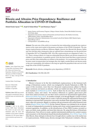
9. Risks 2021, 9, 74 9 of 13
In general, Ripple’s closing price has a significant impact on the closing prices of
Bitcoin and Binance when the pandemic is not considered in the model. However, the
closing price of Ripple has no impact on Bitcoin’s and Binance’s closing prices when the
pandemic is considered in the model. Similarly, in the long run, the closing price of Tron
has no impact on any of the cryptocurrencies’ closing price when the pandemic is not
considered in the model. However, it has a highly significant impact on the closing prices
of Bitcoin, Binance, and Ripple when the pandemic is considered in the model.
The impact of the COVID-19 pandemic on the closing prices of nine cryptocurrencies
in the short run is shown in Table 6. It is evident that the pandemic has a positive and
direct highly significant (at 1% level of significance) impact on the closing prices of Binance,
Ethereum, Stellar, and Tron and it has a mild (at 10% level of significance) impact on the
closing price of Ripple. The rest of the cryptocurrencies’ closing prices are not affected by
the COVID-19 pandemic.
Table 6. Impact of Pandemic (DP) in the Short Run.
D(BT) D(BC) D(BN) D(RP) D(EO) D(ET) D(LT) D(ST) D(TR)
0.005165 0.006750 0.022341 *** 0.012153 * 0.006938 0.015194 *** 0.007722 0.025631 *** 0.027721 ***
(0.00446) (0.00731) (0.00648) (0.00621) (0.00720) (0.00552) (0.00585) (0.00713) (0.00911)
*** and * represent the significance of coefficient at 1% and 10% level of significance respectively. In parenthesis are the standard errors.
To investigate the interrelationships among the cryptocurrencies in presence of the
COVID-19 pandemic, the variance decomposition of all the cryptocurrencies is depicted in
Figure 2. It is evident that the variation (almost 100%) in Bitcoin is due to itself and not
due to other cryptocurrencies. Furthermore, Bitcoin has a significant amount of portion
of the variation in all other cryptocurrencies like BitcoinCash, Binance and Eos (almost
40%), Ripple, Stellar, and Tron (around 20%). However, for these six cryptocurrencies, the
proportion of variation of Bitcoin is lesser than the cryptocurrency itself. Interestingly, for
Litecoin and Ethereum the proportion of Bitcoin (almost 50%) is greater than the proportion
of variation of cryptocurrency itself. All these results suggest that the variations in Bitcoin
are the sole stronger driver of the variations in all other eight cryptocurrencies. The results
of the variance decomposition when the COVID-19 pandemic is not considered are the
same, indicating again that in the long run, there is no significant impact of the COVID-19
pandemic on cryptocurrencies and hence they are resilient.

10. Risks 2021, 9, 74 10 of 13
portion of variation of Bitcoin is lesser than the cryptocurrency itself. Interestingly, for
Litecoin and Ethereum the proportion of Bitcoin (almost 50%) is greater than the propor-
tion of variation of cryptocurrency itself. All these results suggest that the variations in
Bitcoin are the sole stronger driver of the variations in all other eight cryptocurrencies.
The results of the variance decomposition when the COVID-19 pandemic is not consid-
ered are the same, indicating again that in the long run, there is no significant impact of
the COVID-19 pandemic on cryptocurrencies and hence they are resilient.
0
20
40
60
80
100
1 2 3 4 5 6 7
BT BC BN
RP EO ET
LT ST TR
Variance Decomposition of BT
0
20
40
60
80
100
1 2 3 4 5 6 7
BT BC BN
RP EO ET
LT ST TR
Variance Decomposition of BC
0
20
40
60
80
100
1 2 3 4 5 6 7
BT BC BN
RP EO ET
LT ST TR
Variance Decomposition of BN
0
20
40
60
80
100
1 2 3 4 5 6 7
BT BC BN
RP EO ET
LT ST TR
Variance Decomposition of RP
0
20
40
60
80
100
1 2 3 4 5 6 7
BT BC BN
RP EO ET
LT ST TR
Variance Decomposition of EO
0
20
40
60
80
100
1 2 3 4 5 6 7
BT BC BN
RP EO ET
LT ST TR
Variance Decomposition of ET
0
20
40
60
80
100
1 2 3 4 5 6 7
BT BC BN
RP EO ET
LT ST TR
Variance Decomposition of LT
0
20
40
60
80
100
1 2 3 4 5 6 7
BT BC BN
RP EO ET
LT ST TR
Variance Decomposition of ST
0
20
40
60
80
100
1 2 3 4 5 6 7
BT BC BN
RP EO ET
LT ST TR
Variance Decomposition of TR
Variance Decomposition using Cholesky (d.f. adjusted) Factors
Figure 2. Variance decomposition in presence of pandemic.
4. Conclusions
Due to the volatile structure of cryptocurrencies in the crypto stock-market, investors
and portfolio managers periodically demand shocks that can alter in degree across the
cryptocurrencies hinging on the co-movement of their price returns. Discoveries about
what causes volatility and directions of co-movements on the market by explicit factors
Figure 2. Variance decomposition in presence of pandemic.
4. Conclusions
Due to the volatile structure of cryptocurrencies in the crypto stock-market, investors
and portfolio managers periodically demand shocks that can alter in degree across the
cryptocurrencies hinging on the co-movement of their price returns. Discoveries about
what causes volatility and directions of co-movements on the market by explicit factors can
be difficult to measure from time to time owing to the precarious cyclic circumstances in the
entire system. In that point, our article analyzes the cointegration of top cryptocurrencies
based on daily prices on the crypto stock market by using the Johansen Cointegration
technique. The chosen cryptocurrencies are Bitcoin, Ethereum, Ripple, Litecoin, Eos,
BitcoinCash, Binance, Stellar, and Tron. Data sets are taken from coinmarketcap (2020) over
a period from 13 September 2017 to 21 September 2020. The result of this test demonstrates
that there is cointegration among the Bitcoin and other chosen altcoins in the market.

11. Risks 2021, 9, 74 11 of 13
Before conducting the Johansen test, we applied three different unit root tests to
determine the stationarity of the ten crypto currencies’ prices. Then, before going for the
Johansen cointegration test to test the existence of a long-run relationship among the ten
crypto price series, we checked for the appropriate lag length order. After choosing the
optimal lag order, finally, the Johansen cointegration test was carried out. In addition to
that, a vector error correction model (VECM) was estimated to investigate the long-run
cointegrating relationship as well as short-run relationships among the variables. The
results indicate that when the COVID-19 pandemic effect is not taken into account, Bitcoin
and Binance prices are not affected by the Ripple price. However, it is just the opposite
when the effect of the COVID-19 pandemic is considered. This implies that the pandemic
has a very grave impact on the inter-relationship of three crypto prices i.e., Bitcoin, Binance,
and Ripple. Similarly, when the pandemic is not accounted into the model then Tron
prices are not affecting any of the cryptocurrency prices. However, when the pandemic is
considered, then Tron affects the prices of Bitcoin, Binance, and Ripple.
Specifically, the magnitude of results reveals that some cryptocurrencies have a closer
relationship concerning their price dependencies as time goes by in the COVID-19 pan-
demic. It offers investors to allocate their portfolios to balance their risks in the pandemic.
Furthermore, even though each cryptocurrency has different narratives, aims, and func-
tions, there is no one winner on the stock market or our result does not demonstrate the
zero-sum game. There is a win-win situation among cryptocurrencies. Hence, policymak-
ers and regulators can take into account cryptocurrencies as potential alternative digital
assets to reduce the risks of their national assets for the crisis term and especially in crises
like the COVID-19 pandemic.
Our research provides objectively and reasonably adaptable analysis, especially for
beginner crypto enthusiasts and investors, who might take many needles risks or abide
by an over-cautious approach when they discover the crypto world from the scratch,
to minimize their risk and maximize their returns for the long-term. Since these top
cryptocurrencies in the stock market that we chose are safer and more stable due to their
long-established timeline in the pandemic. Hence, these top cryptocurrencies can be
accepted as the new asset opportunities because they have already proved their maturity
as compared to other assets.
Our results also touch upon that these top cryptocurrencies can be divided into subcat-
egories. Accordingly, when investors design their portfolio, they can make diversification
among these top cryptocurrencies to raise their money for the long-term. For instance,
Bitcoin, Ethereum, Ripple, and Litecoin are the cryptocurrencies that have the longest
history as compared to their counterparts. If we divide these four cryptocurrencies, making
an investment of those cryptocurrencies by matching with other altcoins among the top list
that we chose, it will offer investors a more diversified and balanced portfolio for the long
term. Furthermore, our analysis gives universal formula with a more global approach for
each investor from all over the world without regard to their nationality which means that
everyone holds the same risking portfolio. Cryptocurrencies, which are not controlled by
governments and national authorities, are not affected by government regulations, rather
they are affected by cyclical risks and volatility in the global financial system. To avoid
these risks, our results provide a narrowing analysis for the top cryptocurrencies from the
unlimited set of choices in crypto-asset allocation.
Overall, this article would be beneficial for investors who would like to diversify
their portfolios for the long term. Preparing a long-term portfolio would be more strategic
because of the “novel features of the market” as Shams (2019) defined in his paper. More
broadly, far from being static and narrow-minded, the market is ever-changing dynamically;
it permits investors, portfolio managers, and policymakers to design or manage their
portfolios by looking at them from different angles. The more they discover the operation
of business, politics, finance, and society as a whole, the more they have the capacity of
knowing what factors they should take into account to manage their wealth wisely. Finally,
when investors create investment strategies, focusing on altcoins together with Bitcoin can

12. Risks 2021, 9, 74 12 of 13
provide sustainability and resilience for the long term against the geopolitical risks due to
the tendency of the long-term relationship between Bitcoin and other altcoins even in the
tough periods of the COVID-19 pandemic.
Future studies can focus on other hourly, daily, and monthly prices of altcoins to inves-
tigate the long and short-term relationships among each other. For instance, researchers can
choose two different types of cryptocurrencies which each group has its strategy. Then, they
categorize them according to their purposes values, and narratives are given their white
papers. First, the cointegration relationship between each sub-group can be evaluated
within their group, and then researchers can compare the relationship of these two different
groups. Furthermore, the causality relationship of each cryptocurrency can be investigated
regardless of their group. Overall, results on the cointegration and causality relationship of
these different cryptocurrencies will shed light on the process of the cointegrated portfolio
for the investors in the financial market. Furthermore, it can also be investigated that
whether the COVID-19 pandemic has affected the main stock indices. A comparative
analysis of effect of COVID-19 on crypto market and the traditional stock market can be
carried out. In addition to this trading strategies likewise as proposed in (Brzeszczyński
and Ibrahim 2019) and (Batten et al. 2019) can be simulated about the interrelationship
among cryptocurrencies in presence of the COVID-19 pandemic.
Author Contributions: Conceptualization, A.F.A. and H.T.; methodology, A.U.I.K. and H.T.; soft-
ware, A.U.I.K. and H.T.; validation, A.F.A., A.U.I.K. and H.T.; formal analysis, A.U.I.K.; investigation,
A.F.A. and A.U.I.K.; resources, A.F.A. and A.U.I.K.; data curation, H.T.; writing—original draft prepa-
ration, A.U.I.K. and H.T.; writing—review and editing, A.F.A. and A.U.I.K.; visualization, A.F.A. and
A.U.I.K.; supervision, A.F.A. and A.U.I.K.; project administration, A.F.A.; funding acquisition, A.F.A.
All authors have read and agreed to the published version of the manuscript.
Funding: This research received no external funding.
Data Availability Statement: The data was obtained from https://coinmarketcap.com/ (accessed
on 3 November 2019). It is freely available.
Conflicts of Interest: The authors declare no conflict of interest.
References
Agosto, Arianna, and Alessia Cafferata. 2020. Financial Bubbles: A Study of Co-Explosivity in the Cryptocurrency Market. Risks 8: 34.
[CrossRef]
Nicaise, Nicolas, Hubert Anciaux, and Mikael Petitjean. 2019. Co-Movements in Market Quality of cryptocurrencies. Louvain: Louvain
School of Management.
Bação, Pedro, António Portugal Duarte, Helder Sebastião, and Srdjan Redzepagic. 2018. Information Transmission Between Cryptocur-
rencies: Does Bitcoin Rule the Cryptocurrency World? Scientific Annals of Economics and Busines 65: 97–117. [CrossRef]
Batten, Jonathan A., Janusz Brzeszczynski, Cetin Ciner, Marco CK Lau, Brian Lucey, and Larisa Yarovaya. 2019. Price and volatility
spillovers across the international steam coal market. Energy Economics 77: 119–38. [CrossRef]
Brooks, Chris. 2014. Introductory Econometrics for Finance, 3rd ed. Cambridge: Cambridge University Press.
Brzeszczyński, Janusz, and Boulis Maher Ibrahim. 2019. A stock market trading system based on foreign and domestic information.
Expert Systems with Applications 118: 381–99. [CrossRef]
Chuen, David LEE Kuo, Li Guo, and Yu Wang. 2017. Cryptocurrency: A new investment opportunity? The Journal of Alternative
Investments 20: 16–40. [CrossRef]
Ciaian, Pavel, and Miroslava Rajcaniova. 2018. Virtual relationships: Short- and long-run evidence from BitCoin and altcoin markets.
Journal of International Financial Markets, Institutions, and Money 52: 173–95. [CrossRef]
CoinMarketCap. 2019. Available online: https://coinmarketcap.com (accessed on September 23, 2020).
Dickey, David A., and Wayne A. Fuller. 1979. Distribution of the estimators for autoregressive time series with a unit root. Journal of the
American Statistical Association 74: 427–31.
Ethereum White Paper. 2019. Available online: https://ethereum.org (accessed on 3 November 2019).
Giudici, Paolo, and Paolo Pagnottoni. 2019. High Frequency Price Change Spillovers in Bitcoin Markets. Risks 7: 111. [CrossRef]
Joline, Göttfert. 2019. Cointegration among Cryptocurrencies: A Cointegration Analysis of Bitcoin, Bitcoin Cash, EOS, Ethereum,
Litecoin, and Ripple. Master’s Thesis, MA in Economics, University in Umeå, Umeå, Sweden.
Granger, Clive W. J., and Paul Newbold. 1974. Spurious regressions in econometrics. Journal of Econometrics 2: 111–20. [CrossRef]
Harris, Richard, and Robert Sollis. 2003. Applied Time Series Modelling and Forecasting. New York: Wiley.

13. Risks 2021, 9, 74 13 of 13
Huang, Yingying, Kun Duan, and Tapas Mishra. 2021. Is Bitcoin really more than a diversifier? A pre- and post-COVID-19 analysis.
Finance Research Letters 2021: 102016. [CrossRef]
J McNeil, Alexander. 2021. Modelling Volatile Time Series with V-Transforms and Copulas. Risks 9: 14. [CrossRef]
Johansen, Søren. 1995. Likelihood-Based Inference in Cointegrated Vector Autoregressive Models. Oxford: Oxford University Press on
Demand.
Johansen, Soren, and Katarina Juselius. 1990. Maximum likelihood estimation and inference on cointegration—With applications to
the demand for money. Oxford Bulletin of Economics and Statistics 52: 169–210. [CrossRef]
Kwiatkowski, Denis, Peter CB Phillips, Peter Schmidt, and Yongcheol Shin. 1992a. Testing the null hypothesis of stationarity against
the alternative of a unit root: How sure are we that economic time series have a unit root? Journal of Econometrics 54: 159–78.
[CrossRef]
Kwiatkowski, Denis, Peter CB Phillips, Peter Schmidt, and Yongcheol Shin. 1992b. Testing the null hypothesis of stationarity against
the alternative of a unit root. Journal of Econometrics 54: 159–78. [CrossRef]
Leung, Tim, and Hung Nguyen. 2019. Constructing cointegrated cryptocurrency portfolios for statistical arbitrage. Studies in Economics
and Finance 36: 581–59. [CrossRef]
Mariana, Christy Dwita, Irwan Adi Ekaputra, and Zaäfri Ananto Husodo. 2021. Are Bitcoin and Ethereum safe-havens for stocks
during the COVID-19 pandemic? Finance Research Letters 38: 101798. [CrossRef]
Phillips, Peter CB, and Pierre Perron. 1988. Testing for a unit root in time series regression. Biometrika 75: 335–46. [CrossRef]
Resta, Marina, Paolo Pagnottoni, and Maria Elena De Giuli. 2020. Technical Analysis on the Bitcoin Market: Trading Opportunities or
Investors’ Pitfall? Risks 8: 44. [CrossRef]
Ripple White Paper. 2019. Available online: https://ripple.com (accessed on 3 November 2019).
Shams, Amin. 2019. What Drives the Covariation of Cryptocurrencies Returns? Paper presented at the Association of Financial
Economists American Economic Association Beyond Bitcoin Paper Session Conference, Atlanta, GA, USA, January 4–6.
Sovbetov, Yhlas. 2018. Factors Influencing Cryptocurrency Prices: Evidence from Bitcoin, Ethereum, Dash, Litcoin, and Monero.
Journal of Economics and Financial Analysis 2: 1–27.
Tron White Paper. 2019. Available online: https://tron.network (accessed on 3 November 2019).
Umar, Muhammad, Chi-Wei Su, Syed Kumail Abbas Rizvi, and Xue-Feng Shao. 2021. Bitcoin: A safe haven asset and a winner amid
political and economic uncertainties in the US? Technological Forecasting and Social Change 167: 120680. [CrossRef]
Zhang, Hongwei, and Peijin Wang. 2021. Does Bitcoin or gold react to financial stress alike? Evidence from the US and China.
International Review of Economics Finance 71: 629–48.